Abstract
With the aim of simultaneously improving fishery production and utilizing forestry and oyster fishery wastes, three types of artificial timber reefs (ATRs)—constructed from simple timbers, timbers with oyster shells from local oyster farms, and timbers with leaves/branches from forest thinning—were deployed in Mitsu Bay, Japan. We developed a food web model to investigate the relative efficacies of these ATR types compared with the bare, sandy seafloor. The model described the material flow through the food webs formed in each ATR type and their potential to increase fisheries production. The model outputs were validated with observational data over three years. The model fit the observed biomass of both prey animals and fish predators. The simulation results highlighted that ATRs, particularly those with additional materials, had two to three times higher feeding flow than the sandy seafloor and resulted in increased fish biomass. Fish catch doubled in the ATR areas compared to the bare seafloor. Aside from providing a feeding ground, the complexity of the ATRs with additional materials likely acts to provide shelter for juvenile fish. ATR deployment using by-products such as those mentioned above may not only enhance fish stock but also help foster the establishment of a recycling-oriented society.
1. Introduction
Artificial reefs (ARs) are human-made structures deployed in the aquatic ecosystem for various services and benefits. The deployment of ARs is believed to benefit fishery yield by providing a habitat for fish and their feeds [1,2]. The type of structures and materials used for the construction of ARs is key for meeting the expected goals. The materials used for AR construction vary around the world, ranging from either natural materials such as rocks, shells, and wood or artificial materials such as concrete, fiberglass, tires, vessels, and vehicles [3].
In Japan, fishery production has been decreasing over the past few decades [4]. The current estimated domestic fishery production is approximately 60% and the remaining 40% is imported. Ensuring the long-term sustainability of fisheries is essential to reduce dependency on imported seafoods. The national government attempted to increase fish stocks by deploying ARs in the coastal waters [5]. During the 1950s, with considerable government funding, ARs were primarily constructed of concrete [6]. Recently, with less funding from the central government, the trend of AR material has shifted from concrete to natural materials such as timber. The government of Higashi-Hiroshima City, in coordination with the local fishery association, deployed artificial timber reefs (ATRs) in Mitsu Bay, Japan in late 2015. Timber is plentiful, as a by-product of forest thinning in the forested areas surrounding this city. It is also reported that timbers attract fish more efficiently than other materials, and hence, they are ideal as an AR construction material [7]. In Mitsu Bay, the main fishery activity is oyster cultivation. This industry generates large quantities of oyster shells. Thus, we tested oyster shells as supplementary materials for ATRs, as well as the leaves and branches of timbers from thinning.
The use of timbers for ARs is not uncommon in Japan [8] and elsewhere [9,10,11]. Nevertheless, there have been few numerical studies in terms of the efficacy of ARs in structuring food webs in new ecosystems and their implications in increasing fishery production [12,13]. The dynamics of predator–prey interactions within the food web structure of an aquatic ecosystem are multifactorial and thus highly complex. ATR structures provide settlement locations for sessile organisms on the reefs and for benthic organisms beneath the reefs. Further, ATRs may enhance the production of higher trophic level animals such as fish through changes in prey composition, resulting in the formation of a new ecosystem [14,15].
In the present study, we focused on the difference in efficacy of the three types of ATRs—simple timbers, timbers with oyster shells, and timbers with leaves/branches. The efficacies, in terms of food web structure, were tested by applying a numerical model. Thus, the objectives of the study were as follows: (1) to evaluate the increase in fish production as a result of the presence of ATRs, particularly with the supplementary materials such as oyster shells and leaves/branches, and (2) to understand the difference in material flows induced by the different animal and fish compositions created in the three different types of ATRs by numerical model analyses.
2. Materials and Methods
2.1. Artificial Timber Reefs and Their Deployment
ATRs (1.5 m × 1.5 m × 1.5 m) were constructed with Japanese cypress timbers in a cube-shaped parallel cross, following the method of Alam et al. [1] (Figure S1). A total of 15 ATRs (three simple timber reefs; six timber reefs with oyster shells, ATRsOS; and six timber reefs with leaves and branches, ATRsLB) were deployed in November 2015 at 10 m depth and arranged as shown in Figure 1 at each of two locations in Mitsu Bay, Higashi Hiroshima: Kazahaya (34°17′28.8″ N, 132°48′26.4″ E) and Kidani (34°17′39.8″ N, 132°50′21.8″ E). Bare, flat, sandy seafloor areas 10 m from the edge of the ATRs at Kazahaya and 20 m from the ATRs at Kidani were used to compare the enhancement of fish production as a result of ATRs.
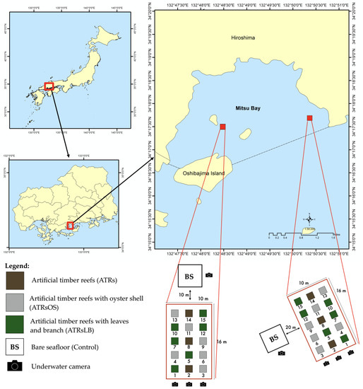
Figure 1.
Experimental design and the locations of artificial timber reefs deployed in Mitsu Bay, Hiroshima Prefecture, Japan.
2.2. Sampling
Field observations were conducted eight times for three years after ATR deployment: January and July 2016; January, July, and November 2017; and January, March, and August 2018. Prey (zooplankton, attached and benthic) organisms were sampled from the ATRs and bare seafloor. In the ATR deployment area, zooplankton samples were collected using a 100-μm mesh Kitahara plankton net, 22.5 cm in diameter (0.04 m−2), vertically towed from the bottom to the surface just beside the ATR constructions. The zooplankton samples were fixed with 5% formaldehyde in the final concentration; then, they were sorted, counted, and weighed in the laboratory. Test pieces of timber and net baskets containing supplementary materials were collected by two SCUBA divers. All samples of test pieces of timber and the net basket were packed in plastic bags to prevent the organisms on and in them from escaping. Benthic organisms were also collected from the top 5 cm of sediment at the edge of each ATR using a 25 cm × 25 cm (625 cm2) grab sampler. All samples were sieved with a 1.0-mm mesh, fixed in 10% formaldehyde, and transported to the laboratory for sorting, counting, and weighing.
Fish abundance was evaluated using video recordings. This method was adopted as it provides permanent recordings of data, permits observations for fixed time periods, and enables data collection under conditions unsafe for diver-based assessments [16,17]. Furthermore, video recording avoids miscalculations that can occur when diver movements cause fish escape reactions, resulting in the loss of fish to observation. Neither method works at night, so nocturnal fish biomass was underestimated. In total, eight underwater cameras (Hero Session 4, GoPro Co. Ltd., San Mateo, CA, USA) were placed 1.5 m in front of each ATR and bare seafloor, i.e., one camera each for the different types of ATRs and the bare seafloor in the two sites. Each camera had a field of view covering the associated single ATR structure plus 1 m to each side. The total volume observed by each camera was estimated to be 11.67 m3. Camera recordings were operated for a net of one hour during 9:00–11:00 in the morning. With this way of sampling, we missed nocturnal fish. However, the operation of the camera at night would have required additional light to catch fish in video recording, which may have affected the results, particularly by selecting fish with positive phototaxis; as such, it was decided that nocturnal fish would not be observed, and the recording would only be done during daytime. All of the fish observed in the footage were classified to the species or genus level and enumerated. The fish abundance determined in the present study resembled the fish abundance (MaxN) metric of Scott et al. [18]. Fish abundance is the maximum number of fish species observed in a single frame of footage during one deployment [19]. As fish size measurements based on the video scenes were inaccurate, size ranges (0–15 cm, 15–30 cm, and >30 cm) were applied, and the biomass was estimated using the published length–weight relationship for each fish species [20]. The averages of the prey and predator biomasses from the two sites for each treatment were then used for further analysis in the model.
In addition to the samplings of biotic parameters, abiotic parameters that affect the growth of primary producers were measured. Chlorophyll-turbid meters (INFINITY-CLW, JFE Advantech, Co. Ltd., Kobe, Japan) were used to record temperature, relative chlorophyll fluorescence, and turbidity, and PAR loggers (DEFI2-L, JFE Advantec, Co. Ltd., Kobe, Japan) were used to record the underwater photon density; the chlorophyll-turbid meters and photosynthetic active radiation (PAR) loggers were attached on the ATR structures at each site and regularly replaced at every sampling event. The sampling interval was set to every hour, and the sample number was 10 at each sampling event. We averaged the 10 data points in each hour for use.
2.3. Structure of the Numerical Model
The numerical model developed in this study described the food webs created in the ATRs and differences in the material flow seen in the different types of ATRs. In each case, simplified frameworks were composed that illustrated the dynamics of the predator–prey relationships (Figure 2). Each ATR had 21 compartments and each bare seafloor had 8 compartments, reflecting its scarcity of residing organisms as a result of not having ATR structures. In all 21 compartments in the ATRs, biomass changes over time were governed by biotic processes and by each compartment’s relationship with the other compartments, as shown in Table 1.
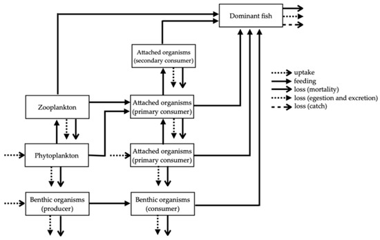
Figure 2.
Simplified framework for predator–prey relationships in artificial timber reefs and bare seafloor areas.

Table 1.
Mass balance equations for the compartments used in the present numerical model.
Changes in the biomass of the primary producers, planktonic microalgae (MIA), benthic microalgae (MIAb), and macroalgae (MAA) were functions of nutrient uptake, temperature, and light intensity. Their loss processes were excretion, temperature-dependent mortality, and grazing by herbivores. The changes in the biomasses of zooplanktons, attached animals residing in the ATRs, and benthic animals were functions of food availability, competition with other animals at the same trophic level, egestion, mortality, and predation.
For the changes in fish biomass, swimming behavior was taken into consideration as described below, along with physiological functions such as grazing, excretion, and mortality applied as described above. Unlike attached and benthic organisms, which are mostly sessile, some fish are mobile and swim in and around the observation area. The change in fish biomass was affected by fish mobilization in addition to the changes governed by feeding, egestion, excretion, natural death, and catch described by Equation (1) [20].
where N is the fish abundance (inds m−3) and W is the individual wet weight (g ind−1) estimated from the length (TL) and weight (BW) relationship of each fish species in Equations (2)–(7) [21].
dfish/dt = N × dW/dt + W × dN/dt
BSE BW = 2.818 × 10⁻² TL2.98
BRO BW = 1.318 × 10⁻² TL3.06
JSU BW = 1.148 × 10⁻² TL2.95
MRA BW = 1.175 × 10⁻² TL3.12
BSC BW = 2.188 × 10⁻² TL2.91
RSE BW = 1.413 × 10⁻² TL3.00
The dominant fish species incorporated into the present model were previously categorized as resident fish [22,23]. These fish tended to remain in the AR area. Other species were designated as visitor fish and were observed only once in the AR area. Transient fish such as Japanese mackerel Trachaurus japonicus were observed infrequently and would have contributed a disproportionate amount to the total biomass. Hence, they were excluded from the model calculation to avoid introducing bias into the analysis of the AR ecology. Eliminating the influences of visitor and transient fish from the analysis reveal more pronounced seasonal variations in fish abundance and biomass [24].
The feeding preference of each fish was also incorporated in the model. The values used in this model lie within the ranges reported in published papers (Table 2). Fish egestion and excretion were set at the same values for all fish, at 20% and 11% of feeding, respectively [25,26]. When the fish reached minimum catch size, loss to fish catch became an exit flow from the relevant biomass compartment, with the rate depending on the catch. The catch size of each fish was determined from information available from the internet, fishermen, and market sources. The daily catch rates were adjusted so that the temporal changes in fish biomass fit the observed values, and also to obtain minimum percent bias (PBIAS).
Table 2.
Summary of feeding habits of dominant fish species observed in Mitsu Bay, which were incorporated in the model.
The equations used in all the processes are as described below. The uptake of algae (e.g., MIA) is as expressed in Equation (8), dependent on temperature and light intensity.
uptake (MIA) = µmax (MIA) × exp (kT × T) × I/Iopt exp(1 − (I/Iopt)) × (MIA)
The function of growth of attached, benthic organisms and fish (e.g., SHR) is shown in Equation (9). Furthermore, the function of excretion, egestion, and mortality for organisms are shown in Equations (10)–(12). These equations are also applied to the other organisms in this study.
growth (SHR) = μ(SHR) × eat (SHR) × (SHR)
exc (SHR) = kexc (SHR) × eat (SHR)
fae (SHR) = kf (SHR) × eat (SHR)
mortal (SHR) = kmor (SHR) × growth (SHR)
For fish, an addition function of catch (e.g., BSE) was used, as shown in Equation (13).
catch (BSE) = IF TL ≥ minimum catch size THEN kcat (BSE) × (BSE) ELSE 0
The parameters used in this study are shown in Table 3. Although most of the model parameter values were obtained from published literature, some of them were tuned to fit the model output to the observed data. The numerical model was developed using STELLA Architect for Macintosh (v. 1.6.0) and run with a time step of 0.015 day. Calculations were conducted for 1020 days by a 4th-order Runge–Kutta method.
Table 3.
List of parameters used in the model.
2.4. Statistical Analysis
The data obtained from the observations from the two sites were compared to investigate the efficacy of the different types of ATRs in terms of increase in prey animals and fish. The difference in attached and benthic organisms and fish were tested using one-way ANOVA after verifying the homogeneity of variances. The average values of the two sites, along with their variations, were used to validate the model, and checked with the percent bias (PBIAS), which is a measure of over- and under-estimation of bias for predicted values from the measured values, and it is expressed as a percentage [33]. The performance rating of the model outputs was judged using the criterion as follows: very good (PBIAS < ±25%), good (±25 PBIAS < ±40), satisfactory (±40 PBIAS < ±70), and non-satisfactory (≥±70) [34].
3. Results
Organisms began to encrust on the ATR surfaces soon after ATR deployment. The calculations from the numerical model of the attached and benthic animal biomass showed good and satisfactory fits to all observed values; the PBIAS values were in the 25–70% range for all, except for bivalves (BIV), errant worm (EWO), caprellid (CAP), and other amphipods (OAM) in the artificial timber reefs with leaves and branches (ATRsLB) (Table S1). The biomass values for all attached organisms in the artificial timber reefs with oyster shells (ATRsOS) and ATRsLB were higher than those for the simple ATRs (Figure 3). CAP, SHR, BIV, EWO, and SWO were significantly higher in ATRsOS and ATRsLB compared to ATRs (p < 0.05) (Table 4). Among the benthic organisms, the biomass values for two major groups, benthic bivalves (BIVb) and sedentary worms (SWOb), did not differ significantly between the ATRs and the bare seafloor areas during early deployment, although biomass in the ATRs was slightly higher in the third year (Figure 4).
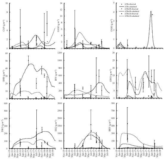
Figure 3.
Relative temporal changes in attached organisms on simple artificial timber reefs and those with either supplementary oyster shells or supplementary leaf and branch materials.
Table 4.
The average observed biomass of prey and fish in artificial timber reefs (ATRs) and bare seafloor. One-way ANOVA was applied to check if there were statistical differences between the groups. ATRsOS: artificial timber reefs with oyster shells, ATRsLB: artificial timber reefs with leaves and branches.
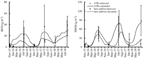
Figure 4.
Relative temporal changes in benthic organisms in artificial timber reefs and bare seafloor areas.
The annual average stocks and flows within the food webs in the three ATRs and bare seafloor areas are shown in Figures S2–S5. The main inputs for attached organisms were feeding on producers: phytoplankton (PHY) in the water column, and microalgae (MIA) and macroalgae (MAA) on the timber surfaces. Zooplankton (ZOO) and other organisms such as gammarids (GAM), caprellids (CAP), and other amphipods (OAM) were eaten by shrimp (SHR) and errant worms (EWO). In the sediment, the main input for BIVb and SWOb growth was feeding on benthic microalgae (MIAb) and PHY. There was a larger feeding flow from producers in ATRsOS and ATRsLB than was seen in simple ATRs. The total grazing rates on algae (PHY, MIA, MAA, and MIAb) by attached organisms and benthic animals were an order of magnitude larger in ATRsOS and ATRsLB reefs (69.2 and 49.7 g m−3 day−1, respectively) than that in simple ATRs (4.3 g m−3 day−1). At the bare seafloor, the rate was also low, with a value of 2.8 g m−3 day−1 (Figures S2–S5).
Animals, regardless of whether attached or benthic, were the prey of fish, varying substantially, as summarized in Table 2. GAM, CAP, OAM, and SHR were generally eaten by most of the dominant fish, so their biomass profiles were shaped by heavy predation (Table 2). SWO was less eaten by dominant fish or could escape from predation, and consequently it had higher biomass values, especially in ATRsOS and ATRsLB. Their biomass was shaped mainly by the losses on egestion and natural mortality. Bryozoan (BRY) and sea squirt (SSQ) were also not fed on by fish as much, and their biomass profile was shaped by natural mortality. In the first year of the ATRs deployment, the BRY biomass was highest on the simple ATRs and ATRsLB reefs, and it was second highest on the ATRsOS reefs (Figure 3). However, it steadily decreased from the second year onwards, while SSQ biomass increased.
Twenty-nine fish species were observed at the study sites during the three years of field observations. Six species were found most frequently and were targeted for calculation in the model as dominant fish. Black rockfish Sebastes inermis (BRO) and Japanese surfperch Ditrema temmincki (JSU) were highly associated with all ATRs at all sampling dates. There were no clear associations of these fish species with the bare seafloor, as the fish only roamed over them.
The model reproduced the observed fish biomass (Figure 5). The PBIAS values showed very good, good, and satisfactory fits to all observed values, i.e., the PBIAS values were in the 25–70% range (Table S1), except for black scraper Thamnaconus modestus (BSC), which was categorized as non-satisfactory. However, the trend of the calculated value followed the observed data except at the point in the third year of deployment where there was a large gap between the observed and calculated values. The average observed black seabream Acanthopagrus schlegelii (BSE) biomass was 62, 31, 59, and 48 g m−3 in ATRs, ATRsOS, ATRsLB, and bare seafloor, respectively. While the BSE observed around ATRs were mainly juveniles of smaller size, as recorded in the video, those observed in bare seafloor areas were mostly adult size. The highest average BRO biomass was recorded around the ATRsLB (223 g m−3), followed by that around the simple ATRs (173 g m−3) and that around the ATRsOS (140 g m−3). Meanwhile, no BRO was observed in bare seafloor sites at any time during the observation period. The BRO biomass increased over time in all ATRs, peaking during the colder season and troughing during the warmer season.
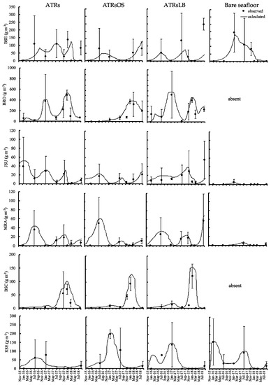
Figure 5.
Numerical model simulation outputs (connected curves) and observed values (average: filled dot; bar: deviation) for fish biomass at the different types of ATRs and bare seafloor in Mitsu Bay, Japan.
The JSU biomass was highest in the colder season and lowest in the warmer season. The average JSU biomass were 14, 8, and 17 g m−3 in ATRs, ATRsOS, and ATRsLB, respectively. In contrast, the average JSU biomass in bare seafloor areas was only 0.5 g m−3. The average multicolorfin rainbowfish Parajulis poecilopterus (MRA) biomass was relatively equal across all ATRs and was highest in the warmer season and lowest in the colder season. The average MRA biomass for the ATRs and ATRsOS was 9 g m−3 in each case. This was somewhat lower than the average MRA biomass values for the ATRsLB, which was 15 g m−3. The average MRA biomass in bare seafloor areas was only 0.9 g m−3. For all ATRs, the average BSC biomass had increased by summer 2017, two years after deployment. The average BSC biomass values was fairly similar among ATRs, whereas in bare seafloor areas, no BSC were observed. The average red seabream Pagrus major (RSE) biomass were 19, 45, and 29 g m−3 in ATRS, ATRsOS, and ATRsLB, respectively. In the bare seafloor areas, it was 55 g m−3.
The model calculation of total consumption of attached and benthic animals by fish was highest in the ATRsLB, at a rate of 37.9 g m−3 day−1, followed by the simple ATRs and ATRsOS, at 27.6 g m−3 day−1 and 27.5 g m−3 day−1, respectively, while in the bare seafloor areas, it was only 12.5 g m−3 day−1. About 10% of outflow losses from fish stocks were due to excretion in both ATR and bare seafloor areas; a further 22–24% and 20% were due to egestion in the ATRs and bare seafloor areas, respectively. The natural mortality of attached and benthic animals constituted 25–28% of the loss in the ATRs and 17% in bare seafloor areas.
The calculated fish catch made further reductions to these natural losses. Its impact differed among ATRs. The loss values were approximately 3.7 kg m−3 year−1, 4.2 kg m−3 year−1, 5.4 kg m−3 year−1, and 2.3 kg m−3 year−1 in the simple ATRs, ATRsOS reefs, ATRsLB reefs, and bare seafloor areas, respectively. BRO was the most frequently caught fish in all of the ATRs, at 50%, 33%, and 51% in the simple ATRs, ATRsOS, and ATRsLB, respectively. In bare seafloor areas, the fish catch accounted for 52% of total fish loss, and the most frequently caught fish there was RSE (90%).
4. Discussion
Novel community assemblies developed rapidly (within three months) following the deployment of the ATRs, with the attachment of organisms to the ATR structures. ATRs also supply prey for higher trophic level animals by enabling prey animals to reside inside the construction materials. Japanese cypress trees, the timbers from which were used for the ATR frameworks in this study, emit volatile phytoncides that protect the trees from wood-boring invertebrates. For this reason, this tree has superior durability and is commonly used as a construction material in traditional Japanese buildings [74,75]. However, this repellent effect is relatively weak in seawater, as reported by Masuda et al. [7]. Nevertheless, the rough surface of the cypress wood supports organism attachment and growth. This is an advantage of using timbers, unlike the concrete materials that are commonly used for ARs around Japan.
The relatively higher prey biomass on the modified ATRs (ATRsOS and ATRsLB) was observed comparing to that on the simple ATRs. This suggests that the complex structures formed inside the ATRs with the supplemental materials may have contributed to the increase in the number of organisms attached in the space. The simulation results reproduced the higher attached animal biomass in ATRsOS and ATRsLB compared to the simple ATRs. To some extent, this can be attributed to the dominant presence of filter feeders on the additional settlement materials. This domination of filter feeders in the biomass has also been commonly reported in other studies, as in epibiotic communities in the ARs in Hong Kong [76] and in the designated artificial reef (DAR) off the coast of Sydney [77].
After the deployment of ATRs, the first settler was bryozoan as represented on ATRsLB. Bryozoans are reported to be the pioneer species in the newly formed ecosystem of this type [78]. Bryozoan biomass was succeeded by sea squirt in the second year, which was possibly because of space exclusion and food source competition. A succession from bryozoan to sea squirt on wood panels was also observed in Hong Kong waters [79]. Sea squirt is often observed as an invasive species in marine structures [80]. It may penetrate mature assemblages and subsequently become the dominant species [81,82]. Bryozoans and sea squirt are not likely the animals fed preferentially by fish. However, these filter feeders may act to collect particulate organic matter including phytoplankton and supply organic matter to the benthic animals [83,84].
Bivalve and sedentary worm biomass increased over time against the early occupation by bryozoans and sea squirt. Bivalves and sedentary worms are qualified food for fish [85]. Our study emphasizes the importance of ATR structures in that they may contribute to increasing levels of prey animals for fish. The attached and benthic prey organisms on all ATRs seemed to support far more fish biomass than in bare seafloor areas, creating and shaping new food webs. AR deployment in the Caribbean significantly altered the faunal biomass [86]. Thus, ATR deployment exerts an impact by activating secondary production and further energy transfer to higher trophic levels. As seen in Figures S2–S5, secondary production and energy transfer were higher in all ARs than that in the bare seafloor areas. In the benthic system, feeding flow to benthic bivalves and benthic sedentary worm in the ATRs was almost the same as that in bare seafloor areas at the beginning, as they were located in what could be, in principle, considered a fairly homogenous environment at their spatial scale. Nevertheless, slightly larger flow was simulated in the ATRs in the following years, when biomass in the ATRs was higher than in the bare seafloor areas.
Overall, organism biomass on the ATRsLB initially increased, but one year after post-deployment, it declined as the structure decayed. Photographs taken by divers confirmed that the leaves and branches had undergone degradation within approximately 18 months (Figure S6). Such loss of epifaunal communities after the decay of substrate materials was also reported elsewhere [85,87]. In contrast, the ATRsOS were able to maintain their shape and the biomass of the organisms attached on them, although the fish biomass was slightly lower than that of the ATRsLB. Although the major occupants in fish species were the same consisting of black rockfish and Japanese surfperch in all ATRs, the size of them were small in the ATRsOS and ATRsLB compared to that in the simple ATRs. It is said that the number of living spaces in ARs has a positive correlation to fish production [88]. Our ATRs consisted of timber logs stacked in parallel cross formation and furnished to provide shelters for juvenile fish. Thus, ATRsOS and ATRsLB, with their additional materials, are more likely to encourage the proliferation of smaller fish due to the many small, interstitial spaces provided [89], and these refuge sites promote the aggregation of smaller fish in ARs [90].
Wintertime increases in feeding pressure due to the increase of fish biomass may have depleted the prey animal biomass, causing the observed low animal biomass in this compartment during winter. The model corroborated the observations in terms of the seasonal variations in the dominant fish species at all of the ATRs and bare seafloor areas. Both black rockfish and black scraper increased in numbers in winter and contributed to the decrease in prey animal biomass in all ATRs. The increase in feeding pressure by black seabream and multicolor rainbowfish resulted in the loss of shrimp and other amphipods in the simple ATRs, gammarid, bivalves, and other amphipods in the ATRsOS, and gammarid and other amphipods in the ATRsLB (Figure 3).
The dominant fish incorporated into the model were commercial species that are commonly captured by local fishermen in Mitsu Bay. The estimated annual fish catch in the ATR areas (4.4 kg m−3 year−1) was twice as high as compared to that in the bare seafloor areas (2.3 kg m−3 year−1). Our calculation was lower than those of large ARs (16 kg m−3 year−1) and regular-size ARs with 1–2-m−3 chamber modules (20 kg m−3 year−1) reported in previous studies [91,92]. The relatively low estimation in the present study may be explained by the short observation period after the settlement (the ecosystem has not matured) and other several reasons such as the omission of transient fish from the calculations and oligotrophic conditions in the bay.
The results of the present study indicated that the ATRs deployed in Mitsu Bay promoted the creation of food webs that established a much greater availability of prey organisms for a wide range of commercially important fish species. This finding was confirmed by the output of a numerical model using predator–prey relationship inputs. The ATR structure serves various purposes as a new habitat, especially for those with additional materials where the diversity indices of attached organisms were higher than those in the simple ATRs [1]. This indicates that leaves and branches create extra space, which could work as shelter for juvenile fish. Oyster shells function in the same manner but last much longer than leaves and branches. Oyster shells are by-products of local aquaculture. Their use, along with timber from forest thinning, for ATR construction is a good way to encourage a recycling-oriented society, especially in Japan, which has large forests and relatively low fishery production.
In our study, only 30 ATRs were deployed, which are not likely to increase fish stock dramatically in the bay. In practice, it will be necessary to increase the number of ATRs in order to achieve fish stock recovery [93]. This requires further calculation (i.e., sensitivity analysis) on how many ATRs will be needed to improve fisheries production significantly in the deployment area. A regular repeated deployment of ATRs will be needed because of the short lifespan of the materials. In our regular observations conducted 48 months after the deployments, some of the frames forming the ATR were broken down, as shown in Figure S7. As natural products, the decomposed timbers may act as a source of organic matter, which would work positively in the aspect of material cycling in oligotrophic waters as in Mitsu Bay. Increasing the area of ATR deployment may help increase fishery production in Mitsu Bay. This idea can be applicable to the whole Seto Inland Sea area where the fishery production has been decreasing because of oligotrophication [94]. As we mentioned in an earlier paragraph, the usage of coastal areas is strictly controlled by the central and local government in addition to fishermen’s unions. It would be difficult to change the social system in a short amount of time. The fisheries law, which is the basic law describing the rules of fisheries in Japan, is planned to be revised in December 2020. Under the new law, considering the decrease in the number of fishermen, non-profit organizations (NPOs), non-governmental organizations (NGOs), and private companies will be allowed to join fishery activities under the condition of conserving the fisheries environments. At this stage, we will require proposals based on scientific knowledge, as in the present study, in collaboration with all involved sectors such as fishermen, forest keepers, local government, NPOs, NGOs, and volunteers, to increase fishery production while maintaining environmental conditions.
Supplementary Materials
The following are available online at https://www.mdpi.com/2073-4441/12/7/2013/s1, Figure S1: Artificial timber reefs (ATRs) used in the present study. (a) The appearance before deployment in Mitsu Bay, (b) at 1 month later, and (c) at 25 months later after deployment in the seawater. The net basket placed in the middle of frame was filled with additional material, oyster shells or leaves and branches. Table S1: Results of PBIAS calculated for the deviations of the calculation outputs from the observed values for each attached, benthic organism and fish. Figure S2: Annual average biomass stock (g m−3) (box) and flow (g m−3 d−1) (arrow) on simple artificial timber reefs for three years of 2016–2018. Abbreviations of stocks are same as those in Table 1. Figure S3: Annual average biomass stock (g m−3) (box) and flow (g m−3 d−1) (arrow) on artificial timber reefs with supplementary oyster shell material for three years of 2016–2018. Abbreviations of stocks are same as those in Table 1. Figure S4: Annual average biomass stock (g m−3) (box) and flow (g m−3 d−1) (arrow) on artificial timber reefs with supplementary leaf and branch material for three years of 2016–2018. Abbreviations of stocks are same as those in Table 1. Figure S5: Annual average biomass stock (g m−3) (box) and flow (g m−3 d−1) (arrow) in bare seafloor areas for three years of 2016–2018. Abbreviations of stocks are same as those in Table 1. Figure S6: Decayed supplemented leaves and branches packed in a net basket after one and a half years of deployment. Figure S7: The condition of ATR that was broken down after 48 months of deployment.
Author Contributions
Conceptualization, J.F.A. and T.Y.; methodology, J.F.A., T.Y. and T.U.; validation, J.F.A.; formal analysis, J.F.A.; investigation, S.N. and K.H.; data curation, T.U., S.N. and K.H.; writing—original draft preparation, J.F.A.; writing—review and editing, T.Y.; supervision, T.Y. and T.U.; project administration, T.Y.; funding acquisition, S.N. and K.H. All authors have read and agreed to the published version of the manuscript.
Funding
This research was funded by the Cabinet Office, Government of Japan, through its Regional Revitalization and Local Residents Life, Emergency Assistance Grant (Local Creation Proactive) 2015 program and the Program for Investigation of Fish Species Gathering on Artificial Timber Reefs for 2016–2018 by Higashi-Hiroshima City. Jamaluddin Fitrah Alam was supported by Lembaga Pengelola Dana Penelitian (Indonesia Endowment Fund for Education) (LPDP) Doctoral Degree Scholarship [contract no. PRJ-3186/LPDP.3/2016].
Acknowledgments
We thank Wahyudin P. Sasmita and the Kuzira Diving Center crew for their assistance with field sampling.
Conflicts of Interest
The authors declare no conflict of interest.
References
- Alam, J.F.; Yamamoto, T.; Umino, T.; Nakahara, S.; Hiraoka, K. Diversity of attached marine life in different types of artificial timber reefs. IOP Conf. Ser. Earth Environ. Sci. 2019, 370, 012034. [Google Scholar] [CrossRef]
- Xu, Q.; Zhang, L.; Zhang, T.; Zhou, Y.; Xia, S.; Liu, H.; Yang, H. Effects of an artificial oyster shell reef on macrobenthic communities in Rongcheng Bay, East China. Chin. J. Oceanol. Limnol. 2014, 32, 99–110. [Google Scholar] [CrossRef]
- Baine, M. Artificial reefs: A review of their design, application, management and performance. Ocean Coast. Manag. 2001, 44, 241–259. [Google Scholar] [CrossRef]
- Statistic Bureau. Ministry of Internal Affairs and Communications Stastistical Handbook of Japan 2017. Available online: https://www.stat.go.jp/english/data/handbook/pdf/2017all.pdf (accessed on 20 April 2019).
- Ministry of Agriculture Forestry and Fisheries. Trend in Fisheries 2014. Available online: https://www.maff.go.jp/e/data/publish/attach/pdf/index-79.pdf (accessed on 20 April 2019).
- Thierry, J.M. Artificial reefs in japan—A general outline. Aquac. Eng. 1988, 7, 321–348. [Google Scholar] [CrossRef]
- Masuda, R.; Shiba, M.; Yamashita, Y.; Ueno, M.; Kai, Y.; Nakanishi, A.; Torikoshi, M.; Tanaka, M. Fish assemblages associated with three types of artificial reefs: Density of assemblages and possible impacts on adjacent fish abundance. Fish. Bull. 2010, 108, 162–173. [Google Scholar]
- Ito, Y. Artificial reefs function in fishing grounds off Japan. In Artificial Reefs in Fisheries Management; CRC Press: Boca Raton, FL, USA, 2011; pp. 239–264. [Google Scholar]
- Relini, G.; Relini, L.O. Artificial reefs in the ligurian sea (northwestern mediterranean): Aims and results. Bull. Mar. Sci. 1989, 44, 743–751. [Google Scholar]
- Jensen, A. Artificial reefs of europe: Perspective and future. ICES J. Mar. Sci. 2002, 59. [Google Scholar] [CrossRef]
- Seaman, W., Jr.; Grove, R.; Whitmarsh, D.; Santos, M.N.; Fabi, G.; Kim, C.G.; Relini, G.; Pitcher, T. Artificial reefs as unifying and energizing factors in future research and management of fisheries and ecosystems. In Artificial Reefs in Fisheries Management; CRC Press: Boca Raton, USA, 2011; pp. 7–28. [Google Scholar]
- Layman, C.A.; Allgeier, J.E.; Montaña, C.G. Mechanistic evidence of enhanced production on artificial reefs: A case study in a Bahamian seagrass ecosystem. Ecol. Eng. 2016, 95, 574–579. [Google Scholar] [CrossRef]
- Liu, T.; Su, D. Numerical analysis of the influence of reef arrangements on artificial reef flow fields. Ocean Eng. 2013, 74, 81–89. [Google Scholar] [CrossRef]
- Nicoletti, L.; Marzialetti, S.; Paganelli, D.; Ardizzone, G.D. Long-term changes in a benthic assemblage associated with artificial reefs. Hydrobiologia 2007, 580, 233–240. [Google Scholar] [CrossRef]
- Kim, C.G.; Lee, S.I.; Cha, H.K.; Yang, J.H.; Son, Y.S. A case study of artificial reefs in fisheries management. In Artificial Reefs in Fisheries Management; CRC Press: Boca Raton, FL, USA, 2011; pp. 111–124. [Google Scholar]
- Cappo, M.; Speare, P.; De’Ath, G. Comparison of baited remote underwater video stations (BRUVS) and prawn (shrimp) trawls for assessments of fish biodiversity in inter-reefal areas of the great barrier reef marine park. J. Exp. Mar. Biol. Ecol. 2004, 302, 123–152. [Google Scholar] [CrossRef]
- Harvey, E.S.; Cappo, M.; Butler, J.J.; Hall, N.; Kendrick, G.A. Bait attraction affects the performance of remote underwater video stations in assessment of demersal fish community structure. Mar. Ecol. Prog. Ser. 2007, 350, 245–254. [Google Scholar] [CrossRef]
- Scott, M.E.; Smith, J.A.; Lowry, M.B.; Taylor, M.D.; Suthers, I.M. The influence of an offshore artificial reef on the abundance of fish in the surrounding pelagic environment. Mar. Freshw. Res. 2015, 66, 429–437. [Google Scholar] [CrossRef]
- Willis, T.J.; Millar, R.B.; Babcock, R.C. Detection of spatial variability in relative density of fishes: Comparison of visual census, angling, and baited underwater video. Mar. Ecol. Prog. Ser. 2000, 198, 249–260. [Google Scholar] [CrossRef]
- Yamamoto, T.; Miyata, Y. Estimation of feeding, growth and catch of fish gathering and increasing at an artificial seaweed bed. Nippon Suisan Gakkaishi. 2018, 84, 666–673. [Google Scholar] [CrossRef]
- Fishbase. Available online: https://www.fishbase.org (accessed on 25 September 2019).
- Russell, B.C.; Talbot, F.H.; Domm, S. Patterns of colonization of artificial reefs by coral reef fishes. In Proceedings of the 2nd International Coral Reef Symposium (ICRS), 22 June–2 July 1973; Cameron, A.M., Cambell, B.M., Cribb, A.B., Endean, R., Jell, J.S., Jones, O.A., Mather, P., Talbot, F.H., Eds.; The Great Barrier Reef Committee: Brisbane, Australia, 1974; Volume 1, pp. 207–215. [Google Scholar]
- Bohnsack, J.A.; Talbot, F.H. Species-packing by reef fishes on Australian and Caribbean reefs: An experimental approach. Bull. Mar. Sci. 1980, 30, 710–723. [Google Scholar]
- Bohnsack, J.A.; Harper, D.E.; McClellan, D.B.; Hulsbeck, M. Effects of reef size on colonization and assemblage structure of fishes at artificial reefs off Southeastern Florida, USA. Bull. Mar. Sci. 1994, 55, 796–823. [Google Scholar]
- Winberg, G.G. Rate of metabolism and food requirements of fish. Fish. Res. Board Can. Transl. Ser. 1956, 194, 1–253. [Google Scholar]
- Harris, R.K.; Nishiyama, T.; Paul, A.J. Carbon, nitrogen and caloric content of eggs, larvae, and juveniles of the Walleye pollock, Theragra chalcogramma, the impact of increased copper concentrations on freshwater ecosystems. J. Fish Biol. 1986, 29, 87–98. [Google Scholar] [CrossRef]
- Saito, H.; Nakanishi, Y.; Shigeta, T.; Umino, T.; Kawai, K.; Imabayashi, H. Effect of predation of fishes on oyster spats in Hiroshima Bay. Nippon Suisan Gakkaishi. 2008, 74, 884–888. [Google Scholar] [CrossRef]
- Fujita, T.; Umino, T.; Saito, H.; Obitsu, T.; Tokuda, M.; Oku, H.; Yoshimatsu, T.; Ishimaru, E.; Tayasu, I. Seasonal variations in dorsal muscle constituents of wild black sea bream Acanthopagrus schlegelii in Hiroshima Bay, Western Japan. Nippon Suisan Gakkaishi. 2011, 77, 1034–1042. [Google Scholar] [CrossRef][Green Version]
- Horinouchi, M.; Sano, M. Food habits of fishes in a Zostera marina bed at Aburatsubo, Central Japan. Ichthyol. Res. 2000, 47, 163–173. [Google Scholar] [CrossRef]
- Akeda, K.; Yodo, T.; Kai, Y.; Yoshioka, M. Feeding habits of the Sebastes inermis species complex in Western Wakasa Bay, Central Japan. Aquac. Sci. 2012, 60, 207–214. [Google Scholar]
- Kim, H.R.; Choi, J.H.; Park, W.G. Vertical distribution and feeding ecology of the black scraper, Thamnaconus modestus, in the Southern Sea of Korea. Turk. J. Fish. Aquat. Sci. 2013, 13, 87–94. [Google Scholar] [CrossRef]
- Kiso, K. On the feeding habit and mode of distribution of immature red sea bream (Pagrus major) in Shijiki Bay, Hirado Island, Japan. Bull. Seikai Reg. Fish. Res. Lab. 1985, 62, 1–17. [Google Scholar]
- Gupta, H.V.; Sorooshian, S.; Yapo, P.O. Status of automatic calibration for hydrologic models: Comparison with multilevel expert calibration. J. Hydrol. Eng. 1999, 4, 135–143. [Google Scholar] [CrossRef]
- Ostojski, M.S.; Gebala, J.; Orlińska-Woźniak, P.; Wilk, P. Implementation of robust statistics in the calibration, verification and validation step of model evaluation to better reflect processes concerning total phosphorus load occurring in the catchment. Ecol. Modell. 2016, 332, 83–93. [Google Scholar] [CrossRef]
- Kawamiya, M.; Kishi, M.J.; Yamanaka, Y.; Suginohara, N. An ecological-physical coupled model applied to station papa. J. Oceanogr. 1995, 51, 635–664. [Google Scholar] [CrossRef]
- Eppley, R.W. Temperature and phytoplankton growth in the sea. Fish. Bull. 1972, 70, 1063–1085. [Google Scholar]
- Fuhs, G.W. Phosphorus content and rate of growth in the diatoms Cyclotella nana and Thalassiosira fluviatilis. J. Phycol. 1969, 5, 312–321. [Google Scholar] [CrossRef]
- Pedersen, M.F.; Borum, J. Nutrient control of algal growth in estuarine waters. nutrient limitation and the importance of nitrogen requirements and nitrogen storage among phytoplankton and species of macroalgae. Mar. Ecol. Prog. Ser. 1996, 142, 261–272. [Google Scholar] [CrossRef]
- Ueta, Y. Influence of low water temperature in winter on the feeding, burrowing and survival of the green tiger prawn, Penaeus semisulcatus in captivity. Bull. Tokushima Prefect. Fish. Res. Inst. 2014, 9, 7–9. [Google Scholar]
- Cloern, J.E. Does the benthos control phytoplankton biomass in South San Francisco Bay. Mar. Ecol. Prog. Ser. 1982, 9, 191–202. [Google Scholar] [CrossRef]
- Bubnova, N.P. The nutrition of the detritus-feeding mollusks Macoma balthica (l.) and Portlandia arctica (gray) and their influence on bottom sediments. Oceanology 1972, 12, 899–905. [Google Scholar]
- Ivlev, V.S. Transformation of energy by aquatic animals. coefficient of energy consumption by Tubifex tubifex (oligochaeta). Int. Rev. Gesamten Hydrobiol. Hydrogr. 1939, 38, 449–458. [Google Scholar] [CrossRef]
- Hobson, K.D. The feeding and ecology of two north pacific abarenicola species (Arenicolidae, polychaeta). Biol. Bull. 1967, 133, 343–354. [Google Scholar] [CrossRef]
- Cammen, L.M. A method for measuring ingestion rate of feeders and its use with the Nereis succinea polychaete. Estuaries 1980, 3, 55–60. [Google Scholar] [CrossRef]
- Hermansen, P.; Larsen, P.S.; Riisgård, H.U. Colony growth rate of encrusting marine bryozoans (Electra pilosa and Celleporella hyalina). J. Exp. Mar. Biol. Ecol. 2001, 263, 1–23. [Google Scholar] [CrossRef]
- Jiang, A.L.; Lin, J.; Wang, C.H. Physiological energetics of the ascidian Styela clava in relation to body size and temperature. Comp. Biochem. Physiol. Mol. Integr. Physiol. 2008, 149, 129–136. [Google Scholar] [CrossRef]
- Normant, M.; Lamprecht, I. Does Scope for growth change as a result of salinity stress in the amphipod Gammarus oceanicus? J. Exp. Mar. Biol. Ecol. 2006, 334, 158–163. [Google Scholar] [CrossRef]
- Yamashita, Y.; Kitagawa, D.; Aoyama, T. A field study of predation of the hyperiid amphipod Parathemisto japonica on larvae of the japanese sand eel Ammodytes personatus. Nippon Suisan Gakkaishi. 1985, 51, 1599–1607. [Google Scholar] [CrossRef]
- Khan, M.N.D.; Yoshimatsu, T.; Kalla, A.; Araki, T.; Sakamoto, S. Supplemental effect of Porphyra spheroplasts on the growth and feed utilization of black sea bream. Fish. Sci. 2008, 74, 397–404. [Google Scholar] [CrossRef]
- Kono, H.; Nose, Y. Relationship between the amount of food taken and growth in fishes—I. Frequency of feeding for a maximum daily ration. Nippon Suisan Gakkaishi. 1971, 37, 169–175. [Google Scholar] [CrossRef][Green Version]
- Okata, A. On the on the behavior food of a fish intake of the surffish. Nippon Suisan Gakkaishi. 1970, 36, 1101–1108. [Google Scholar] [CrossRef]
- Hossain, M.S.; Koshio, S.; Ishikawa, M.; Yokoyama, S.; Sony, N.M. Dietary nucleotide administration influences growth, immune responses and oxidative stress resistance of juvenile red sea bream (Pagrus major). Aquaculture 2016, 455, 41–49. [Google Scholar] [CrossRef]
- Regnault, M. Salinity-induced changes in ammonia excretion rate of shrimp Crangon crangon over a winter tidal cycle. Mar. Ecol. Prog. Ser. 1984, 20, 119–125. [Google Scholar] [CrossRef]
- Songsangjinda, P.; Matsuda, O.; Yamamoto, T.; Rajendran, N.; Maeda, H. Application of water quality data to estimate the cultured oyster biomass in Hiroshima Bay: Estimation of the cultured oyster biomass. Fish. Sci. 1999, 65, 673–678. [Google Scholar] [CrossRef][Green Version]
- Honda, H.; Kikuchi, K. Nitrogen budget of polychaete Perinereis nuntia vallata fed on the feces of japanese flounder. Fish. Sci. 2002, 68, 1304–1308. [Google Scholar] [CrossRef]
- Higa, T.; Sakemi, S.-I. Environmental studies on natural halogen compounds. i. estimation of biomass of the acorm worm Ptychodera flava Eschscholtz (Hemichordata: Enteropneusta) and excretion rate of metabolites at Kattore Bay, Kohama Island, Okayama. J. Chem. Ecol. 1983, 9, 495–502. [Google Scholar] [CrossRef]
- Ikeda, T.; Mitchell, A.W. Oxygen uptake, ammonia excretion and phosphate excretion by krill and other antarctic zooplankton in relation to their body size and chemical composition. Mar. Biol. 1982, 71, 283–298. [Google Scholar] [CrossRef]
- Hurd, C.L.; Durante, K.M.; Chia, F.S.; Harrison, P.J. Effect of bryozoan colonization on inorganic nitrogen acquisition by the kelps agarum fimbriatum and macrocystis integrifolia. Mar. Biol. 1994, 121, 167–173. [Google Scholar] [CrossRef]
- Vernberg, J.F.; Piyatiratitivorakul, S. Effects of salinity and temperature on the bioenergetics of adult stages of the grass shrimp (Palaemonetes pugio Holthuis) from the North Inlet Estuary, South Carolina. Estuaries 1998, 21, 176–193. [Google Scholar] [CrossRef]
- Brinkhurst, R.O.; Chua, K.E.; Kaushik, N.K.; Brinkhumt, R.; Brinkhurst, R.O.; Chua, K.E.; Kaushik, N.K. Interspecific interactions and selective feeding by tubificid oligochaetes. Limnol. Oceanogr. 1972, 17, 122–133. [Google Scholar] [CrossRef]
- Grémare, A.; Amouroux, J.M.; Amouroux, J. Modelling of consumption and assimilation in the deposit-feeding polychaete Euloplymnia nebulosa. Mar. Ecol. Prog. Ser. 1989, 54, 239–248. [Google Scholar] [CrossRef]
- De Broyer, C.; Rauschert, M.; Scailteur, Y. Structural and ecofunctional biodiversity of the benthic amphipod taxocoenoses. Exped. Antarkt. XV/3 (EASIZ II) Polarstern. 1998, 301, 163–174. [Google Scholar]
- Clutter, R.I.; Theilacker, G.H. Ecological efficiency of a pelagic mysid shrimp; estimates from growth, energy budget, and mortality studies. Fish. Bull. 1971, 69, 93–115. [Google Scholar]
- Wong, H.W.; Levinton, J.S. Culture of the blue mussel Mytilus edulis (Linnaeus, 1758) fed both phytoplankton and zooplankton: A microcosm experiment. Aquac. Res. 2004, 35, 965–969. [Google Scholar] [CrossRef]
- Gillam, K.B. Examining the Combined Effects of Dissolved Oxygen, Temperature, and Body Size on the Physiological Responses of a Model Macrobenthic Polychaete Species, Capitella teleta. Ph.D. Thesis, The University of Southern Mississippi, Hattiesburg, MS, USA, 2016. [Google Scholar]
- Maurer, D.; Keck, R.T.; Tinsman, J.C.; Leathem, W.A. Vertical migration and mortality of benthos in dredged material—Part I: Mollusca. Mar. Environ. Res. 1981, 4, 299–319. [Google Scholar] [CrossRef]
- Darbyson, E.A.; Hanson, J.M.; Locke, A.; Willison, J.H.M. Settlement and potential for transport of clubbed tunicate (Styela clava) on boat hulls. Aquat. Invasions 2009, 4, 95–103. [Google Scholar] [CrossRef]
- Martins, I.; Maranhão, P.; Marques, J.C. Modelling the effects of salinity variation on Echinogammarus marinus leach (amphipoda, gammaridae) density and biomass in the Mondego Estuary (Western Portugal). Ecol. Modell. 2002, 152, 247–260. [Google Scholar] [CrossRef]
- Watts, J.; Tarling, G.A. Population dynamics and production of Themisto gaudichaudii (Amphipoda, hyperiidae) at South Georgia, Antarctica. Deep. Res. II Top. Stud. Oceanogr. 2012, 59–60, 117–129. [Google Scholar] [CrossRef]
- Xiao, J.X.; Zhou, F.; Yin, N.; Zhou, J.; Gao, S.; Li, H.; Shao, Q.J.; Xu, J. Compensatory growth of juvenile black sea bream, Acanthopagrus schlegelii with cyclical feed deprivation and refeeding. Aquac. Res. 2013, 44, 1045–1057. [Google Scholar] [CrossRef]
- Hayase, S.; Tanaka, S. Population fluctuation of three species of embiotocid fishes in the zostera marina belt in Odawa Bay. Nippon Suisan Gakkaishi. 1981, 47, 713–717. [Google Scholar] [CrossRef][Green Version]
- Eckert, G.J. Estimates of Adult and juvenile mortality for labrid fishes at one tree reef, Great Barrier Reef. Mar. Biol. 1987, 95, 167–171. [Google Scholar] [CrossRef]
- Tsukamoto, K.; Kuwada, H.; Hirokawa, J.; Oya, M.; Sekiya, S.; Fujimoto, H. Size-dependent mortality of red sea bream, Pagrus major, juveniles released with fluorescent otolith-tags in News Bay, Japan. J. Fish Biol. 1989, 35, 59–69. [Google Scholar] [CrossRef]
- Ohtsuki, T.; Noda, S.; Ui, S. Improvement of bioconversion suitability of Japanese cypress wood by combination of UV radiation, ozonization and decay treatment with white-rot and brown-rot fungi. Can. J. Pure App. Sci. 2011, 5, 1333–1343. [Google Scholar]
- Lee, S.H.; Do, H.S.; Min, K.J. Effects of essential oil from Hinoki cypress, Chamaecyparis obtusa, on physiology and behavior of flies. PLoS ONE 2015, 10, e0143450. [Google Scholar] [CrossRef] [PubMed]
- Qiu, J.W.; Thiyagarajan, V.; Leung, A.W.Y.; Qian, P.-Y. Development of a marine subtidal epibiotic community in Hong kong: Implications for deployment of artificial reefs. Biofouling 2003, 19, 37–46. [Google Scholar] [CrossRef]
- Ushiama, S.; Smith, J.A.; Suthers, I.M.; Lowry, M.; Johnston, E.L. The effects of substratum material and surface orientation on the developing epibenthic community on a designed artificial reef. Biofouling 2016, 32, 1049–1060. [Google Scholar] [CrossRef]
- Relini, G.; Relini, M.; Palandri, G.; Merello, S.; Beccornia, E. History, ecology and trends for artificial reefs of the Ligurian Sea, Italy. In Biodiversity in Enclosed Seas and Artificial Marine Habitats; Springer: Dordrecht, The Netherlands, 2007; pp. 193–217. [Google Scholar]
- Lee, S.W.; Trott, L.B. Marine succession of fouling organisms in Hong Kong, with a comparison of woody substrates and common, locally-available, antifouling paints. Mar. Biol. 1973, 20, 101–108. [Google Scholar] [CrossRef]
- Locke, A.; Hanson, J.M.; Ellis, K.M.; Thompson, J.; Rochette, R. Invasion of the Southern Gulf of St. Lawrence by the clubbed tunicate (Styela clava Herdman): Potential mechanisms for invasions of Prince Edward Island estuaries. J. Exp. Mar. Biol. Ecol. 2007, 342, 69–77. [Google Scholar] [CrossRef]
- Sutherland, J.P.; Karlson, R.H. Development and stability of the fouling community at Beaufort, North Carolina. Ecol. Monogr. 1977, 47, 425–446. [Google Scholar] [CrossRef]
- Lambert, C.C.; Lambert, G. Non-indigenous ascidians in Southern California harbors and marinas. Mar. Biol. 1998, 130, 675–688. [Google Scholar] [CrossRef]
- Briand, M.J.; Bonnet, X.; Guillou, G.; Letourneur, Y. Complex food webs in highly diversified coral reefs: Insights from δ13C and δ15N stable isotopes. Food Webs 2016, 8, 12–22. [Google Scholar] [CrossRef]
- Kang, C.K.; Choy, E.J.; Son, Y.; Lee, J.Y.; Kim, J.K.; Kim, Y.; Lee, K.S. Food web structure of a restored macroalgal bed in the Eastern Korean Peninsula determined by C and N stable isotope analyses. Mar. Biol. 2008, 153, 1181–1198. [Google Scholar] [CrossRef]
- Brown, C.J. Epifaunal colonization of the loch linnhe artificial reef: Influence of substratum on epifaunal assemblage structure. Biofouling 2005, 21, 73–85. [Google Scholar] [CrossRef]
- Danovaro, R.; Gambi, C.; Mazzola, A.; Mirto, S. Influence of artificial reefs on the surrounding infauna: Analysis of meiofauna. ICES J. Mar. Sci. 2002, 59, 356–362. [Google Scholar] [CrossRef]
- Pitman, A.J.; Jones, E.B.G.; Jones, M.A.; Oevering, P. An overview of the biology of the wharf borer beetle (Nacerdes melanura l., Oedemeridae) a pest of wood in marine structures. Biofouling 2003, 19, 239–248. [Google Scholar] [CrossRef]
- Shulman, M.J. Resource limitation and recruitment patterns in a coral reef fish assemblage. J. Exp. Mar. Biol. Ecol. 1984, 74, 85–109. [Google Scholar] [CrossRef]
- Zhou, L.; Guo, D.; Zeng, L.; Xu, P.; Tang, Q.; Chen, Z.; Zhu, Q.; Wang, G.; Chen, Q.; Chen, L.; et al. The structuring role of artificial structure on fish assemblages in a dammed river of the pearl river in China. Aquat. Living Resour. 2018, 31. [Google Scholar] [CrossRef]
- Komyakova, V.; Chamberlain, D.; Jones, G.P.; Swearer, S.E. Assessing the Performance of artificial reefs as substitute habitat for temperate reef fishes: Implications for reef design and placement. Sci. Total Environ. 2019, 668, 139–152. [Google Scholar] [CrossRef]
- Mottet, M.G. Enhancement of the Marine Environment for Fisheries and Aquaculture in Japan, 2nd ed.; Lewis Publishers, Inc.: Chelsea, MI, USA, 1981. [Google Scholar]
- Ohshima, Y. Introduction: Report from the Consolidated Reef Study Society; Vik, S.F., Ed.; Japanese artificial reef technology; Tech. Rep. 604; Aquabio, Inc., 2957 Sunset Blvd.: Bellair Bluffs, FL, USA, 1982. [Google Scholar]
- Campbell, M.D.; Rose, K.; Boswell, K.; Cowan, J. Individual-based modeling of an artificial reef fish community: Effects of habitat quantity and degree of refuge. Ecol. Modell. 2011, 222, 3895–3909. [Google Scholar] [CrossRef]
- Yamamoto, T. The Seto Inland Sea—Eutrophic or oligotrophic? Mar. Pollut. Bull. 2003, 47, 37–42. [Google Scholar] [CrossRef]


© 2020 by the authors. Licensee MDPI, Basel, Switzerland. This article is an open access article distributed under the terms and conditions of the Creative Commons Attribution (CC BY) license (http://creativecommons.org/licenses/by/4.0/).