An Integrated Approach for the Simulation Modeling and Risk Assessment of Coastal Flooding

Abstract

The evaluation of storm surge flood risk is vital to disaster management and planning at national, regional and local levels, particularly in coastal areas that are affected more severely by storm surges. The purpose of this paper is to propose a new method that includes two modules for the simulation modeling and risk assessment of coastal flooding. One is a hydrodynamic module for simulating the process of the flood inundation coastal inundation arising from storm surge, which is based on a cellular automata (CA) model. The other is a risk assessment module for quantitatively estimating the economic loss by using the inundation data and land use data. The coastal areas of Pearl River estuary in China were taken as a case study. Simulation results are compared to experimental results from MIKE 21 and depth data from a social-media-based dataset, which demonstrates the effectiveness of the CA model. By analyzing flood risk, the flood area and the direct economic losses predicted are close to the actual case incurred, further demonstrating the computational reliability of the proposed method. Additionally, an automatic risk assessment platform is designed by integrating the two modules in a Geographic Information System (GIS) framework, facilitating a more efficient and faster simulation of coastal flooding. The platform can provide the governments as well as citizens of coastal areas with user-friendly, real-time graphics for coastal flood disaster preparation, warning, response and recovery.

1. Introduction

A storm surge disaster is one of the most frequent and devastating natural disasters for human society, even surpassing earthquakes and tsunamis in terms of casualties and damage, and it has become one of the most serious constraints on the economic development of the coastal areas around the world [1]. As a result of global climate change and rapid urbanization, coastal areas are now more vulnerable to extreme events, such as typhoons, storm surges and floods [2,3]. Recent studies have indicated that as coastal zones suffer stronger storm surges, their risk of flooding increases significantly [4,5,6]. The quality of storm-tide inundation estimates has a tremendous influence on coastal cites’ flood management [7]. Therefore, it is of vital significance to carry out coastal flooding simulation and risk analysis.

In the past decades, plenty of models have been widely used in the development and application of numerical simulation and Geographic Information System (GIS)-based analysis for simulating coastal flooding. Generally, current models are either static or dynamic in terms of modeling coastal flooding. Existing static models make simple assumptions that inundation occurs when the land area elevation is below the maximum water surface elevation and hydraulically connected to open water or submerged areas [8]. Due to its simplicity and computational efficiency, static methods have been widely used to quickly determine the inundation extent of coastal flooding [9,10,11]. However, static models are believed to be inaccurate and it is argued that these models do not accurately reflect the physical and dynamic process of water flow [12,13]. At the same time, the most important is that we cannot get the key disaster factors, such as water flow and water pressure. Dynamic models, on the other hand, do better in estimating the flooding process and the impact, and models using two-dimensional (2D) [14,15,16] and three-dimensional (3D) hydraulic equations [17,18,19] have been successfully developed and applied. However, for floodplain flow, complex 3D models are not highly efficient and convenient since they require very high operation skills and computational resources to simulate water movement by solving the physical dynamics [20,21]. This restricts their application and hinders their capability to generate rapid simulations used for real-time flood prediction and fine risk analysis. Among all 2D models, MIKE 21 is the most well-accepted software for assessing flood hazards in coastal areas [22,23,24], and it is a powerful tool developed by Danish Hydraulic Institute (DHI). However, it requires a lot of manual work to adjust the computing mesh for 2D modeling of flows. With the passage of time, the total error generated by simulation will continue to accumulate that caused by the computing mesh variation. The simulation process could not be corrected in time. What is more, the calculation results conducted by Mike 21 are hard to couple with the GIS system for the incompatibilities of computing mesh and thus lead to difficulties in automated and rapid assessments.

Cellular Automata (CA) is a spatiotemporal discrete grid-based dynamic model that presents some strong advantages in simulating the influence of natural factors on geographical processes. It also has the flexibility to define and adjust transformation rules [25,26]. CA-based models have been successfully used to simulate many types of water-related problems, for example, channel dynamics [27] and water flow in unsaturated soil [28,29]. Many studies have been focusing on applying it to floodplain inundation events in recent decades. Cai et al. [30] have made a preliminary exploration and research on flood inundation simulation using a cellular automata theory based on bulk method. Li et al. [31] performed a dam-break flooding simulation using a CA model based on Saint-Venant Equations. Guidolin et al. [32] simulated two-dimensional flood inundation of river channels by using a CA model based on water depth using Manning’s formula. Dottori and Todini [33] established a two-dimensional cellular automata hydrodynamic model based on the diffusion equations. All these studies have confirmed that the CA model based on the simplified hydraulic equations can capture the physical mechanisms of coastal flood hydrodynamics at a lower computational cost. It needs to be noted that current studies mainly focus on the numerical simulation of the flood routing, even though it is now possible to combine independent CA simulations of different environmental systems with a unified multi-automata model [34]. Although all these studies have confirmed that a wide variety of CA hydraulic models are currently available, these models are rarely able to develop a comprehensive platform that can conduct a dynamic simulation of coastal flooding and automatic fine risk assessment at the same time and subsequently display the real-time simulation results visually in a clear manner.

The main objective of this paper is to propose a new model that integrates hydrodynamic modeling with GIS for coastal flooding simulation and fine risk assessment. The model includes two parts, a hydrodynamic module for simulating the process of the coastal flood inundation arising from a storm surge, which is based on a CA model, and a risk assessment module for estimating the economic loss quantitatively using the inundation data and land-use data. We apply the integrated model to the coastal areas of Pearl River estuary in China and demonstrate the viability of using the model as a flood risk assessment tool by simulating a typical event that occurred on 23 August 2017. Simulation results are compared to experimental results from MIKE 21 and depth data from a social media-based dataset. Then, by analyzing flood risk, the flood area and the direct economic losses predicted are close to the actual case incurred, further demonstrating the computational reliability of the proposed method. Furthermore, a visual risk assessment platform for coastal flooding is designed by incorporating the two modules. The contribution of the paper lies in the new ideas presented regarding the faster and more accurate simulation of coastal flooding and the inclusion of the risk analysis of the storm surge.

2. Model Testing Materials and Methods

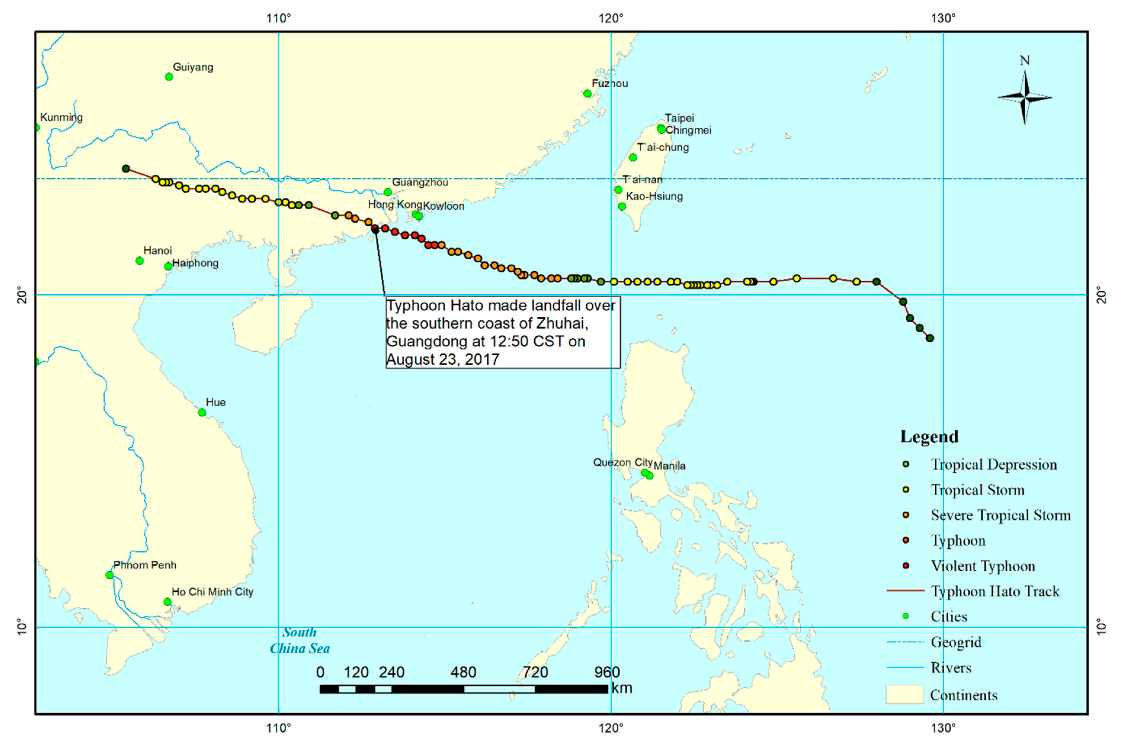
2.1. Case Background

Typhoon Hato (1713) storm surge in the coastal areas of Pearl River estuary in China was taken as a real event study. The Pearl River estuary lies in the Pearl River, the second largest river in China. The estuary is densely covered with river networks, and the Pearl River area is densely populated and economically developed compared to most other parts of China. The region is hit by typhoons frequently, so storm surges bring significant economic losses to the area. Typhoon Hato landed on the coast of Jinwan District, Zhuhai City, Guangdong Province around 12:50 on 23 August 2017. This has been the strongest typhoon landing in the Pearl River estuary since 1965 [35] in terms of the maximum tidal elevation of 2.79 m observed by the Zhuhai station. The typhoon track drawn according to the data provided by the National Meteorological Center is shown in Figure 1.

The largest storm surge occurred in Xiangzhou District, Zhuhai City, in a way of spinning counterclockwise in the northern hemisphere, and the area on the right side of the typhoon track is most seriously affected. Therefore, this paper selected the coastal areas of Macao and Xiangzhou District, Zhuhai City (N 22.06°–N 22.30°, E 113.41°–E 113.60°) as the research area, which were more seriously affected. Topographic data were derived from the ASTGTM dataset provided by the Computer Network Information Center, Chinese Academy of Sciences (CNIC) (http://www.gscloud.cn). ArcGIS 10.5 software (maintained by Esri China Information Technology Co. Ltd. in Beijing, China) was used to preprocess the original data to obtain the range and topographic map of the area, see Figure 2.

The Landsat8 satellite remote sensing data LC81220452018139LGN00 provided by the geospatial data cloud was selected for georeferencing and geometric correction. Because the supervised classification has high precision and controllable classification type, it was selected as the extraction method of land use. The software Arcgis10.5 was imported for cutting and data conversion to obtain the land use distribution map, as shown in Figure 3.

2.2. Initial and Boundary Conditions for Model Testing

The initial and boundary conditions of model testing include three parts, which are the terrain roughness coefficient expressed as the Manning coefficient, the water-level boundary and the definitions of wet and dry. The Manning’s roughness coefficient is another important parameter for calculation of coastal flooding. It reflects the influence of the rough surface of the terrain on the flow of water. Roughness values were associated with the type of surface coverings in different areas. Relative to the impact of terrain on the flood, the surface roughness has less effect on the water level. Only a rough estimate is made here. The Manning’s roughness coefficient of each land use is estimated as follows: development area 0.017, forest 0.16, cropland 0.035, water 0.03, building area 0.015, and the distribution of land use is shown in Figure 3. Besides, the bottom friction coefficient adopts the uniform value (Nikuradse = 0.001). According to the information broadcast by the National Meteorological Center, the duration of typhoon influence in this area was about 8 h, so the simulated flooding process lasted for 8 h (10: 30–18: 30), with a peak hydrographic boundary condition of 2.79 m. The whole simulation was carried out in a closed area. In addition, in order to avoid that fluid retreating from a wet region produces negative water depth that will cause the model to crash. Dry grid cells are defined as cells where h ≤ 0.05 m.

2.3. Methodology

The proposed model is divided into two parts to conduct coastal flooding analysis: (1) a simplified two-dimensional shallow hydrodynamic module that rapidly and accurately simulates the process of the flood inundation; and (2) a risk assessment module that estimates the economic loss by combing the flood data and the land use categories in GIS. In the following subsections, the two parts are discussed in detail.

2.3.1. Simplified Two-Dimensional Shallow Hydrodynamic Module

CA is a grid-based dynamic system, which is discrete in time, space and state, and its spatial interaction and temporal causality are local [26]. It is generally composed of five parts: (1) cells, (2) cellular states, (3) cellular lattice, (4) cellular neighbors, and (5) transformational rules [36].

Traditional triangular mesh generation based on a finite element model can refine and process complex boundaries; however, it is composed of a large amount of data, complex structure and time-consuming calculation, which make it difficult for existing models to couple with other statistical models and carry out a risk analysis in ArcGIS. In this paper, rectangular grid division is used to establish cellular space, which can be easily converted and combined with raster data in spatial structure. The neighborhood structure is the Von Neumann type that consists of the central cell itself and its four adjacent cells, as is shown in Figure 4.

In the CA model, the state of the target cell at the next time steps is determined by both the state of itself and its adjacent cells at the current moment [26]. The core part of CA is to define transformation rules [37]. Therefore, to simulate flood routing more efficiently and accurately, this paper discretizes the two-dimensional shallow hydrodynamic equations and introduces it into the CA model as a transformation rule, in which the spatio-temporal variations in flood depth and velocity are governed by local rules in the neighborhood.

Saint-Venant two-dimensional shallow hydrodynamic Equations with the water depth and flow as main control variables are shown in Equations (1)–(3) [38].

Continuity Equations:

$$\frac{\partial h}{\partial t}+\frac{\partial M}{\partial x}+\frac{\partial N}{\partial y}=0$$

(1)

$$\frac{\partial M}{\partial t}+\frac{\partial \left(uM\right)}{\partial x}+\frac{\partial \left(vM\right)}{\partial y}+gh\frac{\partial Z}{\partial x}+g{n}^{2}u\frac{\sqrt{u^2+v^2}}{\sqrt[3]{h}}=0$$

(2)

$$\frac{\partial N}{\partial t}+\frac{\partial \left(uN\right)}{\partial x}+\frac{\partial \left(vN\right)}{\partial y}+gh\frac{\partial Z}{\partial y}+g{n}^{2}v\frac{\sqrt{u^2+v^2}}{\sqrt[3]{h}}=0$$

(3)

where $h$ is the water depth (m), $Z$ is the water stage (m), $M$ and $N$ are the vertical average unit width discharge in the direction of $x$ and $y$, respectively (m² s⁻¹), $u$ and $v$ are the velocity components of the vertical average velocity in the direction of $x$ and $y$, respectively (ms⁻¹),$n$ is Manning’s roughness coefficient, $t$ is computing time (s) and $g$ is the gravitational acceleration (m/s²).

In momentum equations, the first term is the acceleration term, the second and third are convection terms, the fourth term is the gravity term, and the fifth is the resistance term. The second and third convection ones are nonlinear in differential equations, which often cause instability in calculations and accounts for a relatively small proportion; thus, they can be neglected [38]. In comparison, because of neglecting the convection term in the momentum equation, this greatly reduces the complexity of the equation. Therefore, Equations (1)–(3) are discretized using finite differences and an explicit scheme for the time dependence to obtain Equations (4)–(6). The cellular space difference diagram is shown in Figure 5.

$$\frac{h_{i,j}^{k+1}-h_{i,j}^k}{\mathsf{\Delta }t}+\frac{\left(M_{i+1,j}^k-M_{i,j}^k\right)}{\mathsf{\Delta }x}+\frac{\left(N_{i,j+1}^k-N_{i,j}^k\right)}{\mathsf{\Delta }y}=0$$

(4)

$$\frac{M_{i,j}^{k+1}-M_{i,j}^k}{\mathsf{\Delta }t}+g\frac{\left(h_{i,j}^k+h_{i+1,j}^k\right)\left(Z_{i+1,j}^k-Z_{i,j}^k\right)}{2\mathsf{\Delta }x}+g{n}_{i,j}^2\frac{u_{i,j}^k\sqrt{{\left(u_{i,j}^k\right)}^2+{\left(v_{i,j}^k\right)}^2}}{\sqrt[3]{\left(h_{i,j}^k+h_{i+1,j}^k\right)/2}}=0$$

(5)

$$\frac{N_{i,j}^{k+1}-N_{i,j}^k}{\mathsf{\Delta }t}+g\frac{\left(h_{i,j}^k+h_{i,j+1}^{}\right)\left(Z_{i,j+1}^k-Z_{i,j}^k\right)}{2\mathsf{\Delta }y}+g{n}_{i,j}^2\frac{v_{i,j}^k\sqrt{{\left(u_{i,j}^k\right)}^2+{\left(v_{i,j}^k\right)}^2}}{\sqrt[3]{\left(h_{i,j}^k+h_{i,j+1}^k\right)/2}}=0$$

(6)

In Equations (4)–(6), the computational grid of water depth and velocity is staggered in space and time. Solving Equations (4)–(6) simultaneously, we get Equations (7)–(9), where $k$ is the number of cellular simulation changes, $\mathsf{\Delta }t$ is the size of time step (s), $\mathsf{\Delta }x$ and $\mathsf{\Delta }y$ define the cell size (m), and $i$ and $j$ define the cell position. In the beginning, the water depth and the flow velocity should be initialized ($w$ is the initial flow velocity caused by a typhoon (m s⁻¹)). To meet the convergence and stability conditions, the time step and distance step should be limited, as shown in Equation (10). Therefore, the time step will be adaptive and change during a simulation but is fixed in space at each time step. $c$ is the wave speed (m/s).

$$M_{i,j}^{k+1}=M_{i,j}^k-g\frac{\mathsf{\Delta }t\left(h_{i,j}^k+h_{i+1,j}^k\right)\left(Z_{i+1,j}^k-Z_{i,j}^k\right)}{2\mathsf{\Delta }x}-g{n}_{i,j}^2\frac{u_{i,j}^k\mathsf{\Delta }t\sqrt{{\left(u_{i,j}^k\right)}^2+{\left(v_{i,j}^k\right)}^2}}{\sqrt[3]{\left(h_{i,j}^k+h_{i+1,j}^k\right)/2}}$$

(7)

$$N_{i,j}^{k+1}=N_{i,j}^k-g\frac{\mathsf{\Delta }t\left(h_{i,j}^k+h_{i,j+1}^k\right)\left(Z_{i,j+1}^k-Z_{i,j}^k\right)}{2\mathsf{\Delta }y}-g{n}_{i,j}^2\frac{v_{i,j}^k\mathsf{\Delta }t\sqrt{{\left(u_{i,j}^k\right)}^2+{\left(v_{i,j}^k\right)}^2}}{\sqrt[3]{\left(h_{i,j}^k+h_{i,j+1}^k\right)/2}}$$

(8)

$$h_{i,j}^{k+1}=h_{i,j}^k-\frac{\mathsf{\Delta }t\left(M_{i+1,j}^k-M_{i,j}^k\right)}{\mathsf{\Delta }x}-\frac{\mathsf{\Delta }t\left(N_{i,j+1}^k-N_{i,j}^k\right)}{\mathsf{\Delta }y}$$

(9)

$$\mathsf{\Delta }t\le \frac{\mathsf{\Delta }x}{c}$$

(10)

The cellular state at each moment can be obtained by repeatedly using Equations (7)–(9), assuming $T$ is the total simulation time, the calculation process is shown in Figure 3, where the calculation conditions for assessing the water depth are as follows: according to Equations (7)–(9), when solving for $M$, there is a requirement that at least one water depth state in the x-direction neighborhood of the cell should be greater than zero. Similarly, the calculation condition should be satisfied in the y-direction of the cell.

Based on the above analysis, the algorithm mechanism of the CA model of coastal flooding is as follows: the study area is divided into several rectangular cells with the same size, which make up the cellular space. Each cell in the cellular space has a discrete state and neighborhoods. The state of cellular space itself and its neighborhoods at the current time step determine the cellular state at the next time step, while this process is controlled by the transformation rules. The main algorithm implemented is shown in Figure 6.

The whole simulation process is as follows: first, the original data are entered and the variables are initialized; second, the states of all cells in the cell space are calculated and updated according to the conversion rules, a new round of calculation is started after a one-time step is finished, and the process is repeated until the simulation is completed; finally, the information is the output for subsequent statistical risk analysis, such as the inundation extent, water depth, flow velocity and total duration.

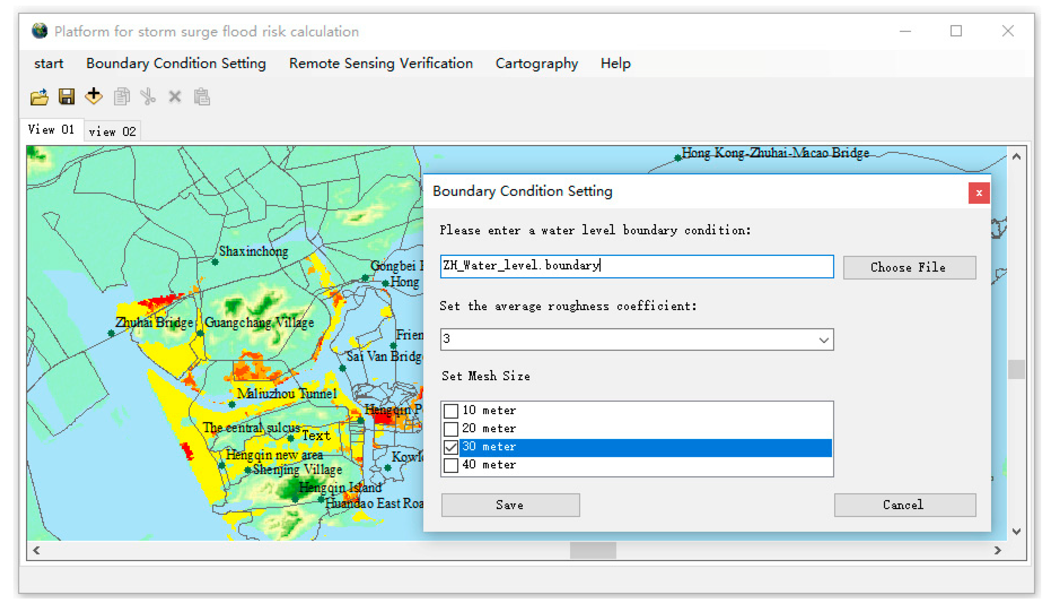
2.3.2. Physically-Based and Real-Time Risk Assessment Module

The quantitative assessment of storm surge disaster loss is the basis and premise of storm surge disaster risk management. Based on the impact of disasters on human survival and development goals, losses can be divided into economic losses and non-economic losses [39]. Economic losses can be further divided into direct economic losses and indirect economic losses. Since the range covered by indirect economic losses is extremely wide, it is very difficult to calculate them thoroughly and accurately. Therefore, in this paper, only direct economic losses are taken into account. According to the land use of the whole area under study, the calculation Equation of direct economic losses is [40]:

$$D_d={\displaystyle \sum _{i=1}^n{\displaystyle \sum _{j=1}^m{D}_{ij}}}={\displaystyle \sum _{i=1}^n{\displaystyle \sum _{j=1}^m{W}_{ij}{\eta }_{ij}}}$$

(11)

where $D_d$ is the total direct economic loss, $D_{ij}$ is the loss value of the i-th disaster-bearing body within the j-th inundation, $W_{ij}$ is the value of the i-th disaster-bearing body within the j-th inundation, ${\eta }_{ij}$ is the loss rate of the i-th disaster-bearing body within the j-th inundation, $n$ is the number of land use, and $m$ is the number of inundation classifications.

The determination of the storm surge disaster loss rate is the key to calculating the economic losses of storm surge disasters. The magnitude of the disaster loss rate is closely related to the disaster situation, the disaster-resistant ability of the disaster bearing body and the moisture-proof measures in the disaster area. In this paper, the disaster loss rate was determined through overlay analysis by studying the historical data of the study area and the loss rate of storm surge disasters in other areas. Land use mainly includes cropland area, forest area, water area, development area and building area. As stated in related reference work [40] and investigated data, the unit area value can be evaluated for the land use. The three types of cropland, forest and water were mainly considered as the economic losses caused by production. The building area was mainly considered the losses of family property, the destruction of houses and basic public facilities. The development area was mainly considered the destruction of houses and basic public facilities, and finally obtained the unit area value of land use.

Table 1. Unit area value of each land use type and the loss rates corresponding to different water depths.

Land Use	Mean	SD	Loss Rate Corresponding to Different Water Depths (%)
	(CNY/m2)	(CNY/m2)	0–0.5	0.5–1.0	1.0–1.5	1.5–2.0	>2.5
Cropland	10.38	2.46	15	25	50	80	100
Water	21.97	4.54	1	2	3	5	7
Forest	0.88	0.23	2	5	10	15	25
Building area	5078.67	1267.44	8	12	17	22	27
Development area	646.94	150.89	3	7	10	14	21

shows the unit area value of each land-use type and the disaster loss rate corresponding to different water depths. In this paper, the unit area value of each land-use type is assumed to follow a normal distribution, with a mean and a standard deviation (SD) (Table 1).

In order to solve the long-standing problem of the integration of hydrodynamic models with large geographic systems. In this paper, by incorporating the flood simulation with geographic statistics and introducing the loss assessment method based on land use, a coupled risk analysis model of coastal flooding was established. To realize the automation of the whole process of storm surge flood disaster analysis, this study adopted a tightly coupled model to integrate the hydrodynamic module and the risk assessment module into the same GIS framework. Thereout, we develop a platform that integrates GIS with hydrological modeling, where the spatiotemporal simulation is integrated with loss analysis of coastal flooding. The platform can intuitively display the flooding process; meanwhile, we can obtain real-time water depth, flow velocity, inundation extent, loss distribution data at different times and so on.

2.3.3. Calibration and Testing

The hydraulic model used for comparison in this article is the HD module in MIKE 21, which is the most well-accepted software for assessing flood hazards in coastal areas [22,23,24]. It uses a two-dimensional hydrodynamic numerical model with an average vertical velocity assumption, for the changes of hydraulic elements such as water depth and flow velocity in the vertical direction are much smaller than the changes in the horizontal direction during the flooding process. It included complex models based on discretized, numerical solutions of general laws (such as the conservation of energy and momentum). The principle has been the idea that sufficient complexity in the model rules was necessary to mimic the complexity of actual flood dynamics. This article intended to discuss from a different perspective, that is spatial complexity can arise in a model with simple rules as long as the spatial interactions of these rules are allowed to be sufficiently complex.

To verify the accuracy and reliability, this paper compared the simulation results of the CA model and MIKE 21 model. Using the data from a real typhoon case, metrics were used to assess the degree of consistency and variation between model predictions, including the inundation extent, two statistics (Root Mean Square Error (RMSE) and Correlation Coefficient (R)) of water-depth data and a comparison of photos of typical sample points.

The RMSE is calculated using Equation (12), where $W_{i,j}^{ca}$ represents the water level simulated by CA at the cell $C_{i,j}$, and $W_{i,j}^{\mathrm{mike}}$ represents the water level simulated by MIKE 21 at the cell $C_{i,j}$. The R statistic is calculated using Equation (13), where $\overline{W_{i,j}^{ca}}$ represents the mean value of water level simulated by CA at the cell $C_{i,j}$, and $\overline{W_{i,j}^{\mathrm{mike}}}$ represents the mean value of water level simulated by MIKE 21 at the cell $C_{i,j}$.

$$RMSE=\sqrt{\frac{{{\displaystyle {\sum }_{i=1,j=1}^{i,j}\left(W_{i,j}^{ca}-W_{i,j}^{\mathrm{mike}}\right)}}^2}{i\times j}}$$

(12)

$$R=\frac{{\displaystyle {\sum }_{i=1,j=1}^{i,j}\left(W_{i,j}^{ca}-\overline{W_{i,j}^{ca}}\right)\left(W_{i,j}^{\mathrm{mike}}-\overline{W_{i,j}^{\mathrm{mike}}}\right)}}{\sqrt{{{\displaystyle {\sum }_{i=1,j=1}^{i,j}\left(W_{i,j}^{ca}-\overline{W_{i,j}^{ca}}\right)}}^2\times {{\displaystyle {\sum }_{i=1,j=1}^{i,j}\left(W_{i,j}^{\mathrm{mike}}-\overline{W_{i,j}^{\mathrm{mike}}}\right)}}^2}}$$

(13)

According to Wang’s research results [41], 300 valid photos were collected from three social media of Weibo, WeChat and Baidu. The photo shooting time, location and water-level information were determined according to the webpage description information and photo display, of which 150 were used for parameter adjustment (MIKE 21 and CA) and 150 for model verification (CA).

3. Results and Discussions

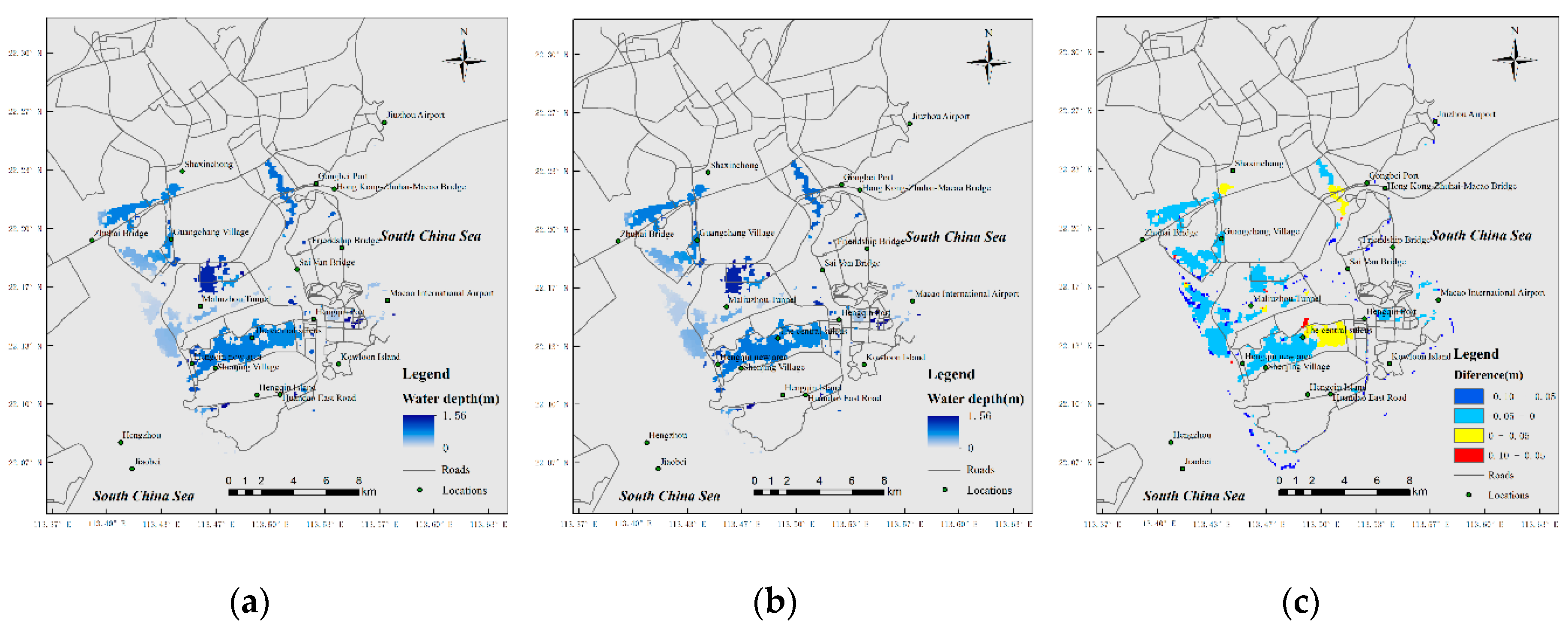
3.1. Comparison with MIKE 21 Simulation Results

The simulation was carried out by using the HD module of MIKE 21, and the model parameters were calibrated to achieve the best simulation effect with the collected 150 social media photos. We adopted the same computational conditions setting for comparing our modeling results and demonstrating the accuracy and efficiency of the proposed model.

The hydraulic elements can be expressed by an average value along the water depth only when the vertical scale of the grid is much smaller than the horizontal scale. The optimal grid size should be between 10 and 200 m. If it is too small, the above conditions cannot be met. If it is too large, the accuracy would be lost. So, the 50 m grid size was taken as an example to illustrate the simulation effect of the CA model. Figure 7, Figure 8 and Figure 9 show the predicted water depths and inundation extent at three time points for both models and the absolute differences in water depth at these times. The inundation extent differs only marginally, and the Root Mean Square Error is only 0.03 m whilst the Correlation Coefficient is 0.95 (see

Table 2. CA model accuracy for maximum inundation of each simulation.

Statistical Parameter	Resolution (m)
	10	25	50	100	200
RMSE (m)	0.02	0.03	0.03	0.04	0.05
R	0.93	0.94	0.95	0.95	0.93

). The maximum differences in water depth are ±0.1 m, but these are very localized and, over the majority of the domain, water depth differences are small. This demonstrates that the CA model is capable of reproducing results that are in agreement with the ones obtained from the MIKE 21. The reason for the discrepancy may be that MIKE 21 computed the full shallow water Equation while CA neglected the convective term, as errors may occur, especially in areas with sudden changes in altitude.

To test whether the model was sensitive to grid size, identical simulations were also run with the MIKE 21 and CA model at $\mathsf{\Delta }x$ = 10, 25, 50, 100 and 200 m (Table 2). It is known from Table 2 that the RMSE of the two models is below 0.05, which demonstrates that the inundation extent and water depth simulated by the CA model are spatially consistent with MIKE 21 results. Besides, their correlation coefficients are higher than 0.93, which illustrates that there is a high correlation and low anomaly between the two model simulation results, which is also reflected in Figure 7, Figure 8 and Figure 9. In summary, the CA model performs well in the study area; in addition, the results are not greatly affected by the grid variation in the defined grid range as the extent of the study area is wide and the terrain slopes gently.

Runtime is an important factor for evaluating the efficiency of the CA model. In this regard, the CA model challenges MIKE 21 in simulating the research area at $\mathsf{\Delta }x$ = 10, 25, 50, 100 and 200 m (see

Table 3. Comparison of simulation time with different grid size.

		Resolution (m)
		10	25	50	100	200
Simulation Time (min)	MIKE	37.02	10.35	3.27	2.60	1.98
	CA	3.58	2.31	1.23	0.71	0.50

). In this comparative analysis, the simulation time of CA was shorter than MIKE 21 by more than 60% for all grid sizes. Furthermore, it needs to be recognized that MIKE 21 needs to carry out mesh processing and define a series of boundary conditions in the early stage, which increases the complexity and workload of the model simulation. The CA model can automatically generate cellular space and intelligently set partial parameters, which helps to realize simple and rapid evaluation of coastal flooding.

3.2. Comparison of CA Model with Social Media-Based Dataset

To evaluate the modeling with the actual water depth, 150 photos were collected from Weibo, WeChat and Baidu for further verification. The water depths were obtained from those photos for a comparison with the CA model at $\mathsf{\Delta }x$ = 10, 25, 50, 100 and 200 m (see

Table 4. CA model accuracy for water level by comparing with a social-media-based dataset.

Collection Channel	Number of Photos
	Total	Correct
		10 m	25 m	50 m	100 m	200 m
Sina-Weibo	50	49	49	49	49	49
WeChat	50	49	49	49	48	48
Baidu	50	48	48	48	48	48

). The results show that errors are low for all grid sizes, but the CA model was marginally better at $\mathsf{\Delta }x$ = 10, 25 and 50 m than $\mathsf{\Delta }x$ = 100 and 200 m, where the solution quality is dominated by the effect of the grid size. To illustrate in detail, five typical location points were selected for a comparison of water depth whose locations are shown in Figure 10 and Figure 11: (a) Baoxi Road (N 22.16°, E 113.48°), (b) Dama Road (N 22.15°, E 113.56°), (c) Honggang Harbor (N 22.16°, E 113.46°), (d) East Dike (N 22.14°, E 113.54°) and (e) Hengqin West Road (N 22.13°, E 113.46°)

According to the photos collected from the typical locations and related reports, it was found that when t = 105 min, the actual water depth of the Dama Road was about 1.1–1.4 m, and the water depth simulated by CA was 1.29 m; when t = 330 min, the actual water depth of the Honggang Harbor was around 0.5–0.8 m, and the water depth simulated by CA was 0.70 m (see Figure 12). Similarly, the water depth in other locations was consistent with the actual situation, illustrating the reliability and accuracy of the CA model. These findings confirm that the CA model can provide a real-time reference in terms of flooding and water depth data for the management of storm surge disasters.

3.3. Coastal Flood Risk Assessment

According to spatial geographic relationships, the maximum water depth data was coupled with land use to preliminarily evaluate the economic losses. The distribution of flood disaster losses in the study area was obtained, and the diagram in the platform interface is shown in Figure 13. The inundation extent and economic losses of land use corresponding to different water depths were counted and shown in

Table 5. Inundation extent and loss value of different land use types corresponding to different water levels.

Water Depth (m)	Cropland		Water		Forest		Building Area		Development Area
	Area (km2)	Loss (104 CNY)	Area (km2)	Loss (104 CNY)	Area (km2)	Loss (104 CNY)	Area (km2)	Loss (108 CNY)	Area (km2)	Loss (108 CNY)
0–0.5	0.33	51.38	9.95	218.60	0.58	1.02	3.34	13.57	1.66	0.32
0.5–1.0	0.44	114.18	7.69	337.90	0.55	2.42	3.16	19.26	1.98	0.90
1.0–1.5	0.35	181.65	5.06	333.50	1.32	11.62	2.31	19.95	2.41	1.56
1.5–2.0	0.33	274.03	3.63	398.76	1.45	19.14	1.55	17.32	2.94	2.66
2.0–2.5	0.33	342.54	5.43	835.08	1.34	29.48	2.00	27.43	6.50	8.83
Total	1.78	963.78	31.76	2123.84	5.24	63.68	12.36	97.53	15.49	14.27

.

$$f_X\left(x\right)=N\left(x;{\mu }_X,{\sigma }_X^2\right)=\frac{1}{\sqrt{2\pi }{\sigma }_X}{e}^{-{\left(x-{\mu }_X\right)}^2/\left(2{\sigma }_X^2\right)}$$

(14)

$$f_Y\left(y\right)=N\left(y;{\mu }_Y,{\sigma }_Y^2\right)=\frac{1}{\sqrt{2\pi }{\sigma }_Y}{e}^{-{\left(y-{\mu }_Y\right)}^2/\left(2{\sigma }_Y^2\right)}$$

(15)

$$f_Z\left(z\right)=N\left(z;{\mu }_Z,{\sigma }_Z^2\right)=\frac{1}{\sqrt{2\pi }{\sigma }_Z}{e}^{-{\left(z-{\mu }_Z\right)}^2/\left(2{\sigma }_Z^2\right)},{\mu }_Z={\mu }_X+{\mu }_Y,{\sigma }_Z=\sqrt{{\sigma }_X^2+{\sigma }_Y^2}$$

(16)

We added up the product of the loss rate and the inundation area for each land use type, and the five sums values were considered as a coefficient in normal distribution functions. Based on the assumption in Section 2.3.2, the probability density distribution of loss for each land use type was calculated. Loss for each land use type is an independent random variable that is normally distributed. Their sum is also normally distributed, which can be derived from Equations (14)–(16) (The sum of two independent normally distributed random variables is normal, with its mean being the sum of the two means, and its variance being the sum of the two variances.) Therefore, the total direct economic loss distribution function and the two relevant parameters (mean loss: CNY 3.17 billion, 95% confidence interval: CNY 1.03~5.32 billion) can be calculated. The actual direct economic loss was CNY 5.15 billion, as reported by the 2017 China Marine Disaster Bulletin [39], which indicates that the model could assess the loss of disasters, especially within an order of magnitude of the error. In the future, we will expand the database and optimize parameters to improve the model.

According to the summary of the data presented in Table 3, the total inundation extent of the study area was 66.63 km². From Figure 13, we can see that the distribution of disaster losses shows a certain regularity: the disaster losses were higher in areas with higher value of per unit area, offshore areas and low marine topography, which reflects the main role of topography, location and unit area value in storm surge flood loss analysis. The order of the losses for each land-use type is as follows: building area > development area > forest > water > cropland. It is obvious that the largest proportion of disaster loss was in the building area. This is mainly because most of the building areas with high investment are located in the low coastal areas, which was severely affected by a storm surge. It can be inferred from Figure 13 and Table 5 that the real-time storm surge monitoring system and emergency plan system in building areas should be improved and strengthened in the process of disaster prevention and mitigation, and that the dike construction along the coastal areas should also be strengthened.

4. Conclusions

This study outlines a new model that integrates a hydrodynamic module and a risk assessment module for flood simulation and risk assessment in the coastal areas of the Pearl River estuary, China. The hydrodynamic module that based on the CA model, the effectiveness of which has been demonstrated by comparing the simulation results with MIKE 21 and a social-media-based dataset. Then, the simulated water depth and land-use data are utilized to estimate the storm surge risk that was visualized on the integrated platform.

The CA model in this study well simulates the historical storm events with good confidence and accuracy when comparing with MIKE 21 and a social-media-based dataset. In terms of the inundation data at three different times, the inundation and difference of the two models were drawn at a grid size of 50 m. Moreover, the RMSE (≤0.05 m) and R (≥0.93) were calculated at $\mathsf{\Delta }x$ = 10, 25, 50, 100 and 200 m. The results show a little discrepancy of two models but that is reasonable. Similarly, the water depth obtained from the CA model was consistent with depth data from a social-media-based dataset at five grid sizes. The results clearly illustrate that the CA model performed well for the entire study area. At the same time, the simulation time of the CA model was over 60% shorter than that of MIKE 21, achieving a fast computational performance with high accuracy.

Analyzing flood risk, the results indicate that the total inundation extent of the study area was 66.63 km², and the direct economic losses were 11.40 billion CNY, which is very close to the actual losses incurred and thus demonstrates computational reliability. They reflect the main role of topography, location and unit area value in storm surge flood risk analysis. Moreover, based on the GIS framework, this study integrated the hydrodynamic module with the statistical risk analysis model with a tight coupling, designing and developing a data-driven automatic assessment platform for coastal flood risk. It realized a refined risk assessment of coastal flood and will provide strong theoretical guidance and technical support for future storm surge disaster risk analysis and the development of disaster prevention measures.

The CA model established in this paper adopts the same cellular unit and neighborhood definition in the whole simulation process. Future work could improve the model to automatically adjust the grid division and select the neighborhood types according to the terrain complexity, and introduce a data assimilation algorithm to calibrate the model parameters. The spatio-temporal dynamic evolution of geographic phenomena and spatial heterogeneity of velocity can be introduced into the cellular automata model, which can improve the simulation of the spatio-temporal dynamic process of geographical phenomena. Moreover, the combination of cellular automata and parallel algorithms to improve the computational efficiency and analyze the uncertainty of the flood disaster loss assessment and the difference in multiple scenarios (e.g., Dike breach, climate change) could be the focus of future research.

References

1. Hallegatte, S.; Green, C.; Nicholls, R.; Corfee-Morlot, J. Future flood losses in major coastal cities. Nat. Clim. Chang. 2013, 3, 802–806. [Google Scholar] [CrossRef]
2. Burrus, R.; Dumas, C.; Graham, J. Hurricane risk and coastal property owner choices. Int. J. Disaster. Resil. Built. Environ. 2011, 2, 118–138. [Google Scholar] [CrossRef] [Green Version]
3. Klerk, W.J.; Winsemius, H.C.; Van Verseveld, W.J.; Bakker, A.M.R.; Diermanse, F.L.M. The co-incidence of storm surges and extreme discharges within the Rhine–Meuse Delta. Environ. Res. Lett. 2015, 10, 035005. [Google Scholar] [CrossRef] [Green Version]
4. Vousdoukas, M.; Voukouvalas, E.; Annunziato, A.; Giardino, A.; Feyen, L. Projections of extreme storm surge levels along Europe. Clim. Dyn. 2016, 47, 3171–3190. [Google Scholar] [CrossRef] [Green Version]
5. Androulidakis, Y.; Kombiadou, K.; Makris, C.; Baltikas, V.; Krestenitis, Y. Storm surges in the mediterranean sea: Variability and trends under future climatic conditions. Dyn. Atmos. Oceans. 2015, 71, 56–82. [Google Scholar] [CrossRef]
6. Lin, N.; Emanuel, K. Grey swan tropical cyclones. Nat. Clim. Chang. 2015, 6, 106–111. [Google Scholar] [CrossRef] [Green Version]
7. Schubert, C.E.; Busciolano, R.J.; Hearn, P.P.; Rahav, A.N.; Behrens, R.; Finkelstein, J.S.; Monti, J.; Simonson, A.E. Analysis of storm-tide impacts from Hurricane Sandy in New York. Available online: https://pubs.er.usgs.gov/publication/sir20155036 (accessed on 26 September 2019).
8. Poulter, B.; Halpin, P. Raster modelling of coastal flooding from sea-level rise. Int. J. Geogr. Inf. Sci. 2008, 22, 167–182. [Google Scholar] [CrossRef]
9. Lichter, M.; Felsenstein, D. Assessing the costs of sea-level rise and extreme flooding at the local level: A GIS-based approach. Ocean Coastal Manag. 2012, 59, 47–62. [Google Scholar] [CrossRef]
10. Aerts, J.; Lin, N.; Botzen, W.; Emanuel, K.; de Moel, H. Low-probability flood risk modeling for New York City. Risk Anal. 2013, 33, 772–788. [Google Scholar] [CrossRef]
11. Lloyd, S.; Kovats, R.; Chalabi, Z.; Brown, S.; Nicholls, R. Modelling the influences of climate change-associated sea-level rise and socioeconomic development on future storm surge mortality. Clim. Chang. 2015, 134, 441–455. [Google Scholar] [CrossRef]
12. Gallien, T.; Schubert, J.; Sanders, B. Predicting tidal flooding of urbanized embayments: A modeling framework and data requirements. Coast. Eng. 2011, 58, 567–577. [Google Scholar] [CrossRef]
13. Ramirez, J.; Lichter, M.; Coulthard, T.; Skinner, C. Hyper-resolution mapping of regional storm surge and tide flooding: Comparison of static and dynamic models. Nat. Hazards. 2016, 82, 571–590. [Google Scholar] [CrossRef]
14. Bates, P.; Horritt, M.; Fewtrell, T. A simple inertial formulation of the shallow water equations for efficient two-dimensional flood inundation modelling. J. Hydrol. 2010, 387, 33–45. [Google Scholar] [CrossRef]
15. Patro, S.; Chatterjee, C.; Mohanty, S.; Singh, R.; Raghuwanshi, N. Flood inundation modeling using MIKE FLOOD and remote sensing data. J. Indian Soc. Remote Sens. 2009, 37, 107–118. [Google Scholar] [CrossRef]
16. Xia, J.; Guo, P.; Zhou, M.; Falconer, R.; Wang, Z.; Chen, Q. Modelling of flood risks to people and property in a flood diversion zone. J. Zhejiang Univ.-Sci. A 2018, 19, 864–877. [Google Scholar] [CrossRef]
17. Prakash, M.; Rothauge, K.; Cleary, P. Modelling the impact of dam failure scenarios on flood inundation using SPH. Appl. Math. Model. 2014, 38, 5515–5534. [Google Scholar] [CrossRef]
18. Vacondio, R.; Rogers, B.; Stansby, P.; Mignosa, P. SPH modeling of shallow flow with open boundaries for practical flood simulation. J. Hydraul. Eng.-ASCE 2012, 138, 530–541. [Google Scholar] [CrossRef]
19. Wang, X.; Sun, X.; Zhang, S.; Sun, R.; Li, R.; Zhu, Z. 3D simulation of storm surge disaster based on scenario analysis. Trans. Tianjin Univ. 2016, 22, 110–120. [Google Scholar] [CrossRef]
20. A State of the Art Review on Mathematical Modelling of Flood Propagation. Available online: http://www.impact-project.net/cd/papers/print/008_pr_02-05-16_IMPACT_Alcrudo.pdf (accessed on 30 May 2020).
21. McLusky, D.; Wolanski, E. Treatise on Estuarine and Coastal Science; Academic Press: Amsterdam, The Netherlands, 2011; pp. 441–458. [Google Scholar]
22. Warren, I.; Bach, H. MIKE 21: A modelling system for estuaries, coastal waters and seas. Environ. Softw. 1992, 7, 229–240. [Google Scholar] [CrossRef]
23. Madsen, H.; Jakobsen, F. Cyclone induced storm surge and flood forecasting in the northern Bay of Bengal. Coast. Eng. 2004, 51, 277–296. [Google Scholar] [CrossRef]
24. Wang, J.; Gao, W.; Xu, S.; Yu, L. Evaluation of the combined risk of sea level rise, land subsidence, and storm surges on the coastal areas of Shanghai, China. Clim. Chang. 2012, 115, 537–558. [Google Scholar] [CrossRef]
25. Wolfram, S. Computation theory of cellular automata. Commun. Math. Phys. 1984, 96, 15–57. [Google Scholar] [CrossRef]
26. Zhou, C.; Sun, Z.; Xie, Y. Research of Geographical Cellular Automata; Science Press: Beijing, China, 1999. (In Chinese) [Google Scholar]
27. Murray, A.; Paola, C. A cellular model of braided rivers. Nature 1994, 371, 54–57. [Google Scholar] [CrossRef]
28. Folino, G.; Mendicino, G.; Senatore, A.; Spezzano, G.; Straface, S. A model based on cellular automata for the parallel simulation of 3D unsaturated flow. Parallel Comput. 2006, 32, 357–376. [Google Scholar] [CrossRef]
29. Mendicino, G.; Senatore, A.; Spezzano, G.; Straface, S. Three-dimensional unsaturated flow modeling using cellular automata. Water Resour. Res. 2006, 42. [Google Scholar] [CrossRef]
30. Cai, X.; Li, Y.; Wu, W.; Wang, Y. Cellular automaton model of flood submergence based on bulk method. J. Hydroelectric. Eng. 2013, 32, 30–34. (In Chinese) [Google Scholar]
31. Li, Y.; Gong, J.; Zhu, J.; Song, Y.; Hu, Y.; Ye, L. Spatiotemporal simulation and risk analysis of dam-break flooding based on cellular automata. Int. J. Geogr. Inf. Sci. 2013, 27, 2043–2059. [Google Scholar] [CrossRef]
32. Guidolin, M.; Chen, A.; Ghimire, B.; Keedwell, E.; Djordjević, S.; Savić, D. A weighted cellular automata 2D inundation model for rapid flood analysis. Environ. Modell. Softw. 2016, 84, 378–394. [Google Scholar] [CrossRef] [Green Version]
33. Dottori, F.; Todini, E. Developments of a flood inundation model based on the cellular automata approach: Testing different methods to improve model performance. Phys. Chem. Earth 2011, 36, 266–280. [Google Scholar] [CrossRef]
34. Parsons, J.; Fonstad, M. A cellular automata model of surface water flow. Hydrol. Process. 2007, 21, 2189–2195. [Google Scholar] [CrossRef]
35. 2017 State Oceanic Administration. Available online: http://gc.mnr.gov.cn/201806/t20180619_1798021.html (accessed on 30 May 2020).
36. White, R.; Engelen, G. High resolution integrated modeling of the spatial dynamics of urban and regional systems. Comput. Environ. Urban Syst. 2000, 24, 383–400. [Google Scholar] [CrossRef] [Green Version]
37. Li, X. Geographic Simulation System: Cellular Automata and Multi-Agent; Science Press: Beijing, China, 2007. (In Chinese) [Google Scholar]
38. Liu, S.K.; Li, X.; Li, S.; Yu, T. Numerical simulation of flood routing in Xiaoqinghe plain. Shuikexue Jinzhan 1991, 2, 188–193. (In Chinese) [Google Scholar]
39. Merz, B.; Kreibich, H.; Schwarze, R.; Thieken, A. Review Article “Assessment of economic flood damage”. Nat. Hazards Earth Syst. Sci. 2010, 10, 1697–1724. [Google Scholar] [CrossRef]
40. Wei, Y.M.; Jin, J.L.; Yang, C.J.; Huang, S.F.; Fan, Y.; Chen, D.Q. Theory of Risk Management of Flood Disaster; Science Press: Beijing, China, 2020. (In Chinese) [Google Scholar]
41. Yang, T.; Xie, J.; Li, G. A Social Media-based Dataset of Typhoon Disasters. 2017. Available online: http://www.scidb.cn/detail?dataSetId=633694461024534528&language=zh_CN&dataSetType=journal (accessed on 14 April 2020).
Figure 1. Track of Typhoon Hato.
Water 12 02076 g001
Figure 2. Location of the study area. (a) Administrative map of China; (b) map of Guangdong Province; (c) topographic map of the study area; (d) remote sensing map of the study area.
Water 12 02076 g002
Figure 3. Distribution map of land use in the study area.
Water 12 02076 g003
Figure 4. Von-Neumann-type neighborhood.
Water 12 02076 g004
Figure 5. Cellular space difference.
Water 12 02076 g005
Figure 6. Flowchart of the cellular automata (CA) model calculation.
Water 12 02076 g006
Figure 7. Inundation estimated by (a) MIKE 21 and (b) the CA simulated inundation, and (c) their difference (MIKE 21-CA) at 120 min.
Water 12 02076 g007
Figure 8. Inundation estimated by (a) MIKE 21 and (b) the CA simulated inundation, and (c) their difference (MIKE 21-CA) at 240 min.
Water 12 02076 g008
Figure 9. Inundation estimated by (a) MIKE 21 and (b) the CA simulated inundation, and (c) their difference (MIKE 21-CA) at 480 min.
Water 12 02076 g009
Figure 10. Photos of typical locations. (a) Honggang Harbor, t = 330 min (16:00); (b) Hengqin West Road, t = 115 min (12:25); (c) Baoxi Road, t = 140 min (12:50); (d) East Dike, t = 300 min (15:30); (e) Dama Road, t = 105 min (12:15).
Water 12 02076 g010
Figure 11. Five typical locations.
Water 12 02076 g011
Figure 12. Water-level variation curve at typical locations.
Water 12 02076 g012
Figure 13. Distribution of flood disaster losses map on the platform interface.
Water 12 02076 g013