Article

Urban Flood Modeling Using 2D Shallow-Water Equations in Ouagadougou, Burkina Faso

International Institute for Water and Environmental Engineering (2iE), Rue de la science-01, P.O. Box 594, Ouagadougou, Burkina Faso
*
Authors to whom correspondence should be addressed.
Water 2020, 12(8), 2120; https://doi.org/10.3390/w12082120
Submission received: 31 May 2020 / Revised: 14 July 2020 / Accepted: 19 July 2020 / Published: 26 July 2020
(This article belongs to the Special Issue Urban Water Management and Urban Flooding)

Abstract

:
Appropriate methods and tools accessibility for bi-dimensional flow simulation leads to their weak use for floods assessment and forecasting in West African countries, particularly in urban areas where huge losses of life and property are recorded. To mitigate flood risks or to elaborate flood adaptation strategies, there is a need for scientific information on flood events. This paper focuses on a numerical tool developed for urban inundation extent simulation due to extreme tropical rainfall in Ouagadougou city. Two-dimensional (2D) shallow-water equations are solved using a finite volume method with a Harten, Lax, Van Leer (HLL) numerical fluxes approach. The Digital Elevation Model provided by NASA’s Shuttle Radar Topography Mission (SRTM) was used as the main input of the model. The results have shown the capability of the numerical tool developed to simulate flow depths in natural watercourses. The sensitivity of the model to rainfall intensity and soil roughness coefficient was highlighted through flood spatial extent and water depth at the outlet of the watershed. The performance of the model was assessed through the simulation of two flood events, with satisfactory values of the Nash–Sutcliffe criterion of 0.61 and 0.69. The study is expected to be useful for flood managers and decision makers in assessing flood hazard and vulnerability.

Graphical Abstract

1. Introduction

In human history, natural disasters have always existed as a common and recurrent phenomenon. Among them, floods are the most widespread worldwide disaster and appear at the top ranking due to important fatalities and damages caused [1,2,3]. According to the United Nations International Strategy for Disaster Reduction [4], flood disasters account for about one-third of all-natural disasters, ranking by economic losses, between 1994 and 2013. The occurrence of flood events in many parts of the world has raised public, political, and scientific interest in flood risks and prevention strategies [5,6]. Despite considerable technologies developed for forecasting, management, and defense, floods are still a significant threat around the world [7]. In a recent study, Petrucci et al. [7], showed that 812 floods recorded killed 2466 people, with important losses, based on 39 years (between 1980 and 2018) of recorded data over nine study areas located in Europe.
In recent decades, Sahelian countries have been strongly affected by high-impact weather events. For example, heavy rains in 2018 affected more than 200,000 victims and caused 52 deaths, where Niamey and its vicinity was the hardest hit area [8]. In addition, this extreme event killed thousands of livestock and destroyed more than 170,000 houses and almost 8000 hectares of crops. In 2009, flooding affected 600,000 people in 12 West African countries, resulting in 193 deaths. The hardest-hit countries were Burkina Faso, Senegal, Ghana, and Niger [9]. Unfortunately, future climate projections over West Africa converge on the possibility of greater magnitudes and more frequent floods, due to extreme events [10,11,12,13,14,15,16]. Urban areas are particularly more vulnerable to floods. Indeed, for large Sahelian cities like Ouagadougou, Niamey, or Dakar, due to high population growth [17,18], rapid and uncontrolled urbanization, and insufficient or a lack of drainage systems [19], the number of flood events has increased, with severe damages [20,21].
Many studies [1,22,23,24] have been devoted to understanding the causes of floods in Sahelian countries and to minimize the consequences of floods. According to Descroix et al. [25], anthropogenic drivers and climate change are considered the principal causes of flood generation. In the Niamey region of the Niger basin, land clearing and population settlements contribute to amplifying the magnitude of flood events. However, Taylor et al. [13] and Wilcox et al. [14] pointed out that the magnitude of floods and the high fatalities observed in Sahelian areas are related to extreme rain events due to global climate change. Tazen et al. [26] showed that land-use change, especially in urban areas, contributes to an increase in the frequency of flooding.
The perception of floods and mitigation actions by flood victims in the Sahel have been elucidated by [24,27]. Flood risk management in urban areas is a key issue for governments in the Sahel countries [22,28]. To strengthen the resilience of urban areas and minimize economic losses, it is necessary to develop participatory disaster management systems through community-based projects. Several structural and non-structural measures have been adopted by policymakers to minimize flood damage in urban areas. In Sahelian countries, for instance, since the 1950s the majority of towns were built around watercourses, without clear drainage systems and urbanization plans. Unfortunately, these measures seem to be ineffective [6,21,27]. Given the occurrence of flood events, it becomes imperative to implement new approaches that should be able to better characterize flow discharges in urban areas.
During the two last centuries, scientists and engineers have developed numerical models to describe water flow behavior [29,30]. Various tools (e.g., LISFLOOD-FP [31]; Rubar 20 code [32,33], MIKE software (Danish Hydraulic Institute); HEC-RAS) based on mechanistic models have been used to simulate flooding in cities worldwide. Urban flows have been described in many studies [29,34,35,36,37] using either one-dimensional (1D), two-dimensional (2D), or three-dimensional (3D) approaches that have been obtained by approximation through hypothesis from Navier–Stokes (NS) equations. Models based on Saint-Venant equations are adapted to describe flow in shallow water conditions [31,33,38]. Some authors have successfully coupled hydrodynamic (1D–2D) model [39,40] approaches as an improvement of urban flood simulation, while others [41,42,43] have used hydrodynamic models coupled with hydrological models for the same purpose, to take into account the runoff generation processes. According to Bellos et al. [42], most of the recent applications of hydrodynamics models agree on an accuracy of 2D models for urban flood modeling. Although these tools for flow simulation exist and are extensively used around the world, the cost of their implementation and the quality of the input data required limit their use in developing countries, particularly for flood management purposes. The choice of a 2D model of Saint-Venant equations for this study can be explained by several reasons. Based on conservation laws of mass and momentum fluid particles, equations are solved by representing flows in Cartesian (x, y) directions. Thus, the spatial distribution of rainfall, topography, and runoff processes in urbanized area, such as the influence of soil roughness and infiltration, can be taken into account. There is an issue in the numerical resolution of this model in terms of equilibrium instabilities due to topography variation and a time-splitting scheme. To overcome these constraints, the well known and widely applied HLL scheme has been adopted. The HLL scheme was used to approximate the flow at cell interfaces. By reconstructing the hydrostatic height of water in the approximation, it can eliminate instabilities related to topography. The time-step is then recalculated at the end of each iteration to guarantee the stability of the solution. This study approach has never been applied for flood management in Ouagadougou, despite important damage recorded each year.
This study aimed to develop a 2D hydraulic model for urban flood extent mapping. The finite volume scheme approach [44] was used to numerically solve shallow-water equations. The performance of the numerical tool developed was appreciated through the simulation of some real flood events observed in a peri-urban watershed in the city of Ouagadougou.
This paper is structured as follows: Section 2 gives a description of the study area, and Section 3 describes the mathematical formalism of flow dynamics in the shallow water, the numerical resolution scheme used, and the input data for application. Section 4 presents the results of the sensitivity analysis and outputs from simulations of real cases of flood events. The conclusions of this study are summarized in Section 5.

2. Materials and Methods

2.1. Study Area

Ouagadougou, the capital city in Burkina Faso (Figure 1), records important damages linked to floods almost each year. Ouagadougou town has three (3) reservoirs (dams) built since 1963 over Masili river, which drain into the Nakanbe river. A small peri-urban watershed in Ouagadougou was selected for this study because of important damages linked to floods each year and mainly because for two years (2016–2017), flow data monitored at a sub-hourly time scale (15 min) is available. This watershed at the outlet (Latitude 12°18 , Longitude −1°26 ) covers a surface area of 75 km2, with almost 47% of the total area covered by urban settlements (Figure 1b). It is drained by intermittent tributaries of the Massili River. The topographic elevation ranges from 287 to 334 m, with a global slope of 1.45 m/km. The study area is located in a Soudano–Sahelian climate, and the mean annual precipitation is about 788 mm (1961–2015). For that same period, the average daily minimum temperature was 16 °C (Harmattan in December) and the daily maximum temperature was 40 °C in April. In this watershed, there are presidential, industrial, and commercial zones. The population in this zone is estimated at 387,000 inhabitants (estimation in 2020).

2.2. Two-Dimensional (2D) Flood Inundation Modeling

Overland surface-flow routing in an urban area is usually simulated by a two-dimensional model [5,32,33] in a wide range of various flow conditions [30] including floods events due to dam failures, heavy rainfall, tidal hydrodynamics, and ocean tsunami hazards. For flood management purposes, this study focused on the estimation of flood patterns (flood extent and flood depth) in a peri-urban area. To achieve this objective, the 2D model seems to be appropriate for this application. According to Alcrudo et al. [36], for such an application, four (4) main steps should be fulfilled for flood propagation model development. These are: (i) understanding of the flow processes relative to the problem; (ii) formulation of appropriate mathematical laws; (iii) development of numerical techniques to solve them and; (iv) validation of model output against experimental and real-life data. The developed model processes are described as follow based on assumptions made by Alcrudo et al. [36].

2.2.1. Mathematical Model Description

The Saint-Venant equations are derived from the laws of conservation of mass and momentum [31,36]. These equations in vector formulation are stated as
U t + F ( U ) x + G ( U ) y = S z + S f + S p ,
where U = ( h , h u , h v ) T represents the vector of conservative unknowns. The variables x [m] and y [m] are the space coordinates of any flow particle in the soil surface. t [s] represents the time variable. The variables h [m], u [m/s], and v [m/s] defined at each point ( x , y ) represent, respectively, the water depth under the reference plane, the velocity component in the x direction, and the velocity in the y direction. The variables in Equation (1) are defined below:
  • The functions F and G represent the advective and pressure fluxes, respectively, in the x and y directions:
    F ( U ) = ( h u , h u 2 + 1 2 g h 2 , h u v ) T , G ( U ) = ( h v , h u v , h v 2 + 1 2 g h 2 ) T .
  • The terms S z and S f designate, respectively, the bottom slope and the friction terms:
    S z = ( 0 , g h z x , g h z y ) T , S f = ( 0 , S f x , S f y ) T .
    g [m/s2] represents the gravitational acceleration and z ( x , y ) [m] define the soil elevation. Friction terms are computed using Manning’s formula [38]:
    S f x = n 2 u 2 + v 2 h 4 / 3 u , S f y = n 2 u 2 + v 2 h 4 / 3 v ,
    where n [m 1 / 3 /s] is the Manning–Strickler coefficient, which characterizes the soil roughness.
  • S p represents the source term stated as:
    S p = ( P I , 0 , 0 ) T ,
    where P [m/s] and I [m/s] are, respectively, the rainfall intensity and infiltration rate. The infiltration rate was estimated using Horton’s model [38]. It is the process of water entrance through the soil profile, and its rate decreases during the rainfall event.
    I ( t ) = i f + ( i 0 i f ) exp ( r t ) ,
    where i 0 [m/s], i f [m/s], and r [s 1 ] are, respectively, the initial infiltration rate, the final infiltration rate, and a constant depending on soil properties.
In this study, the real evapotranspiration is neglected due to the fact that it is an event-based model. It is considered that during the extreme rain event, the real evapotranspiration is very low compared to the volume of precipitation. The model developed uses a structured grid to describe distributed watershed characteristics including topography, urbanization, soil type, and so on. In this model, physical processes of runoff generation are integrated, and particularly, rainfall runoff and infiltration processes are considered over each single grid cell.

2.2.2. Model Numerical Resolution

The model is solved numerically with the finite volume method in a structured grid, hence ensuring proper mass and momentum conservation [45,46]. The geometry of domain Ω is replaced by a structured mesh, where the nodes (grid cell centers) are indexed by integers i and j, respectively, in the x and y axis. The spacing between successive nodes is equal and denoted by Δ x in the x-axis and Δ y in the y-axis.

2.2.3. Grid and Numerical Scheme

The computational grids of domain consist of interior cells that are labeled by i = 1; 2; ⋯; m x and j = 1; 2; ⋯; m y (Figure 2). The grid is extended by setting a set of two ghost cells at all sides, for i = 1 ; 0 and i = m x + 1; m x + 2, and for j = 1 ; 0 and j = m y + 1; m y + 2. At the beginning of each time step, the ghost-cell values are filled based on data in the interior cells and the given boundary conditions. The computational domain is assumed to be large enough, so that there will be only outgoing waves on the boundary of this domain. Hence, along the boundary edge, we set:
U 1 , j = U 0 , j = U 1 j , U m x + 1 , j = U m x + 2 , j = U m x , j , j = 1 , , m y , U i , 1 = U i , 0 = U i , 1 , U i , m y + 1 = U i , m y + 2 = U i , m y , i = 1 , , m x .
The resolution in time is split into a sequence of one-dimensional problems.
(a)
In the x-sweeps, we start with a solution U i , j n along each row of cells C i , j , with j fixed. The numerical solution at time t n + 1 4 is obtained from the resolution of the following scheme:
U i , j n + 1 / 4 U i , j n Δ t + F i + 1 / 2 , j n F i 1 / 2 , j n Δ x = 0 ,
where F i 1 / 2 , j n is an appropriate numerical flux between cells C i 1 , j and C i , j .
(b)
In the y-sweeps, we use the values of U i , j n + 1 / 4 as data along each column of cells, with i fixed. That results in the calculation of the solution at time t n + 2 / 4 , from the scheme
U i , j n + 2 / 4 U i , j n + 1 / 4 Δ t + G i , j + 1 / 2 n + 1 / 4 G i , j 1 / 2 n + 1 / 4 Δ y = 0 ,
where G i , j 1 / 2 n + 1 / 4 is an appropriate numerical flux between cells C i , j 1 and C i j .
(c)
Friction and source terms (rainfall, infiltration, ...) are taken into account using the two following schemes:
U i , j n + 3 / 4 U i , j n + 2 / 4 Δ t = S f ( U i , j n + 2 / 4 ) , U i , j n + 1 U i , j n + 3 / 4 Δ t = S p ( U i , j n + 3 / 4 ) .

2.2.4. Hydrostatic Reconstruction

The HLL approximation [46] presented above is used to build the numerical fluxes at the cell interfaces. Moreover, the water height is reconstructed in order to preserve equilibrium states [44].
(i) 
The fluxes in the x-axis at the right and left of cell C i , j are defined by
F i + 1 / 2 , j n = F ( U i + 1 / 2 , j n , U i + 1 / 2 + , j n ) g α + 2 2 e y , F i 1 / 2 , j n = F ( U i 1 / 2 , j n , U i 1 / 2 + , j n ) g α 2 2 e y ,
where e y = ( 0 , 1 , 0 ) T . The reconstructed solution at the interfaces is defined by
U i + 1 / 2 , j = α ( 1 , u i , j , v i , j ) T , U i + 1 / 2 + , j = α + ( 1 , u i + 1 , j , v i , j ) T ,
with
z i + 1 / 2 , j = max ( z i , j , z i + 1 , j ) , α + = max ( h i , j + z i , j z i + 1 / 2 , j , 0 ) , α = max ( h i , j + z i , j z i 1 / 2 , j , 0 ) .
(ii) 
The fluxes in the y-axis above and under cell C i , j are defined by
G i , j + 1 / 2 n = G ( U i , j + 1 / 2 n , U i , j + 1 / 2 + n ) g α 2 2 e z , G i , j 1 / 2 n = G ( U i , j 1 / 2 n , U i , j 1 / 2 + n ) g α + 2 2 e z ,
where e z = ( 0 , 0 , 1 ) T . The reconstructed solution at the interfaces is defined by
U i , j + 1 / 2 = α ( 1 , u i , j , v i , j ) T , U i , j + 1 / 2 + = α + ( 1 , u i , j , v i , j + 1 ) T ,
with
z i , j + 1 / 2 = max ( z i , j , z i , j + 1 ) , α = max ( h i , j + z i , j z i , j + 1 / 2 , 0 ) , α + = max ( h i , j + 1 + z i , j + 1 z i , j + 1 / 2 , 0 ) .

2.2.5. Flux at Cell Interfaces

The fluxes F and G are computed by HLL approximation developed by Harten, Lax, and Van Leer [44,47,48,49]. Following this HLL scheme, the upwind direction of each term of the fluxes is simply dictated by the sign of the flow velocity reconstructed at the interface of the cells. The HLL fluxes at cell interfaces are expressed as follows:
F ( U G , U D ) = F ( U G ) if 0 c 1 x , c 2 x F ( U G ) c 1 x F ( U D ) + c 1 x c 2 x ( U D U G ) c 2 x c 1 x if c 1 x < 0 < c 2 x , F ( U D ) if c 2 x 0 ,
G ( U B , U H ) = G ( U B ) if 0 c 1 y , c 2 y G ( U B ) c 1 y G ( U H ) + c 1 y c 2 y ( U H U B ) c 2 y c 1 y if c 1 y < 0 < c 2 y , G ( U H ) if c 2 y 0 ,
where U G , U D , U B , and U U are, respectively, the left, right, down, and up approximations of the solution at the current cell. The coefficients c i x , c i y , i = 1 , 2 are defined by
c 1 x = min U = U G , U D min j = 1 , 2 , 3 λ j x ( U ) , c 2 x = max U = U G , U D max j = 1 , 2 , 3 λ j x ( U ) , c 1 y = min U = U B , U H min j = 1 , 2 , 3 λ j y ( U ) , c 2 y = max U = U B , U H max j = 1 , 2 , 3 λ j y ( U ) .
The terms λ i x and λ i y , i = 1 , 2 , 3 are, respectively, the eigenvalues of the Jacobian of F and G. They are defined by
λ 1 x = u g h , λ 2 x = u , λ 3 x = u + g h , λ 1 y = v g h , λ 2 y = v , λ 3 y = v + g h .
The numerical solution at the grid cell indexed by ( i , j ) , at time t n , is the approximation
U i , j n 1 Δ x Δ y y j 1 / 2 y j + 1 / 2 x i 1 / 2 x i + 1 / 2 U ( x , y , t n ) d x d y .

3. Application to a Peri-Urban Watershed in Ouagadougou

The model described above is applied to a small peri-urban watershed located in Ouagadougou, Burkina Faso (Figure 1). Some input data are needed to build and to evaluate a numerical model. In general, four types of information are required: i—topographical data for the description of the geometry of the study area; ii—hydrometric observations for the definition of initial and boundary conditions; iii—effective friction and infiltration parameters for each grid cell; and iv—hydrographs for model validation.

3.1. Model Input Data

3.1.1. Digital Elevation Model or Topographic Data

The calculation of overland flow and the estimation of the flooded areas require elevation information of the watershed. To simulate the hydrologic processes on the watershed, topographic data or the Digital Elevation Model (DEM) was downloaded from USGS (U.S Geological Survey) website (https://earthexplorer.usgs.gov/), with a spatial resolution of 30 m. From the DEM, regular square grids were built including the area of interest. The coordinates system has been reset based on the lowest values of longitude and latitude coordinates. Thus, 409 × 409 nodes were obtained over the study domain. This topographic data with grid nodes is presented in Figure 3.

3.1.2. Roughness and Infiltration Parameters

Roughness and infiltration rates are influenced by many factors such as soil type, soil moisture, land cover, and land use, among others. Land cover and land use classification data were provided by the Burkina Faso National Institute of Geography (IGB, http://www.igb.bf/). After re-projection, re-sampling, and extraction of land-use classes, these data were overlayed with the watershed grid system. Manning’s roughness values were selected from the published literature [50,51,52,53]. Roughness parameters and those of infiltration were collected from the scientific literature because the land-use types considered for our study area are similar to those found in the literature. The values used could be similar to those from field measurements. The roughness values for the overland surface grid cells and interception storage capacity were specified based on land-use classes in Table 1. Likewise, the infiltration map was elaborated by taking into account the maximum infiltration rate of different land cover given in Table 2. Model scenarios were built upon information from Table 1 and Table 2.

3.1.3. Rainfall and Water Depth Data

To build the model, synthetic rainfall data were prepared to analyze the model sensitivity to this input variable with the hypothesis of rainfall uniformity over the watershed. To evaluate the model, two real cases of rain events in 2016 were used. Rainfall and flow data used in this study were collected in the framework of AMMA-2050 (https://www.amma2050.org/) project activities.

3.2. Model Sensitivity Analysis

Model sensitivity analysis is widely applied in environment modeling problems such as flooding. It consists of testing how model output can be linked to uncertainties from each input parameter [33,34,35,54]. According to Paquier et al. [33] and Kumar et al. [54], sensitivity analysis to model parameters and input data are required to cope with associated uncertainty ranges and also to prove the accuracy and stability of the model concerning the study area. In this study, the model sensitivity analysis was done through three (3) scenarios described as follows:
*
Scenario 1: Sensitivity to rainfall intensity;
*
Scenario 2: Sensitivity to Manning’s roughness coefficient;
*
Scenario 3: Sensitivity to imperviousness due to urbanization.
In scenario 1, the topographic data without any settlement (bare soil) was considered, while scenario 2 takes into consideration different land cover types and their corresponding infiltration and Manning’s roughness coefficients. The current urbanized surface effect was compared to bare soil conditions in scenario 3, for which the value of roughness coefficient considered were n = 0.015 (urban) and n = 0.020 (bare). The duration for all simulation scenarios was 12 h, while 120 mm was taking for rain intensity during the first hour for both scenario 2 and scenario 3. The sensitivity analysis to rainfall intensity (scenario 1) was carried out by considering four cumulative rainfall values per hour: 50 mm, 80 mm, 100 mm, and 120 mm. For this purpose, it was assumed that the soil type was uniform over the watershed (bare soil for scenario 1), four types of land cover (scenario 2), and bare and urbanized land cover (scenario 3). Thus, Manning’s and the infiltration parameters are presented in Table 3 for the first scenario, in Table 4 for the second scenario, and in Table 5 for the third scenario.

3.3. Model Validation

After testing the model’s robustness through the sensitivity analysis, validation was carried out with two major rains events monitored in 2016 (3rd and 9th of August). The rainfall event on 3 August 2016 occurred within 5 h with a cumulative rainfall of 94.5 mm, and the maximum intensity of a 15 min time-step was 146.5 mm. The 9 August event was two times more important than the 3 August event and generated severe floods in Ouagadougou [28]. In fact, for this event, 210 mm of total rain was recorded within six hours, with a maximum intensity of 122.1 mm at 15 min time steps. Two types of land use were considered: urbanized areas (47% of the total surface area) and natural areas (53% of the total surface area), for which the values of Manning’s coefficient were set at 0.015 (urban) and 0.020 (Bare soil). The infiltration parameters are presented in Table 2. The model performance was assessed by using the Nash–Sutcliffe Efficiency [42,55,56] criterion. It is a numerical criteria to measure the difference or gap between observed and simulated data. For this criteria, simulation outputs are accepted as satisfactory if the NSE varies between 0.5 and 1.
N S E = 1 i = 1 n ( H s i m i H o b s i ) 2 i = 1 n ( H o b s i H o b s ¯ ) 2 ,
where H s i m i and H o b s i represent, respectively, the simulated and observed depth at a given time i, while H o b s ¯ is the average observed depth.

4. Results and Discussion

4.1. Results of the Sensitivity Analysis

4.1.1. Sensitivity Analysis to Rainfall Intensity

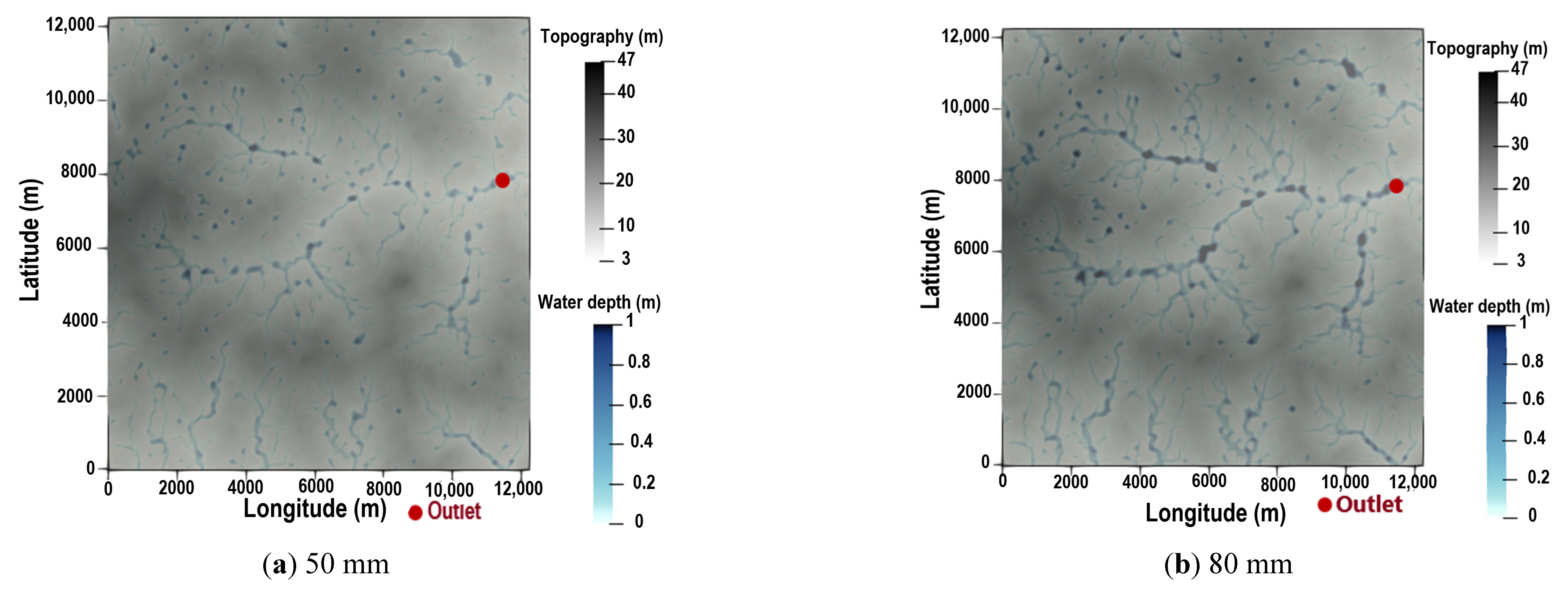
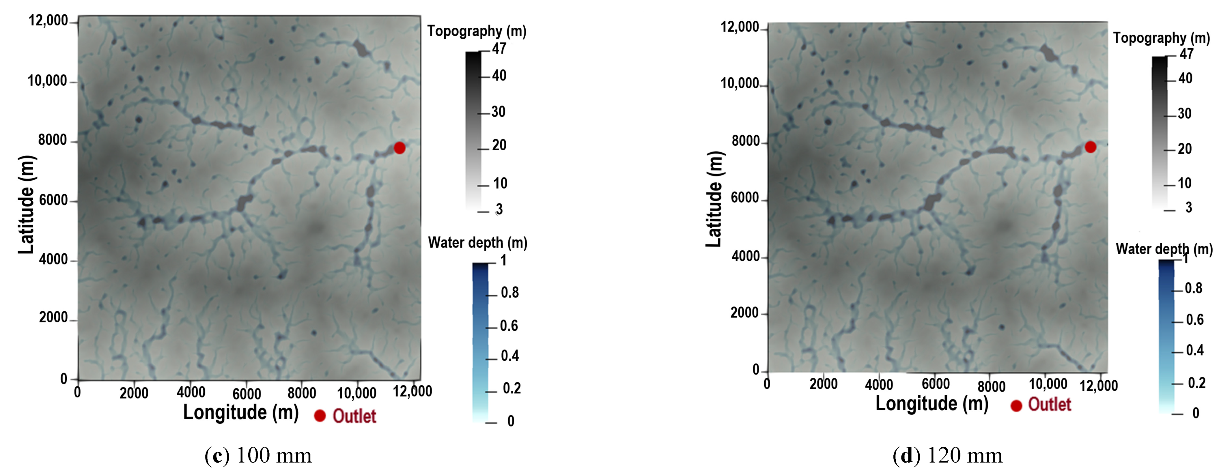
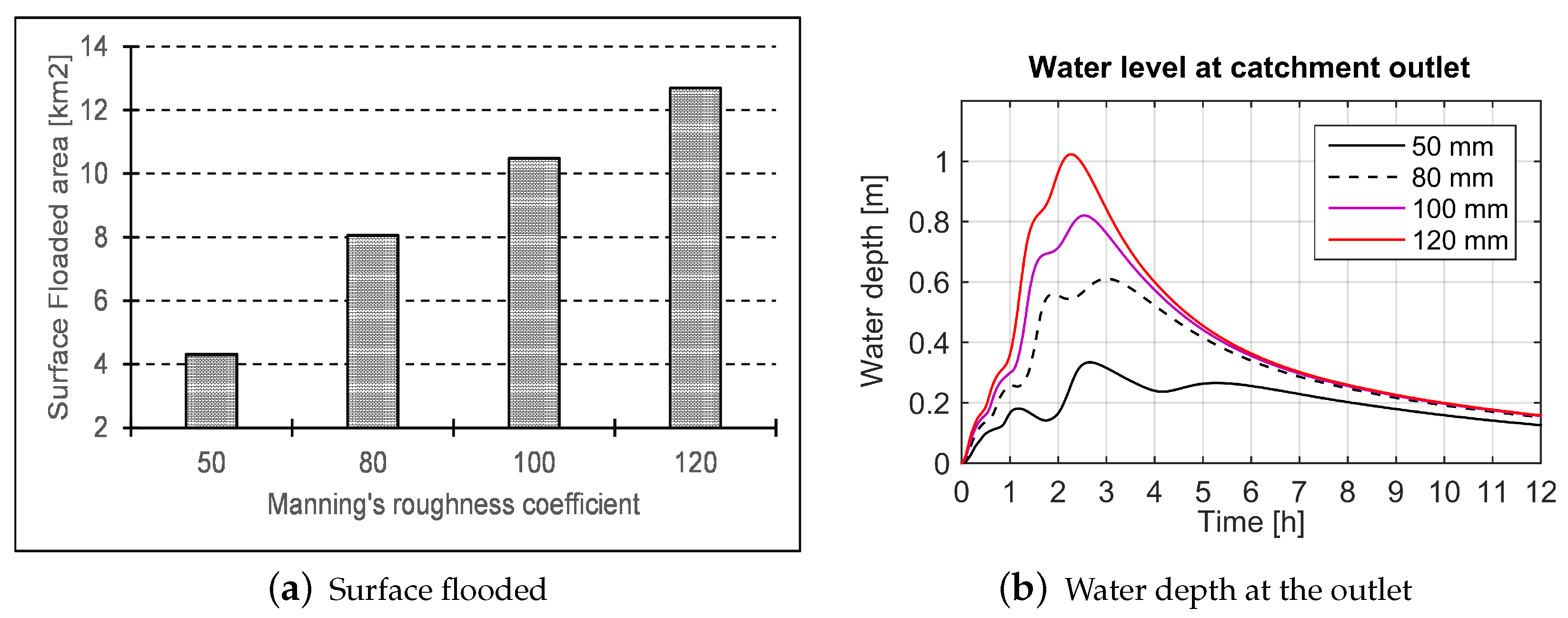
The effect of increasing rainfall intensity on water depth in the watershed is shown in Figure 4 and Figure 5. It can be observed in Figure 4 that the extent of flooded areas increases with an increase in rainfall intensity. Figure 5a indicates that the areas flooded under the four synthetic rainfall intensities varies between 4.3 km 2 and 12.7 km 2 when considering depths exceeding 0.25 m. The surface flooded is not proportional to the rainfall intensity. In fact, the flooded area for the 50 mm synthetic rainfall is 4.3 km 2 , but by multiplying the rainfall intensity by 2 (100 mm), the surface flooded is more than twice 4.3 km 2 (10.5 km 2 ). A similar result is observed at the outlet of the watershed, where the highest water depth (1.1 m) obtained corresponds to the largest rainfall intensity (120 mm) (Figure 5b). The peaks of simulated hydrographs appear between 2 and 3 h, with values varying between 0.32 m for the lowest rainfall (50 mm) and 1.05 m for the highest (120 mm).

4.1.2. Sensitivity Analysis to Manning’s Coefficient

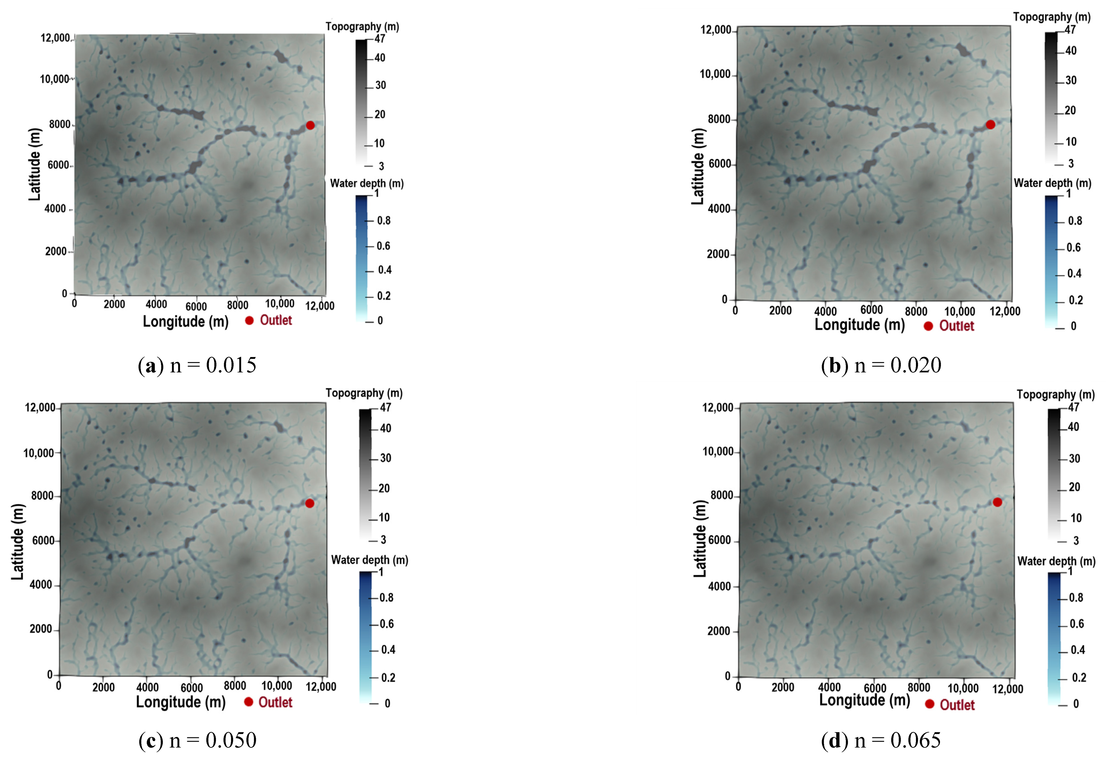
The effect of a roughness coefficient change or different types of land cover is shown in Figure 6 and Figure 7. It can be observed (Figure 6 and Figure 7a) that there was a slight difference between the extent of flooding for urban (n = 0.015) and bare (n = 0.02) land-cover types. An important gap is observed between cultivated (n = 0.050) and vegetated (n = 0.065) land cover for the same rainfall intensity (120 mm) when considering flow depths exceeding 0.25 m. For this scenario, the shape of hydrographs (Figure 7b) is almost similar in the first hour for all simulations. Then a slight shift appears between the peaks for urban and bare soil conditions, while an important gap was realized between cultivated and vegetated land cover.

4.1.3. Sensitivity Analysis to Imperviousness Due to Urbanization

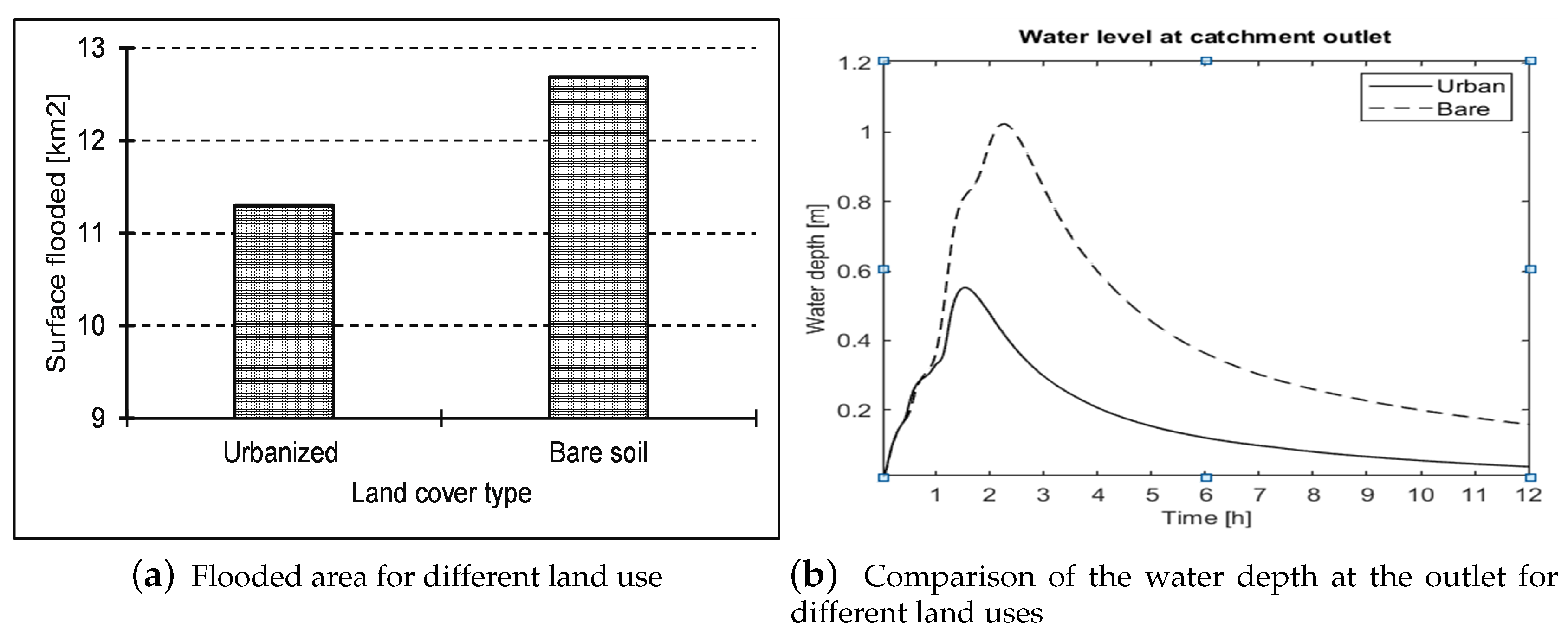
Two simulations were carried out to compare the effects of urbanization on flooding in the watershed. Flood extents for both land-use types (urban and bare soil) are presented in Figure 8. Figure 9a presents the cumulative surface flooded over the watershed and flow depth at the outlet for different land uses. It can be observed that water flows between house blocks (Figure 8a) and follows a natural topography slope in Figure 8b. In urbanized surface conditions, the hydrograph peak (Figure 9b) is observe after 2 h, with a peak depth of 0.57 m, and 3 h for the case of bare soil. The peak depth is more important (1 m) in bare soil conditions compare to the urban surface case.

4.2. Observed Events Simulation

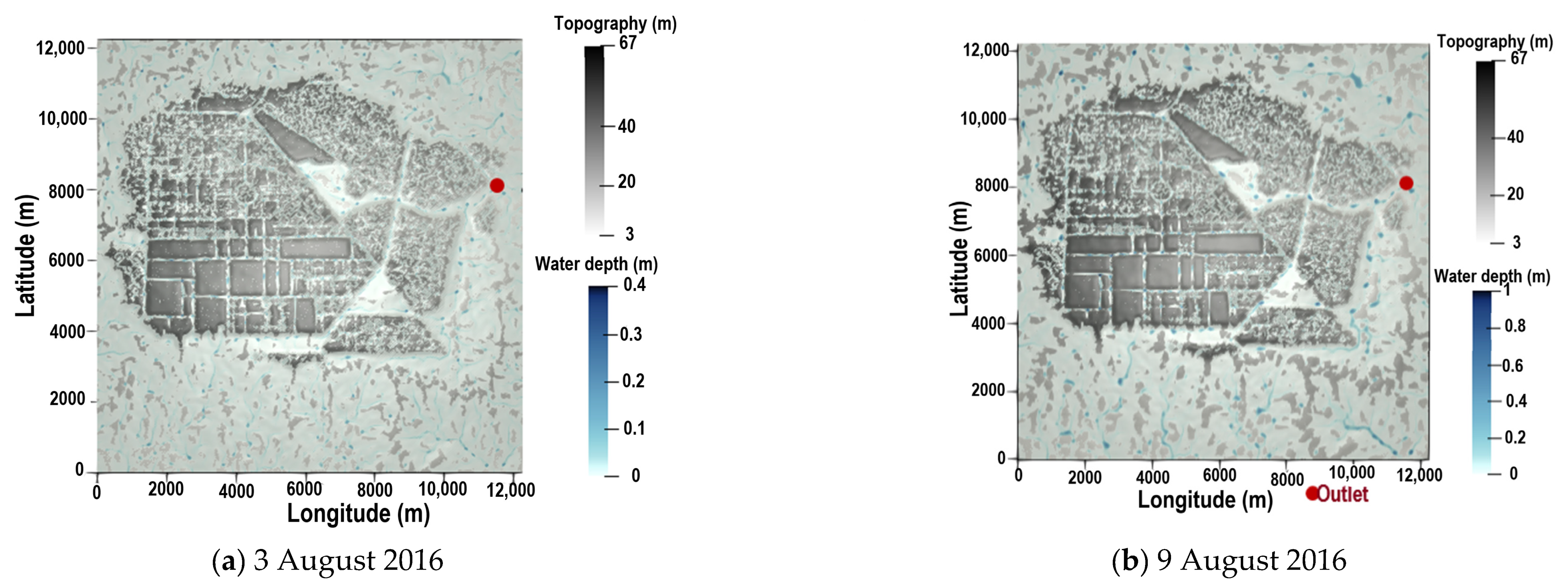
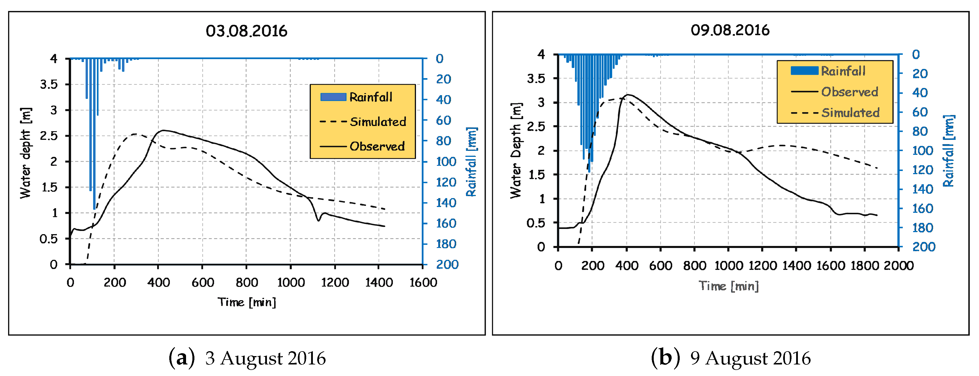
Burkina Faso is frequently hit by tropical heavy rainfall events that cause damage in urban cities such in Ouagadougou. In this study, two monitored rainfall events in 2016 (August 3 and 9) were used for the simulation of real events. Flood maps for both events are shown in Figure 10. Observed and simulated hydrographs at the outlet of the watershed are presented in Figure 11. Simulated water depth for both events showed good agreement with observed data at the respective NSE values of 0.61 and 0.69, showing that the developed model reproduces observed data with acceptable quality.

4.3. Discussion

This paper was devoted to the development of a 2D shallow water model for urban inundation extent using numerical simulation in Ouagadougou. The developed model’s robustness was tested and some real cases simulated. In this study, the developed model parameters (Manning’s roughness coefficient, Horton infiltration model parameters) were collected from the literature due to the difficulties in determining them with accuracy. Topographic data was also constructed from coarse resolution (30 m) satellite information. It was therefore then necessary to assess the model for construction robustness or sensitivity to changes in the selected parameters [38,54]. Sensitivity to rainfall intensity (main input) was first tested through flood spatial extent and water level at the outlet of the catchment due to the considerable spatial variation of rainfall intensity in tropical regions [13,14]. The simulations showed that the more rainfall intensity increases, the greater the extent of flooding, and consequently resulting in an increase in water depth at the outlet. This finding corroborates the results obtained by Laouacheria et al. [57], where the impact of the designed rainfall was investigated using hydraulic tools based on the complete Saint-Venant equations within the Storm Water Management Model (SWMM).
The test of model sensitivity to Manning’s coefficient was carried out by using different values of Manning’s friction coefficient (different land cover) and a unique rainfall intensity for all simulations (120 mm). According to Descroix et al. [25], the rapid land-cover change over the few decades may explain the high frequency [14,26] of floods in most Sahelian regions of West Africa. Increasing values of n were been considered at 0.150, 0.020, 0.050 and 0.065, which correspond, respectively, to urban, bare, cultivated, and vegetated land cover. Simulation results demonstrate a weak impact of increasing n values on flood extent (Figure 6) but an important shift in the time of the water depth peaks. It is then well established that the sensitivity of the developed model to Manning’s friction coefficient variation is weak in flood extent but high in flow depth at the outlet. These results are similar to those obtained by Kumar et al. [54], where the increase (+10% and +20%) or decrease (−10% and −20%) of Manning’s roughness coefficient collected from published literature were found to be affecting water depth.
Another important finding this study demonstrates is the fact that water depth at the outlet is almost similar for urban and bare land covers, with high depth as compared to cultivated and vegetated land-cover type (Figure 7b). For the purpose of flood management, the results demonstrate the important impact of vegetating urban cities or to adopting “green cities” for urban planning to help increase infiltration and thus reduce the stagnation of water over a long period of time.
Model sensitivity to actual urban settlement was tested by comparison with the case where the catchment was considered as uniform, bare land cover. Urbanization and settlement was observed to impact flow by reducing the flood extent and increasing the flood peak at the outlet.
Available data concerning two rainfall events and their corresponding water levels observed at the outlet of the basin in 2016 were used for model calibration and validation. For those rainfall events, the lack of information about flood extent constrained us to compare only the simulated and observed water level as a validation process for the developed model. A good relationship between the observed and simulated water level was shown, with NSEs of, respectively, 0.61 and 0.69 for events 1 and 2.

5. Conclusions

This study focused on the development of a 2D numerical model for urban flood modeling in West Africa. The case study considered is a peri-urban area in Ouagadougou (Burkina Faso). The model is based on shallow-water equations. The numerical solutions are obtained from the finite volume by using structured grids. A sensitivity analysis of this model to input data (rainfall intensity) and its parameters (roughness coefficient and infiltration) revealed the capability of the model developed to simulate flow. Increasing rainfall intensities in the bare soil condition result in increasing water depth within the watershed and in the outlet, and an increase of n affected the hydrograph peak more than the spatial extent of flooding. Imperviousness due to urbanization reduced the flood extent and increased water depth at the outlet. Even though the model developed based on the coarse-resolution DEM (30 m) showed some gaps between observed data and simulated values, the capability of the model to simulate flow over an urban drainage network was demonstrated. The precision of model simulation may depend on DEM accuracy and field soil characteristics but also relies on hydrologic and hydraulic model structure. Even though this model in construction necessitates more improvement (for instance, taking into account drainage network characteristics and testing in various other conditions), this tool may be of great interest for decision makers (urban planners, flood-impact managers, etc.) in Burkina Faso in general, and particularly in Ouagadougou, as it allows the production of maps of maximum water level and flood extent, which is indispensable for effective flood management. This study lays out two important knowledge gaps recommended for further studies:
  • Flood spatial extent has not been validated because of the lack of field data for that process, and thus, high-resolution aerial photographic data of flood extent for flood map validation deserve to be investigated;
  • Sensitivity analysis to digital elevation model resolution for topographic input generation needs to be carried out with a high resolution of 1 m or less to improve accuracy.

Author Contributions

Conceptualization, methodology, and validation, G.C., B.L., F.T., and L.A.M.; resources and data curation, G.C. and B.L.; software, formal analysis, and investigation, G.C., B.L.; writing—original draft preparation, G.C., B.L.; writing—review and editing G.C., B.L., F.T., L.A.M., and H.K.; supervision, project administration, and funding acquisition, H.K. All authors have read and agreed to the published version of the manuscript.

Funding

This work was supported by the World Bank through the Government of Burkina Faso [Grant IDA No. 5420-BF].

Acknowledgments

The authors would like to thank all people who contributed to this work by reading or giving wise advice.

Conflicts of Interest

The authors declare no conflict of interest.

References

  1. Di Baldassarre, G.; Montanari, A.; Lins, H.; Koutsoyiannis, D.; Brandimarte, L.; Blöschl, G. Flood fatalities in Africa: From diagnosis to mitigation. Geophys. Res. Lett. 2010, 37. [Google Scholar] [CrossRef] [Green Version]
  2. Below, R.; Guha-Sapir, D.; Vos, F.; Ponserre, S. Annual Disaster Statistical Review 2010; Centre for Research on the Epidemiology of Disasters: Brussels, Belgium, 2011. [Google Scholar]
  3. Guha-Sapir, D.; Vos, F.; Below, R.; Ponserre, S. Annual Disaster Statistical Review 2014: The Numbers and Trends; Centre for Research on the Epidemiology of Disasters: Brussels, Belgium, 2015. [Google Scholar]
  4. CRED. The Human Cost of Natural Disasters: A Global Perspective; Centre for Research on the Epidemiology of Disasters: Brussels, Belgium, 2015. [Google Scholar]
  5. Erpicum, S.; Dewals, B.; Archambeau, P.; Detrembleur, S.; Pirotton, M. Detailed 2D numerical modeling for flood extension forecasting. In Proceedings of the 4th International Conference on Fluvial Hydraulics: River Flow 2008, Izmir, Turkey, 3–5 September 2008. [Google Scholar]
  6. Okyere, C.Y.; Yacouba, Y.; Gilgenbach, D. The problem of annual occurrences of floods in Accra: An integration of hydrological, economic and political perspectives. Theor. Empir. Res. Urban Manag. 2013, 8, 45–79. [Google Scholar]
  7. Petrucci, O.; Aceto, L.; Bianchi, C.; Bigot, V.; Brázdil, R.; Pereira, S.; Kahraman, A.; Kılıç, Ö.; Kotroni, V.; Llasat, M.C.; et al. Flood fatalities in Europe, 1980–2018: Variability, features, and lessons to learn. Water 2019, 11, 1682. [Google Scholar] [CrossRef] [Green Version]
  8. OCHA. Niger Situation Report; Technical Report; United Nations Office for the Coordination of Humanitarian Affairs: Geneva, Switzerland, 2019. [Google Scholar]
  9. OCHA. Afrique de l’Ouest Inondations 2009; Technical Report; United Nations Office for the Coordination of Humanitarian Affairs: Geneva, Switzerland, 2009. [Google Scholar]
  10. Meehl, G.A.; Stocker, T.F.; Collins, W.D.; Friedlingstein, P.; Gaye, T.; Gregory, J.M.; Kitoh, A.; Knutti, R.; Murphy, J.M.; Noda, A.; et al. Global Climate Projections; Cambridge University Press: Cambridge, UK, 2007. [Google Scholar]
  11. Collins, M.; Knutti, R.; Arblaster, J.; Dufresne, J.L.; Fichefet, T.; Friedlingstein, P.; Gao, X.; Gutowski, W.J.; Johns, T.; Krinner, G.; et al. Long-term climate change: Projections, commitments and irreversibility. In Climate Change 2013-The Physical Science Basis: Contribution of Working Group I to the Fifth Assessment Report of the Intergovernmental Panel on Climate Change; Cambridge University Press: Cambridge, UK, 2013; pp. 1029–1136. [Google Scholar]
  12. Sylla, M.B.; Nikiema, P.M.; Gibba, P.; Kebe, I.; Klutse, N.A.B. Climate change over West Africa: Recent trends and future projections. In Adaptation to Climate Change and Variability in Rural West Africa; Springer: Berlin/Heidelberg, Germany, 2016; pp. 25–40. [Google Scholar]
  13. Taylor, C.M.; Belušić, D.; Guichard, F.; Parker, D.J.; Vischel, T.; Bock, O.; Harris, P.P.; Janicot, S.; Klein, C.; Panthou, G. Frequency of extreme Sahelian storms tripled since 1982 in satellite observations. Nature 2017, 544, 475. [Google Scholar] [CrossRef] [PubMed] [Green Version]
  14. Wilcox, C.; Vischel, T.; Panthou, G.; Bodian, A.; Blanchet, J.; Descroix, L.; Quantin, G.; Cassé, C.; Tanimoun, B.; Kone, S. Trends in hydrological extremes in the Senegal and Niger Rivers. J. Hydrol. 2018, 566, 531–545. [Google Scholar] [CrossRef]
  15. Klutse, N.A.B.; Ajayi, V.O.; Gbobaniyi, E.O.; Egbebiyi, T.S.; Kouadio, K.; Nkrumah, F.; Quagraine, K.A.; Olusegun, C.; Diasso, U.; Abiodun, B.J.; et al. Potential impact of 1.5 C and 2 C global warming on consecutive dry and wet days over West Africa. Environ. Res. Lett. 2018, 13, 055013. [Google Scholar] [CrossRef]
  16. Masson-Delmotte, V.; Zhai, P.; Pörtner, H.O.; Roberts, D.; Skea, J.; Shukla, P.; Pirani, A.; Moufouma-Okia, W.; Péan, C.; Pidcock, R.; et al. Global Warming of 1.5 OC: An IPCC Special Report on the Impacts of Global Warming of 1.5 °C Above Pre-industrial Levels and Related Global Greenhouse Gas Emission Pathways, in the Context of Strengthening the Global Response to the Threat of Climate Change, Sustainable Development, and Efforts to Eradicate Poverty; World Meteorological Organization: Geneva, Switzerland, 2018. [Google Scholar]
  17. OCHA. The Sahel: Converging Challenges, Compounding Risks—A Region under High Pressure; Technical Report; United Nations Office for the Coordination of Humanitarian Affairs: Geneva, Switzerland, 2016. [Google Scholar]
  18. Shekar, M.; Yazbeck, A.; Hasan, R.; Bakilana, A. Population and Development in the Sahel: Policy Choices to Catalyze a Demographic Dividend; World Bank: Washington, DC, USA, 2016. [Google Scholar]
  19. Bani, S.S.; Yonkeu, S. Risques d’inondation dans la ville de Ouagadougou: Cartographie des zones à risques et mesures de prévention. J. Ouest-Afr. Des Sci. Gest. 2016, 1, 1–18. [Google Scholar]
  20. Aich, V.; Koné, B.; Hattermann, F.; Paton, E. Time series analysis of floods across the Niger River Basin. Water 2016, 8, 165. [Google Scholar] [CrossRef] [Green Version]
  21. Oumarou, H.; Oumarou, A. La Gestion Humanitaire des Inondations dans une Commune de Niamey; International Institute for Environment and Development: London, UK, 2017. [Google Scholar]
  22. Tarhule, A. Damaging rainfall and flooding: The other Sahel hazards. Clim. Chang. 2005, 72, 355–377. [Google Scholar] [CrossRef]
  23. Samimi, C.; Fink, A.H.; Paeth, H. The 2007 flood in the Sahel: Causes, characteristics and its presentation in the media and FEWS NET. Nat. Hazards Earth Syst. Sci. 2012, 12, 313–325. [Google Scholar] [CrossRef] [Green Version]
  24. Tschakert, P.; Sagoe, R.; Ofori-Darko, G.; Codjoe, S.N. Floods in the Sahel: An analysis of anomalies, memory, and anticipatory learning. Clim. Chang. 2010, 103, 471–502. [Google Scholar] [CrossRef]
  25. Descroix, L.; Guichard, F.; Grippa, M.; Lambert, L.; Panthou, G.; Mahé, G.; Gal, L.; Dardel, C.; Quantin, G.; Kergoat, L.; et al. Evolution of surface hydrology in the Sahelo-Sudanian strip: An updated review. Water 2018, 10, 748. [Google Scholar] [CrossRef] [Green Version]
  26. Tazen, F.; Diarra, A.; Kabore, R.F.; Ibrahim, B.; Bologo/Traoré, M.; Traoré, K.; Karambiri, H. Trends in flood events and their relationship to extreme rainfall in an urban area of Sahelian West Africa: The case study of Ouagadougou, Burkina Faso. J. Flood Risk Manag. 2019, 12, e12507. [Google Scholar] [CrossRef] [Green Version]
  27. Schlef, K.E.; Kaboré, L.; Karambiri, H.; Yang, Y.E.; Brown, C.M. Relating perceptions of flood risk and coping ability to mitigation behavior in West Africa: Case study of Burkina Faso. Environ. Sci. Policy 2018, 89, 254–265. [Google Scholar] [CrossRef]
  28. Soma, A.; Claude, W.; Sampana, L. Gestion des Inondations dans les Villes de Ouagadougou et de Bobo-Dioulasso dans un Contexte Urbain—Entre jeux D’Acteurs et Logiques Territoriales; Technical Report; Overseas Development Institute (ODI): London, UK, 2018. [Google Scholar]
  29. Garcıa-Navarro, P.; Brufau, P.; Burguete, J.; Murillo, J. The shallow water equations: An example of hyperbolic system. Monogr. Real Acad. Cienc. Zaragoza 2008, 31, 89–119. [Google Scholar]
  30. Hou, J.; Liang, Q.; Zhang, H.; Hinkelmann, R. An efficient unstructured MUSCL scheme for solving the 2D shallow water equations. Environ. Model. Softw. 2015, 66, 131–152. [Google Scholar] [CrossRef] [Green Version]
  31. Bates, P.D.; De Roo, A. A simple raster-based model for flood inundation simulation. J. Hydrol. 2000, 236, 54–77. [Google Scholar] [CrossRef]
  32. Mignot, E.; Paquier, A.; Haider, S. Modeling floods in a dense urban area using 2D shallow water equations. J. Hydrol. 2006, 327, 186–199. [Google Scholar] [CrossRef] [Green Version]
  33. Paquier, A.; Mignot, E.; Bazin, P.H. From hydraulic modelling to urban flood risk. Procedia Eng. 2015, 115, 37–44. [Google Scholar] [CrossRef]
  34. Abily, M.; Bertrand, N.; Delestre, O.; Gourbesville, P.; Richet, Y.; Duluc, C.M. Global sensitivity analysis with 2d hydraulic codes: Applied protocol and practical tool. La Houille Blanche 2015, 16–22. [Google Scholar] [CrossRef] [Green Version]
  35. Abily, M.; Delestre, O.; Gourbesville, P.; Bertrand, N.; Duluc, C.M.; Richet, Y. Global sensitivity analysis with 2D hydraulic codes: Application on uncertainties related to high-resolution topographic data. In Advances in Hydroinformatics; Springer: Berlin/Heidelberg, Germany, 2016; pp. 301–315. [Google Scholar]
  36. Alcrudo, F. A State of the Art Review on Mathematical Modelling of Flood Propagation; First IMPACT Project Workshop: Wallingford, UK, 2002; Available online: http://www.impact-project.net/cd/papers/print/008_pr_02-05-16_IMPACT_Alcrudo.pdf (accessed on 24 July 2020).
  37. Nkwunonwo, U.; Whitworth, M.; Baily, B. A review of the current status of flood modelling for urban flood risk management in the developing countries. Sci. Afr. 2020, 7, e00269. [Google Scholar] [CrossRef]
  38. Maugeri, A. Capabilities of a Coupled 1D/2D Model for Flood Inundation Simulation; Columbia Water Center: New York, NY, USA, 2012. [Google Scholar]
  39. Fan, Y.; Ao, T.; Yu, H.; Huang, G.; Li, X. A coupled 1D-2D hydrodynamic model for urban flood inundation. Adv. Meteorol. 2017, 2017, 2819308. [Google Scholar] [CrossRef] [Green Version]
  40. Anees, M.T.; Abdullah, K.; Nordin, M.N.M.; Ab Rahman, N.N.N.; Syakir, M.I.; Kadir, M.O.A. One-and Two-Dimensional Hydrological Modelling and Their Uncertainties. Flood Risk Manag. 2017, 11, 221–244. [Google Scholar]
  41. Nanía, L.S.; León, A.S.; García, M.H. Hydrologic-hydraulic model for simulating dual drainage and flooding in urban areas: Application to a catchment in the metropolitan area of Chicago. J. Hydrol. Eng. 2015, 20, 04014071. [Google Scholar] [CrossRef]
  42. Bellos, V.; Tsakiris, G. A hybrid method for flood simulation in small catchments combining hydrodynamic and hydrological techniques. J. Hydrol. 2016, 540, 331–339. [Google Scholar] [CrossRef]
  43. Nguyen, P.; Thorstensen, A.; Sorooshian, S.; Hsu, K.; AghaKouchak, A.; Sanders, B.; Koren, V.; Cui, Z.; Smith, M. A high resolution coupled hydrologic–hydraulic model (HiResFlood-UCI) for flash flood modeling. J. Hydrol. 2016, 541, 401–420. [Google Scholar] [CrossRef] [Green Version]
  44. Audusse, E.; Bouchut, F.; Bristeau, M.O.; Klein, R.; Perthame, B.t. A fast and stable well-balanced scheme with hydrostatic reconstruction for shallow water flows. SIAM J. Sci. Comput. 2004, 25, 2050–2065. [Google Scholar] [CrossRef]
  45. Buffard, T.; Gallouet, T.; Hérard, J.M. Un schéma simple pour les équations de Saint-Venant. C. R. Acad. Des. Sci. Paris Ser. 1998, 326, 385–390. [Google Scholar] [CrossRef]
  46. Fraga, I.; Cea, L.; Puertas, J. Validation of a 1D-2D dual drainage model under unsteady part-full and surcharged sewer conditions. Urban Water J. 2017, 14, 74–84. [Google Scholar] [CrossRef]
  47. Toro, E.F. The HLL and HLLC Riemann solvers. In Riemann Solvers and Numerical Methods for Fluid Dynamics; Springer: Berlin/Heidelberg, Germany, 2009; pp. 315–344. [Google Scholar]
  48. Sanders, B.F.; Bradford, S.F. Network implementation of the two-component pressure approach for transient flow in storm sewers. J. Hydraul. Eng. 2011, 137, 158–172. [Google Scholar] [CrossRef]
  49. Deng, X.; Boivin, P.; Xiao, F. A new formulation for two-wave Riemann solver accurate at contact interfaces. Phys. Fluids 2019, 31, 046102. [Google Scholar] [CrossRef] [Green Version]
  50. Arcement, G.J.; Schneider, V.R. Guide for Selecting Manning’s Roughness Coefficients for Natural Channels and Flood Plains; US Geological Survey: Reston, VA, USA, 1989.
  51. Musy, A.; Higy, C. Hydrologie Appliquée Technical Report. Edition HGA, Bucarest. 1998. Available online: https://hydrologie.org/BIB/manuels/Musy1-HGA.pdf (accessed on 24 July 2020).
  52. Pit, R.; Lantrip, J.; Harrison, R.; Henry, C.L.; Xue, D. Infiltration through Disturbed Urban Soils and Compost-Amended Soil Effects on Runoff Quality and Quantity; National Risk Management Research Laboratory: Duluth, GA, USA, 1999.
  53. Hingray, B.; Picouet, C.; Musy, A. Hydrologie: Tome 2, Une Science Pour l’ingénieur; PPUR Presses Polytechniques: Lausanne, Switzerland, 2009; Volume 21. [Google Scholar]
  54. Kumar, M. Sensitivity analysis of Manning’s roughness coefficient in MIKE 11 model for Mahanadi delta region. Ann. Plant Soil Res. 2019, 21, 62–66. [Google Scholar]
  55. Nash, J.A.J.V. River flow forecasting through conceptual models, I: A discussion of principles. J. Hydrol. 1970, 10, 398–409. [Google Scholar] [CrossRef]
  56. Bellos, V.; Tsakiris, G. Comparing various methods of building representation for 2D flood modelling in built-up areas. Water Resour. Manag. 2015, 29, 379–397. [Google Scholar] [CrossRef]
  57. Laouacheria, F.; Kechida, S.; Chabi, M. Modelling the impact of design rainfall on the urban drainage system by Storm Water Management Model. J. Water Land Dev. 2019, 40, 119–125. [Google Scholar] [CrossRef]
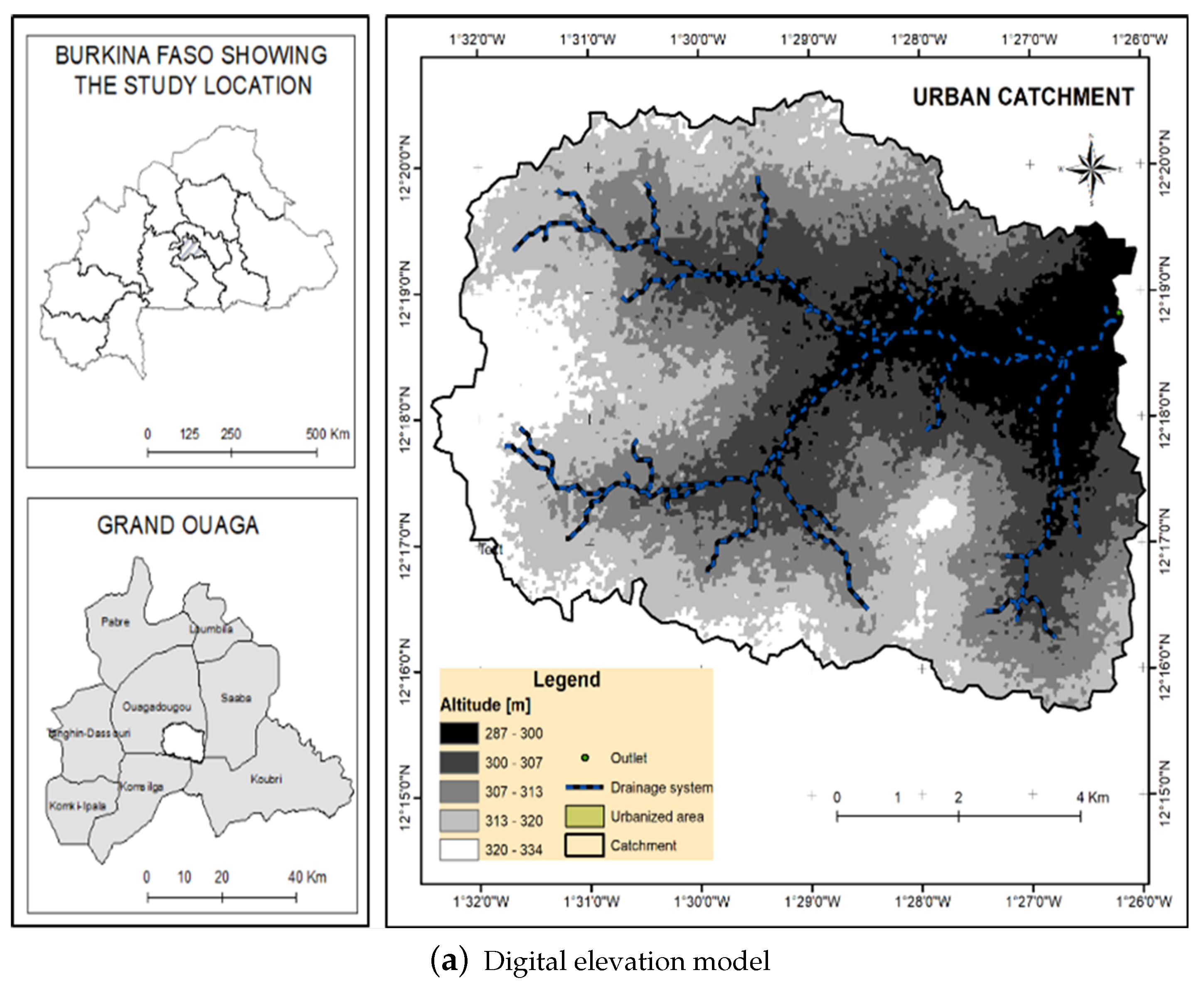
Figure 1. The peri-urban Saaba watershed Digital Elevation Model (a) and urbanized settlement (b).
Water 12 02120 g001aWater 12 02120 g001b
Figure 2. Nodal indexing of elementary cells for the structured mesh.
Water 12 02120 g002
Figure 3. Topographic information with regular grid of 30*30 m resolution.
Water 12 02120 g003
Figure 4. Flood maps for different values of rainfall intensity when the watershed is considered as bare soil.
Water 12 02120 g004aWater 12 02120 g004b
Figure 5. (a) Cumulative flooded surface over the watershed and (b) water depth at the watershed outlet for each rainfall intensity.
Water 12 02120 g005
Figure 6. Flood maps for various values of roughness coefficient.
Water 12 02120 g006
Figure 7. Cumulative flooding of the water level at the outlet for different Manning coefficients.
Water 12 02120 g007
Figure 8. Flood maps after one hour of rain over the watershed for different land-use types.
Water 12 02120 g008
Figure 9. (a) Cumulative area flooded after one hour of uniform synthetic rainfall of 120 mm and (b) evolution of water depth at the outlet after 12 h for different land-cover types.
Water 12 02120 g009
Figure 10. Flood extent for real events.
Water 12 02120 g010
Figure 11. Water depth at the watershed outlet.
Water 12 02120 g011
Table 1. Manning coefficient of the different soil types [50,51].
Land CoverVegetatedBareCultivatedUrban
n [m 1 / 3 / s ]0.0650.0200.0500.015
Table 2. Infiltration parameters of the Horton model for the different soil types [51,52,53].
Land CoverVegetatedBareCultivatedUrban
i 0 [mm/s]* 10 3 0.0290.0050.0210.003
i f [mm/s]* 10 3 0.0970.0170.0690.008
r [1/s]* 10 3 1.3831.3831.3831.383
Table 3. Model parameters used for the sensitivity to rainfall intensity scenario.
Rainfall [mm/hr] i 0 [mm/s]* 10 3 i f [mm/s]* 10 3 r [1/s]* 10 3 n [m 1 / 3 / s ]
500.0050.0171.3830.020
800.0050.0171.3830.020
1000.0050.0171.3830.020
1200.0050.0171.3830.020
Table 4. Model parameters used for the sensitivity to Manning’s coefficient scenario.
Land Covern [m 1 / 3 / s ] i 0 [mm/s]* 10 3 i f [mm/s]* 10 3 r [1/s]* 10 3 Rainfall [mm/hr]
Vegetated0.0650.0290.0971.383120
Bare0.0200.0050.0171.383120
Cultivated0.0500.0210.0691.383120
Urban0.0150.0030.0081.383120
Table 5. Model parameters used for the sensitivity to urbanization scenario.
Land Cover i 0 [mm/s]* 10 3 i f [mm/s]* 10 3 r [1/s]* 10 3 n [m 1 / 3 / s ]Rainfall [mm/hr]
Bare0.0050.0171.3830.02120
Urbanized0.0030.0081.3830.015120