Abstract
Flash flooding is a phenomenon characterized by multiple variables. Few studies have focused on the extracted variables involved in flash flood risk and the joint probability distribution of the extracted variables. In this paper, a novel methodology that integrates the Apriori algorithm and copula function is presented and used for a flood risk analysis of Arizona in the United States. Due to the various rainfall indices affecting the flash flood risk, when performing the Apriori algorithm, the accumulated 3-h rainfall and accumulated 6-h rainfall were extracted as the most fitting rainfall indices. After comparing the performance of copulas, the Frank copula was found to exhibit the best fit for the flash flood hazard; thus, it was used for a bivariate joint probability analysis. The bivariate joint distribution functions of P–Q, PA–Q, PB–Q, and D–Q were established, and the results showed an increasing trend of flash flood risk with increases in the rainfall indices and peak flow; however, the risk displayed the least significant relation with the duration of the flash flood. These results are expected to be useful for risk analysis and decision making regarding flash floods.
1. Introduction
A flash flood is defined as an intense rainfall event or release of water that lasts for minutes to a few hours [1]. Over the last few decades, flash flood events have had devastating impacts on lives and infrastructure, and many flash flood deaths have occurred worldwide. Flash flooding has a complex disaster-causing mechanism. It is caused by a combination of natural and anthropogenic factors [2] including rainfall, topography, watershed, soil, land use, and anthropological activities. Among these factors, rainfall is the major driving force and the most important cause, influencing the magnitude of a flash flood event directly [3]. Intergovernmental Panel on Climate Change (IPCC) has reported that the continued warming situation is expected due to the increase of heavy rainfalls associated with tropical cyclones in some areas, thereby contributing to an increase in flood risks [4]. Many researchers have also implied that the increasing tendency in extreme rainfall activities including severity, duration, and frequency could contribute to the increasing frequency and risk of flash floods in some tropical and subtropical regions [5,6,7]. For example, a study conducted by Billi et.al showed that compared with other factors, the increase in extreme rainfall is likely to play a more important role in the increased frequency of flash floods in Dire Dawa, Ethiopia [8]. Similarly, excluding some regions from central India, an increased flash flood risk accompanied by an increasing trend of extreme rainfall has been found, which is probably caused by climate change [9].
To understand how flood risk varies in different combinations of conditions, some approaches and theories have been developed to derive the quantitative flood risk and construct flood risk maps in recent years. Such methods include the hydrological-hydraulic modeling method [10,11,12,13], the multi-criteria decision method [14,15,16], and the probabilistic analysis method [17,18]. Due to the non-stationarity of flood series, flood frequency analysis is becoming more and more important for flood control and water resource management. With the increasing availability of hydrological monitoring datasets and historical flood datasets, a large flood hazard database could be constructed. Simple statistical methods and probability analysis have been widely used, and numerous studies suggest that they perform well for flash flood forecasting and flood mitigation policy decision-making [19,20,21]. However, the flash flood hazard is regarded as a random process associated with multivariate dependences, so multiple probability models have been used to make these analyses more reliable [22]. Copula functions, one of the probability analysis methods that can be used to model random multivariates and their dependences, are widely used in many study fields. In hydrological drought analysis, as drought events are associated with streamflow, groundwater, soil moisture, and other hydrological processes, the joint distributions of droughts are determined with copula functions [23,24,25,26]. In rainfall and flood analysis, frequency analysis between flood characteristics including peak volume, duration, and rainfall amount is carried out with bivariate copulas [27,28,29,30]. In recent years, copula functions have also been applied to determine the relationships between rainfall and storm tides [31], between floods and droughts [32], and for other multi-variable problems. Previous research has indicated that copula functions perform well in capturing joint behaviors of multiple variables.
Previously, the selection of natural environment indices was the prime task in the probability analysis of flood risk. Rainfall is considered to be an indispensable disaster-triggering factor of flash flood hazard. The selection of rainfall indices directly determines the accuracy in assessing the flash flooding risk. There are many rainfall indices of different durations; however, it is unknown which is the best indicator to assess the hazard accurately and effectively. Furthermore, antecedent rainfall preceding the flood occurrence would result in changes in antecedent soil moisture, which remains to be further investigated [33,34,35,36,37,38]. In preceding studies, the criteria used to select specific rainfall indices varied. For example, Abuzied et al. [39] used the maximum daily rainfall to evaluate the runoff behavior when creating flash flood susceptibility maps in areas characterized by rugged mountainous topography and high relief. Raynaud et al. [40] found that 72 h of rainfall accumulation was a more suitable predictor of flash flooding based on the performance evaluation of EPIC (European Precipitation Index based on Climatology). Youssef et al. [2] utilized the maximal 24-h precipitation over 25 years, 50 years, 100 years, and 200 years as a third dataset to analyze the catastrophic flash flooding events in Jeddah. Moreover, 6-h precipitation data from a flood event were input into the proposed simulation model to assess the flash flooding risk in the upper Teesta River basin [41]. Based on the daily precipitation, the 1-min precipitation, 1-h maximum precipitation, and 12-h maximum precipitation, the characteristics of heavy rainfall were analyzed in flash floods of Aichi Prefecture [42]. Additionally, to explore the changing trends of extreme rainfall events in an area characterized by increasingly strong urbanization, Palermo in Sicily, Italy, a series of maximum rainfall with a fixed duration including 1 h, 3 h, 6 h, 12 h, and 24 h were analyzed by Aronica et al. [43]. The selection of rainfall indices in previous research has mainly depended on experience or literature and was limited by the precipitation datasets; thus, subjectivity and arbitrariness may exist.
Given the above concerns, the current study proposes a multivariate analysis method for assessing the flash flooding risk. The motivation of this study is to determine the rainfall index of flood hazards by using the Apriori algorithm, which is a more objective method for risk index selection; another motivation is to propose a procedure for combined occurrence probability based on selected flooding variates, therefore, the bivariate joint distributions of flooding variates are determined by using the Frank copulas. The results of this study are expected to benefit risk managers and water authorities to better anticipate the potential variates of flash flood hazards, and better cope with the flooding risk by considering the joint effects of multiple variates.
The rest of this paper is organized as follows. Section 2 describes the study area and datasets used; Section 3 gives a description of the methodology used for this study including the Apriori algorithm and the copula function model; Section 4 presents the major results and provides a discussion; and Section 5 presents the conclusions of this work.
2. Study Area
As a demonstration, Arizona State on the Colorado River basin, which has experienced devastating and deadly flash flooding in previous years, was taken as the study region [44]. The Colorado River basin is one of the most highly engineered watersheds in the world. The basin goes through seven states in the United States, and Arizona is one of the states located in the arid area [45]. The Colorado River is located in the northwest of Arizona State, and the Rocky Mountains are at the southeast of Arizona State. Flash flooding is a risk in this study region, and a severe challenge is being faced in flash flood management in this arid area. According to the United States Geological Survey (USGS), there are 134 streamgage stations in the study area (Figure 1). A total of 2066 flooding events recorded in the period from 2008 to 2017 were used in this study, and the peak flow data were obtained from the USGS, while the rainfall datasets were the hourly rainfall data from the NLDAS-2. Besides the role of rapid rainfall in flood hazard, antecedent cumulative rainfall could also contribute to the occurrence of flash floods. Based on a literature review and collection of rainfall indicators, six rainfall magnitude indicators with different durations during these flooding events were calculated in this study, namely, the maximum 1-h rainfall (P), accumulated 3-h rainfall (PA), accumulated 6-h rainfall (PB), accumulated 12-h rainfall (PC), accumulated 24-h rainfall (PD), and accumulated 72-h rainfall (PE), respectively, and have been the most widely used in previous studies [5,7,39,40,41,42,43,46]. Further exploration was carried out in this study to select the best ones for use in flash flood analysis. Simultaneously, four temporal indicators were taken into consideration in this study including the flooding year (YR), flooding month (MH), flooding days (FT), and flood duration (D) to analyze the temporal distribution of the flash floods in the study area.
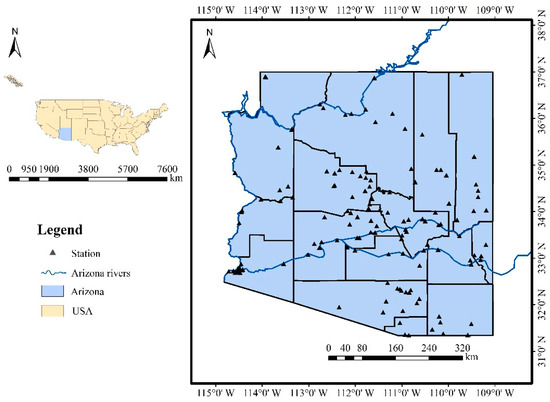
Figure 1.
Map of the study area.
3. Methods
In this study, a multivariate analysis method is proposed that integrates the Apriori algorithm and copula function. First, data pre-processing was conducted by K-means clustering, and the various rainfall indices were classified into several conditions; then, the Apriori algorithm was applied to extract the rainfall index for the risk analysis of flash floods; by using the copula function, bivariate joint distribution of flood variates were determined, and the probability distributions and probability isolines were analyzed. The flow-chart of the methodology in this study is shown in Figure 2.
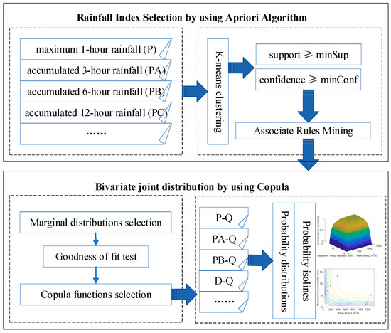
Figure 2.
Flow-chart of the methodology.
3.1. Apriori Algorithm
Association rules (AR), one of the instrumental technologies used in data mining, are used to discover correlations and appear as regularities among items in the database [47,48]. Since association rule algorithms can only process discrete data, it is necessary to discretize the collected continuous data first. The K-means clustering approach, a method that is widely used to cluster large datasets because of its simplicity, efficiency, and easy implementation, has led to its popular application for partitioning data in a variety of fields [49,50,51]. It was applied in the present study to tackle the requirement of data discretization. Its objective is to allocate a mass of objects into k clusters where each object belongs to the cluster with the nearest mean, thereby minimizing the difference within the clusters.
There are some basic definitions and concepts used in the mining procedure of association rules. Let represent a set of all items (i) and a set of transactions (t), respectively. A rule is defined as ‘’, where . X is the antecedent and is the consequent. This rule means that if ‘X occurred in D’, then there is a trend of ‘ occurred in D’.
Additionally, there are two best-known parameters that are used to judge the rules [52]: ‘Support’ and ‘Confidence’. The former is used to measure the frequency of the item or the items in the rule that occur together, and the latter is used to measure how often the rule has been found to be true. These are defined by the formulas below, where |∙| represents the number of elements in the set.
support (X) = |{X⊆D}|/|{D}|
support (X⇒Y) = |{X∪Y⊆D}|/|{D}|
confidence (X⇒Y) = |{X∪Y⊆D}|/|{X⊆D}|
Moreover, the minimum support threshold (minSup) and minimum confidence threshold (minConf) can be set to satisfy the demands of users. If support () ≥ minSup, is a frequent item set; if support () ≥ minSup and confidence () ≥ minConf, then is a strong association rule.
Lift is employed to gauge the correlation between the components in a rule. When the lift is larger than 1, has a positive correlation with ; when the lift is less than 1, has a negative correlation with :
lift (X⇒Y) = {X∪Y⊆D}/{X⊆D}/{Y⊆D}/{D}.
The Apriori algorithm was developed by Agrawal and Srikant [53] and has become a classical technique for discovering frequent item sets. It uses a bottom-up iterative method, improving the computing efficiency because of its connection steps and pruning steps. The Apriori algorithm usually involves two steps: in the first step, given minSup, all of the frequent items in the database are filtered out; in the second step, given minConf, all of the strong association rules are mined based on the frequent item results.
3.2. Copula Function
Due to the dependent variables in the hydrological problems, copulas are functions that are used to facilitate the modeling of the dependency between two or more variables, and they allow the flexibility of choosing the marginal distributions of the individual variables [54]. Copulas were first introduced in 1959. Sklar’s theorem states that, suppose there are random variables X1, X2, X3, …, Xn, the distribution of marginals is F1(X1), F2(X2), F3(X3), …, Fn(Xn), respectively, and the joint behavior of these variables can be characterized by the copula function, C:
where F is the joint cumulative distribution function (CDF) of random variables; Fi(Xi) is the continuous distribution of marginals; ; and i = 1, 2, …, n.
The Elliptic copula family and the Archimedean copula family have been widely used. As a demonstration, the Elliptic copula family, with the Gaussian copula and t-copula members, and the Archimedean copula family including the Gumbel copula, Clayton copula, and Frank copula were selected for use in this study. The cumulative distribution expressions are shown in Table 1, let u, v be random variables; Φ is known as a generator function of the copula and Φ−1 is the inverse of Φ; θ is the copula parameter. More details on the theoretical properties of various copulas can also be found in [55].

Table 1.
Cumulative distributions of copulas.
For the goodness of fit test, this study utilized the Square Euclidean distance (D2) and ordinary least square (OLS) to assess the fitting quality between theoretical and empirical distributions of samples and select the optimal copula. The goodness of fit is believed to be better when a smaller D2 or OLS value is obtained. The D2 and OLS are specifically written as follows:
where is the empirical copula function.
where is the empirical distribution of the joint probability of the i-parameter; is the theoretical distribution of the joint probability of the i-parameter; and n is the number of parameters.
4. Results and Discussion
4.1. Association Rules
4.1.1. Classification Using K-Means Cluster
Four rainfall temporal indices, YR, MH, FT, and D were divided into four chronological groups, as displayed in Table 2. The continuous indices P, PA, PB, PC, PD, and PE were classified into four groups by using K-means clustering analysis, and in order of magnitude, these four groups were considered to represent small, moderate, large, and heavy rainfall, respectively. This study regarded the flooding return period as the classified judgement of the flood hazard magnitude. Similarly, four levels of flood hazard were regarded: small-hazard, moderate-hazard, large-hazard, and heavy-hazard. The classification results of the flood hazard and rainfall indices are shown in Table 2, and the proportions of the four levels in the rainfall indices are shown in Figure 3. The results show that most historical floods occurred within two days, with precipitation lasting no more than 24 h. Moreover, almost 80% of historical floods had small and moderate rainfall of different durations, and floods usually hit Arizona in the summer (from April to July) and winter (from January to March). It is noticeable that the frequency of flooding events over the period from 2008 to 2017 was lower than that over the period from 1998 to 2007.
Table 2.
Classification results for the flood hazard and rainfall indices.
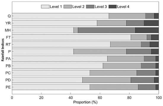
Figure 3.
Proportion of the four levels in the rainfall indices.
4.1.2. Associate Rules Mining Using the Apriori Algorithm
The Apriori algorithm is used in association rule mining to explore relationships among all indicators and identify the most suitable rainfall indices that have the strongest associations with flash flooding hazard in the study area.
First, the Apriori algorithm was used to explore frequent item sets. Based on the historical flood database of Arizona State over the period from 1998 to 2017, this study found that the mining results were satisfactory when minSup = 0.4 was used. As listed in Table 3, 30 frequent item sets were found in total, and the support indicates the frequency of flooding events of Arizona State. The results show that the top two frequent item sets of single indices were a maximum 3-h rainfall level of less than 2.5 mm (PA1) and a maximum 6-h rainfall level of less than 5 mm (PB1), accounting for 66.0% and 62.5%, respectively. Furthermore, ‘PA1, PB1’ accounted for the largest percentage among multiple frequent item sets with 56.3%, which indicates that PA1 and PB1 usually occur together in the historical flash flood database. For temporal indicators, ‘FT1’ accounted for the largest percentage of 80.8%, which means that most of the historical flash floods occurred in the study area for one or two days only. The top three frequent item sets of multiple indicators were ‘PA1, FT1’, ‘PB1, FT1’, and ‘PA1, PB1, FT1’, which further show that these three items appear frequently in the database.
Table 3.
Frequent item sets for the rainfall indices.
Second, the Apriori algorithm was further applied to investigate strong association rules in the database, and by setting minSup = 0.2 and minConf = 0.56, 78 strong association rules were generated. Figure 4 presents the distribution of these strong association rules, a scatter point in a color close to blue means that the lift of the rule was less than 1, namely, the components in the rule had a negative correlation, and vice versa. Table 4 only displays 31 rules with the support of more than 0.24 to get a better understanding of some specific rules. In terms of the strong association rules of a single rainfall magnitude index, ‘Rule 1: PA1->Q1’ (42.7%) and ‘Rule 2: PB1->Q1’ (39.6%) had the top two support values, far more than the third support (31.9%). Taking ‘Rule 1’ as an example, a support level of 42.7% and a confidence level of 64.7% was found, which implies a strong association between PA1 and Q1. The proportion of the flood events containing PA1 and Q1 was 42.7%, and 64.7% of the flood events containing PA1 also contained Q1. Furthermore, with respect to the rules of multiple rainfall magnitude indices, with a support level of 35.6% and a confidence level of 65.3%, ‘Rule 8: PA1, PB1->Q1’ also had a large amount of support and confidence. Regarding the temporal indices, the support values of ‘Rule 24: PA1, FT1->Q1’ and ‘Rule 25: PB1, FT1->Q1’ had the top two values, which were more than 32%. This again suggests that a high frequency of small-hazard flash flooding occurs with a small magnitude of 3-h and 6-h rainfalls. In other words, it can be concluded that the accumulated 3-h (PA) and 6-h rainfall (PB) values are the most fitting rainfall indicators to assess the flash flood hazard compared with other rainfall magnitude indices.
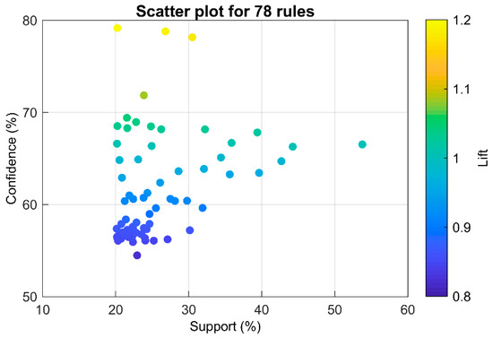
Figure 4.
Distribution of association rules.
Table 4.
Strong association rules mined by association rules.
4.2. Probability Distribution Analysis
Assuming that the peak flow (Q, m3/s), duration (D, h), maximum 1-h rainfall (P, mm), accumulated 3-h rainfall (PA, mm), and accumulated 6-h rainfall (PB, mm) of flash flood events were continuous random variables, the marginal distributions of flood variables were analyzed, and the bivariate joint distribution functions of P–Q, PA–Q, PB–Q, and D–Q were conducted.
Taking P–Q as an example, the frequency histograms are shown in Figure 5. The results show that the unsymmetrical peak flow was concentrated at less than 200 m3/s and the maximum 1-h rainfall was distributed less than 5 mm. The variables do not obey a normal distribution, thus, the parametric methods (i.e., Gamma distribution, Weibull distribution) were evaluated using the OLS and AIC criteria. The results are present in Table 5, which provides a comparison for justifying the best fitting marginal distributions. Due to the lower OLS and AIC value, Gramma distribution was chosen for marginal distribution of Q and P in this study.
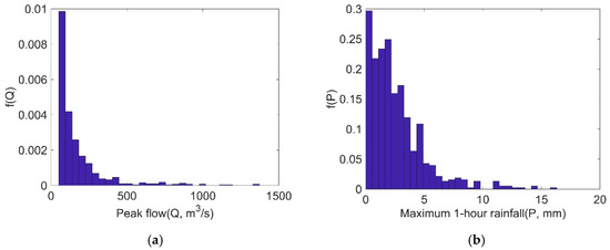
Figure 5.
Frequency histograms. (a) Peak flow; (b) Maximum 1-h rainfall.
Table 5.
Performance of parametric methods for fitting marginal distributions of various floods.
Among the various copula function families mentioned in Section 3.2, the Gaussian copula, t-copula, Gumbel copula, Clayton copula, and Frank copula were used to determine the joint distribution of P–Q. Furthermore, m-copula, based on the Clayton copula, Gumbel copula, and Frank copula was developed. The formulation is written as follows [56]:
where, θ1, θ2, and θ3 are the parameters of the Clayton copula, Gumbel copula, and Frank copula, respectively, and α1 + α2 + α3 = 1.
m-Copula = α1Clayton(θ1) + α2Gumbel(θ2) + α3Frank(θ3)
The probability density distributions of various copula functions were estimated, as shown in Figure 6. The parameters of different copula function are as follows: ρ(Gaussian) = ; ρ(t) = , k = 11.6; θ(Gumbel) = 1.0378; θ(Clayton) = 0.1518; θ(Frank) = 0.4275; in m-Copula, α1 = 0.2407, α2 = 0.4370, α3 = 0.3223, θ1 = 0.7818, θ2 = 1.0000, θ3 = 0.4275.
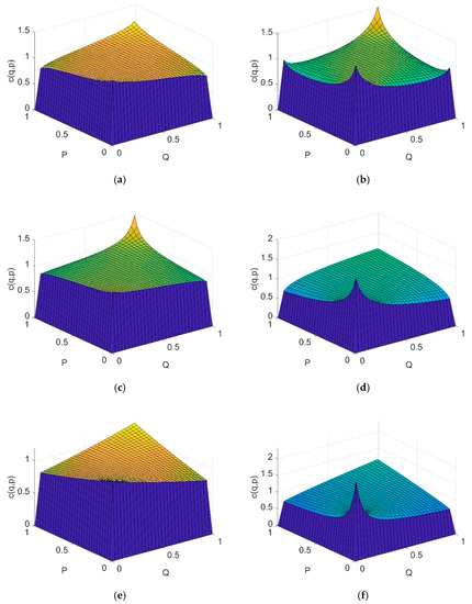
Figure 6.
Probability density distribution. (a) Gaussian copula; (b) t-copula; (c) Gumbel copula; (d) Clayton copula; (e) Frank copula; (f) m-copula.
The performance of each copula function was evaluated by the Square Euclidean distance (D2) and ordinary least square (OLS), as shown in Table 6. The results indicate that the six copula functions all passed the D2 test and OLS test, and the smallest value was shown with the Frank function. Therefore, the Frank copula was adopted for further analysis of flood characteristics, and the bivariate joint probability distributions of P–Q were estimated. The results are shown in Figure 6. The combined probability of the maximum 1-h rainfall and peak flow can be found in Figure 7. With an increase in P, the combined occurrence probability of flood hazard increases correspondingly; with an increase in Q, the combined occurrence probability of flood hazard also increases. For example, when the maximum 1-h rainfall is 5 mm and the peak flow is 200 m3/s, the flood occurrence probability is 0.65; when the maximum 1-h rainfall increases to 10 mm, the flood occurrence probability increases to 0.72, correspondingly; when the maximum 1-h rainfall is 5 mm and the peak flow is 500 m3/s, the occurrence probability of floods is 0.84.
Table 6.
Evaluation results of copula functions.
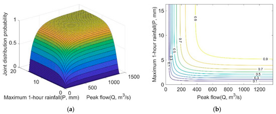
Figure 7.
Probability distribution of P–Q using Frank (a) bivariate joint probability distributions; (b) probability isolines.
Based on the above analysis, the bivariate joint probability distributions of D–Q, PA–Q, and PB–Q were also determined. Table 7 presents the statistical parameters of samples in different bivariate joint probability distributions. Suppose x1, x2, …, xn are the samples of flood various, EX is defined as the mean value of samples; Cv is the variation coefficient, which is used to measure the relative dispersion; and Cs is the deviation coefficient, which is used to describe the asymmetry on the sides of mean value.
where σ is the mean square error.
Table 7.
Statistical parameters.
Table 8 presents the values of the estimated parameter θ of the Frank copula in different bivariate joint probability distributions, and bivariate joint probability distributions of PA–Q, PB–Q, and D–Q are shown in Figure 8. The results show that the bivariate joint probability increased as the amount of rainfall increased, and the contour curves displayed similar shapes. The combined probability of the rainfall index and peak flow can be found in Figure 8a,b. For example, when the maximum 3-h rainfall is 6 mm and the peak flow is 200 m3/s, the flood occurrence probability will be 0.60; when the maximum 3-h rainfall is 5 mm and the peak flow is 400 m3/s, the flood occurrence probability increases to 0.60. Furthermore, when the maximum 6-h rainfall is 10 mm and the peak flow is 250 m3/s, the flood occurrence probability is 0.65, and when the maximum 6-h rainfall is 5 mm and the peak flow is 300 m3/s, the flood occurrence probability decreases to 0.46. The results also highlight that the combined occurrence probability based on the Frank copula described the relative relation of multiple various, in this way, more objective characteristics of flood hazards were displayed.
Table 8.
Parameter θ of the Frank copula.
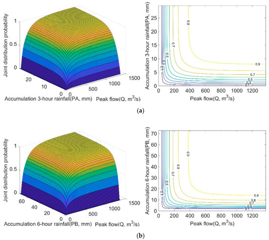
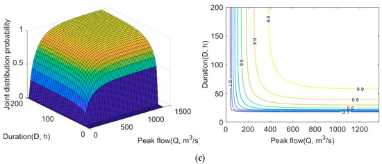
Figure 8.
Bivariate joint probability distributions and probability isolines (a) PA–Q; (b) PB–Q; and (c) D–Q.
For flood duration, as can be seen in Figure 8c, the combined probability of duration and peak flow is generally less than 0.60. The flash flood risk is mostly affected by the peak flow rather than the duration. The results correspond to the characteristics of flash floods that occur suddenly and within a duration of 6 h.
5. Conclusions
Flash flooding is a phenomenon characterized by peak flow, duration, and rainfall indices. In this paper, the rainfall indices were mined by the Apriori algorithm, and the most fitting rainfall indices for flood risk analysis were extracted. Then, the combination probability distributions of flood variables were linked by the copula function, and based on the margination distribution and goodness-of-fit test, the best fit copula model was obtained. The following specific conclusions were made:
- (1)
- Using the Apriori algorithm, accumulated 3-h rainfall and accumulated 6-h rainfall were extracted as the most fitting rainfall indices, and these can be used for the risk analysis of flash floods.
- (2)
- The bivariate joint distributions of flooding properties were determined by using the Frank copula, and then the bivariate joint distribution functions of P–Q, PA–Q, PB–Q, and D–Q were conducted. The increasing flash flooding risk trend was illustrated with increases in rainfall indices and peak flow; however, the risk displayed the least significant relation with the duration of flash floods. These results are expected to be useful for risk analysis and decision making in flash flood assessment.
Author Contributions
Conceptualization, M.Z. and T.J.; Methodology, J.W.; Formal Analysis, M.Z.; Investigation, Z.H.; Data Curation, Z.H.; Writing—Original Draft Preparation, M.Z.; Writing—Review & Editing, T.J., X.C. and Y.H.; Project Administration, X.C. and M.Z. All authors have read and agreed to the published version of the manuscript.
Funding
The research was supported by the National Natural Science Foundation of China (Grant No. U1911204 and Grant No. 51709286), the Guangdong Natural Science Foundation of China (No. 2017A030310065), and the Young Teacher Development Program of Sun Yat-Sen University (Grant No. 19lgpy49).
Acknowledgments
The authors would like to thank the graduate students who worked on data collection.
Conflicts of Interest
The authors declare no conflicts of interest.
References
- Saharia, M.; Kirstetter, P.E.; Vergara, H.; Gourley, J.J.; Hong, Y.; Giroud, M. Mapping Flash Flood Severity in the United States. J. Hydrometeorol. 2017, 18, 397–411. [Google Scholar] [CrossRef]
- Youssef, A.M.; Sefry, S.A.; Pradhan, B.; Alfadail, E.A. Analysis on causes of flash flood in Jeddah city (Kingdom of Saudi Arabia) of 2009 and 2011 using multi-sensor remote sensing data and GIS. Geomat. Nat. Hazards Risk 2015, 7, 1018–1042. [Google Scholar] [CrossRef]
- Sangati, M.; Borga, M.; Rabuffetti, D.; Bechini, R. Influence of rainfall and soil properties spatial aggregation on extreme flash flood response modelling: An evaluation based on the Sesia river basin, North Western Italy. Adv. Water Resour. 2009, 32, 1090–1106. [Google Scholar] [CrossRef]
- IPCC. Managing the Risks of Extreme Events and Disasters to Advance Climate Change Adaptation; Cambridge University Press: Cambridge, UK; New York, NY, USA, 2012. [Google Scholar]
- Groisman, P.Y.; Knight, R.W.; Karl, T.R.; Easterling, D.R.; Sun, B.; Lawrimore, J.H. Contemporary changes of the hydrological cycle over the contiguous United States: Trends derived from in situ observations. J. Hydrometeorol. 2004, 5, 64–85. [Google Scholar] [CrossRef]
- Zhong, M.; Jiang, T.; Li, K.; Lu, Q.; Wang, J.; Zhu, J. Multiple environmental factors analysis of flash flood risk in Upper Hanjiang River, southern China. Environ. Sci. Pollut. Res. 2019, 1–11. [Google Scholar] [CrossRef]
- Ballesteros-Cánovas, J.A.; Czajka, B.; Janecka, K.; Lempa, M.; Kaczka, R.J.; Stoffel, M. Flash floods in the Tatra Mountain streams: Frequency and triggers. Sci. Total Environ. 2015, 511, 639–648. [Google Scholar] [CrossRef] [PubMed]
- Billi, P.; Alemu, Y.T.; Ciampalini, R. Increased frequency of flash floods in Dire Dawa, Ethiopia: Change in rainfall intensity or human impact? Nat. Hazards 2015, 76, 1373–1394. [Google Scholar] [CrossRef]
- Guhathakurta, P.; Sreejith, O.P.; Menon, P.A. Impact of climate change on extreme rainfall events and flood risk in India. J. Earth Syst. Sci. 2011, 120, 359–373. [Google Scholar] [CrossRef]
- Mandal, S.P.; Chakrabarty, A. Flash flood risk assessment for upper Teesta river basin: Using the hydrological modeling system (HEC-HMS) software. Modeling Earth Syst. Environ. 2016, 2, 1–10. [Google Scholar] [CrossRef]
- Nguyen, P.; Thorstensen, A.; Sorooshian, S.; Hsu, K.; AghaKouchak, A.; Sanders, B.; Koren, V.; Cui, Z.; Smith, M. A high resolution coupled hydrologic–hydraulic model (HiResFlood-UCI) for flash flood modeling. J. Hydrol. 2016, 541, 401–420. [Google Scholar] [CrossRef]
- Wu, H.; Adler, R.; Tian, Y.; Gu, G.; Huffman, G. Evaluation of Quantitative Precipitation Estimations through Hydrological Modeling in IFloodS River Basins. J. Hydrometeorol. 2017, 18, 529–553. [Google Scholar] [CrossRef]
- Li, W.; Lin, K.; Zhao, T.; Lan, T.; Chen, X.; Du, H.; Chen, H. Risk assessment and sensitivity analysis of flash floods in ungauged basins using coupled hydrologic and hydrodynamic models. J. Hydrol. 2019, 572, 108–120. [Google Scholar] [CrossRef]
- Shehata, M.; Mizunaga, H. Flash flood risk assessment for Kyushu Island, Japan. Environ. Earth Sci. 2018, 77, 1–20. [Google Scholar] [CrossRef]
- Zhong, M.; Wang, J.; Gao, L.; Lin, K.R.; Hong, Y. Fuzzy risk assessment of flash floods using a cloud-based information diffusion approach. Water Resour. Manag. 2019, 33, 2537–2553. [Google Scholar] [CrossRef]
- Lin, K.; Chen, H.; Xu, C.; Yan, P.; Lan, T.; Liu, Z.; Dong, C. Assessment of flash flood risk based on improved analytic hierarchy process method and integrated maximum likelihood clustering algorithm. J. Hydrol. 2020, 584, 124696. [Google Scholar] [CrossRef]
- Salvadori, G.; Durante, F.; De Michele, C.; Bernardi, M. Hazard Assessment under Multivariate Distributional Change-Points: Guidelines and a Flood Case Study. Water 2018, 10, 751. [Google Scholar] [CrossRef]
- Gu, H.; Yu, Z.; Li, G.; Ju, Q. Nonstationary Multivariate Hydrological Frequency Analysis in the Upper Zhanghe River Basin, China. Water 2018, 10, 772. [Google Scholar] [CrossRef]
- Wang, Z.; Lai, C.; Chen, X.; Yang, B.; Zhao, S.; Bai, X. Flood hazard risk assessment model based on random forest. J. Hydrol. 2015, 527, 1130–1141. [Google Scholar] [CrossRef]
- Alfonso, L.; Mukolwe, M.M.; Di Baldassarre, G. Probabilistic flood maps to support decision-making: Mapping the value of information. Water Resour. Res. 2016, 52, 1026–1043. [Google Scholar] [CrossRef]
- Brandon, P.; David, D. Defining the hundred year flood: A Bayesian approach for using historic data to reduce uncertainty in flood frequency estimates. J. Hydrol. 2016, 540, 1189–1208. [Google Scholar]
- Guerriero, L.; Ruzza, G.; Guadagno, F.M.; Revellino, P. Flood hazard mapping incorporating multiple probability models. J. Hydrol. 2020, 587, 125020. [Google Scholar] [CrossRef]
- Song, S.; Singh, V.P. Frequency analysis of droughts using the Plackett copula and parameter estimation by genetic algorithm. Stoch. Environ. Res. Risk Assess. 2010, 24, 783–805. [Google Scholar] [CrossRef]
- Chen, Y.D.; Zhang, Q.; Xiao, M.; Singh, V.P. Evaluation of risk of hydrological droughts by the trivariate Plackett copula in the East River basin (China). Nat. Hazards 2013, 68, 529–547. [Google Scholar] [CrossRef]
- Tu, X.; Du, Y.; Singh, V.P.; Chen, X.; Zhao, Y.; Ma, M.; Wu, H. Bivariate Design of Hydrological Droughts and Their Alterations under a Changing Environment. J. Hydrol. Eng. 2019, 24, 04019015. [Google Scholar] [CrossRef]
- Vo, Q.; So, J.; Bae, D. An Integrated Framework for Extreme Drought Assessments Using the Natural Drought Index, Copula and Gi * Statistic. Water Resour. Manag. 2020, 34, 1353–1368. [Google Scholar] [CrossRef]
- Kao, S.C.; Govindaraju, R.S. Trivariate statistical analysis of extreme rainfall events via the Plackett family of copulas. Water Resour. Res. 2008, 44, 333–341. [Google Scholar] [CrossRef]
- Zhang, Q.; Li, J.; Singh, V.P.; Xu, C. Copula-based spatiotemporal patterns of precipitation extremes in China. Int. J. Climatol. 2013, 33, 1140–1152. [Google Scholar] [CrossRef]
- Jeong, D.I.; Sushama, L.; Khaliq, M.N.; Roy, R. A copula-based multivariate analysis of Canadian RCM projected changes to flood characteristics for Northeastern Canada. Clim. Dyn. 2014, 42, 2045–2066. [Google Scholar] [CrossRef]
- Abdollahi, S.; Akhoond-Ali, A.; Mirabbasi, R.; Adamowski, J.F. Probabilistic Event Based Rainfall-Runoff Modeling Using Copula Functions. Water Resour. Manag. 2019, 33, 3799–3814. [Google Scholar] [CrossRef]
- Xu, K.; Ma, C.; Lian, J.; Bin, L. Joint probability analysis of extreme precipitation and storm tide in a coastal city under changing environment. PLoS ONE 2014, 9, e109341. [Google Scholar] [CrossRef]
- Tu, X.; Du, X.; Singh, V.P.; Chen, X.; Du, Y.; Li, K. Joint Risk of Interbasin Water Transfer and Impact of the Window size of Sampling low flows under Environmental Change. J. Hydrol. 2017, 554, 1–11. [Google Scholar] [CrossRef]
- Rahardjo, H.; Li, X.; Toll, D.G.; Leong, E.C. The effect of antecedent rainfall on slope stability. Geotech. Geol. Eng. 2001, 19, 371–399. [Google Scholar] [CrossRef]
- Michele, D.C.; Salvadori, G. On the derived flood frequency distribution: Analytical formulation and the influence of antecedent soil moisture condition. J. Hydrol. 2002, 262, 245–258. [Google Scholar] [CrossRef]
- Javelle, P.; Fouchier, C.; Arnaud, P.; Lavabre, J. Flash flood warning at ungauged locations using radar rainfall and antecedent soil moisture estimations. J. Hydrol. 2010, 394, 267–274. [Google Scholar] [CrossRef]
- Grillakis, M.G.; Koutroulis, A.G.; Komma, J.; Tsanis, I.K.; Wagner, W.; Blöschl, G. Initial soil moisture effects on flash flood generation—A comparison between basins of contrasting hydro-climatic conditions. J. Hydrol. 2016, 541, 206–217. [Google Scholar] [CrossRef]
- Tramblay, Y.; Bouvier, C.; Martin, C.; Didon-Lescot, J.F.; Todorovik, D.; Domergue, J.M. Assessment of initial soil moisture conditions for event-based rainfall–runoff modelling. J. Hydrol. 2010, 387, 176–187. [Google Scholar] [CrossRef]
- Zhai, X.; Guo, L.; Liu, R.; Zhang, Y. Rainfall threshold determination for flash flood warning in mountainous catchments with consideration of antecedent soil moisture and rainfall pattern. Nat. Hazards 2018, 94, 605–625. [Google Scholar] [CrossRef]
- Abuzied, S.; Yuan, M.; Ibrahim, S.; Kaiser, M.; Saleem, T. Geospatial risk assessment of flash floods in Nuweiba area, Egypt. J. Arid Environ. 2016, 133, 54–72. [Google Scholar] [CrossRef]
- Raynaud, D.; Thielen, J.; Salamon, P.; Burek, P.; Anquetin, S.; Alfieri, L. A dynamic runoff co-efficient to improve flash flood early warning in Europe. Meteorol. Appl. 2015, 22, 410–418. [Google Scholar] [CrossRef]
- Modrick, T.; Georgakakos, K. The character and causes of flash flood occurrence changes in mountainous small basins of Southern California under projected climatic change. J. Hydrol. Reg. Stud. 2015, 3, 312–336. [Google Scholar] [CrossRef][Green Version]
- Yamamoto, H.; Iwaya, K. Characteristics of Heavy Rainfall and Flood Damage in Aichi Prefecture from September 11th to 12th 2000. J. Nat. Disaster Sci. 2002, 24, 15–24. [Google Scholar]
- Aronica, G.; Cannarozzo, M.; Noto, L. Investigating the changes in extreme rainfall series recorded in an urbanised area. Water Sci. Technol. 2002, 45, 49–54. [Google Scholar] [CrossRef] [PubMed]
- Gastélum, J.R.; Cullom, C. Application of the Colorado River Simulation System Model to Evaluate Water Shortage Conditions in the Central Arizona Project. Water Resour. Manag. 2013, 27, 2369–2389. [Google Scholar] [CrossRef]
- Agthe, D.E.; Billings, R.B.; Ince, S. Integrating Market Solutions into Government Flood Control Policies. Water Resour. Manag. 2000, 14, 247–256. [Google Scholar] [CrossRef]
- Archer, D.R.; Fowler, H.J. Characterising flash flood response to intense rainfall and impacts using historical information and gauged data in Britain. J. Flood Risk Manag. 2018, 11, S121–S133. [Google Scholar] [CrossRef]
- Agrawal, R.; Imielinski, T.; Swami, A. Mining Association Rules Between Sets of Items in Large Databases. In Proceedings of the ACM SIGMOD Conference on Management of Data, Washington, DC, USA, 26–28 May 1993; pp. 207–216. [Google Scholar]
- Aggarwal, C.C.; Yu, P.S. Mining large itemsets for association rules. IEEE Data Eng. Bull. 1998, 21, 23–31. [Google Scholar]
- Zhong, M.; Jiang, T.; Hong, Y.; Yang, X. Performance of multi-level association rule mining for the relationship between causal factor patterns and flash flood magnitudes in a humid area. Geomat. Nat. Hazards Risk 2019, 10, 1967–1987. [Google Scholar] [CrossRef]
- Nguyen, T.; Dinh, D.T.; Sriboonchitta, S.; Huynh, V.N. A method for k-means-like clustering of categorical data. J. Ambient Intell. Hum. Comput. 2019, 20, 1–11. [Google Scholar] [CrossRef]
- Jain, A.K. Data clustering: 50 years beyond K-means. Pattern Recognit. Lett. 2010, 31, 651–666. [Google Scholar] [CrossRef]
- Harun, N.A.; Makhtar, M.; Abd Aziz, A.; Zakaria, Z.A.; Abdullah, F.S.; Jusoh, J.A. The application of apriori algorithm in predicting flood areas. Int. J. Adv. Sci. Eng. Inf. Technol. 2017, 7, 763–769. [Google Scholar] [CrossRef]
- Agrawal, R.; Srikant, R. Fast Algorithms for Mining Association Rules. In Proceedings of the 20th VLDB Conference, Santiago de Chile, Chile, 12–15 September 1994. [Google Scholar]
- Nelsen, R.B. An Introduction to Copulas; Springer: New York, NY, USA, 2006. [Google Scholar]
- Li, W.; Zhou, J.; Sun, H.; Feng, K.; Zhang, H.; Tayyab, M. Impact of Distribution Type in Bayes Probability Flood Forecasting. Water Resour. Manag. 2017, 31, 961–977. [Google Scholar] [CrossRef]
- Hu, H.; Niu, J. Compensative operating feasibility analysis of the west route of south-to-north water transfer project based on M-copula function. Water Resour. Manag. 2015, 29, 3919–3927. [Google Scholar] [CrossRef]


© 2020 by the authors. Licensee MDPI, Basel, Switzerland. This article is an open access article distributed under the terms and conditions of the Creative Commons Attribution (CC BY) license (http://creativecommons.org/licenses/by/4.0/).