A New Approach for Optimizing Rain Gauge Networks: A Case Study in the Jinjiang Basin

Abstract

A reasonable rain gauge network can provide valid precipitation information that reflects the spatial and temporal fluctuation characteristics for a given basin. Thus, it is indispensable for designing an optimal network with a minimal number of rain gauges (NRGs) in an optimal location as a means of providing reliable rainfall records, both in terms of the areal average rainfall and the spatiotemporal variability. This study presents a methodological framework that couples the ordinary kriging (OK) method and spatial correlation approach (SCA) to optimize current rain gauge networks, which involves the deletion of redundant gauges and the addition of new rain gauges in the ‘blank’ monitoring area of a basin. This framework was applied to a network of 38 rain gauges in the Jinjiang Basin in southeast China. The results indicated that: (1) the number of rain gauges was reduced from 38 to 11 by using the OK method to determine the redundant rain gauges, which were removed to obtain the ‘base’ rain gauge network. The base rain gauges were mainly distributed in the midstream of this basin. (2) The SCA and OK were employed for obtaining the number and location of new rain gauges in the ‘blank’ monitoring region, respectively. Two new rain gauges in the ‘blank’ monitoring region were identified. One rain gauge was located near the Anxi hydrological station and the other was located in the lower reaches of Anxi sub-basin, respectively. The locations of the two new rain gauges were proven to be reasonable. The number of optimal rain gauges in the Jinjiang Basin was increased to 13. The method proposed in this study provides a novel and simple approach to solve the problems of redundant rain gauges and blank monitoring areas in rain gauge networks. This method is beneficial for improving the optimization level of rain gauge networks and provides a reference for such an optimization.

1. Introduction

The accurate estimation of rainfall in a given region (or basin) is an important and challenging task [1,2]. And spatial distribution of the rain gauge is a vital factor in providing reliable areal rainfall [3,4]. The rain gauge network provides the necessary real-time precipitation information. It is not only essential for improving the accuracy of flood forecasting and hydrological model simulations, but also for water resource management, including the risk assessment of regional freshwater resources, reservoir operation and prediction, and so forth [5]. The tools for measuring rainfall can be divided into three categories: rain gauges [1], meteorological radars [6,7], and remote sensing satellites [8,9]. Meteorological radars and remote sensing satellites can describe the spatiotemporal variation of large-scale rainfall by high-resolution measurements. However, there are some factors that influence the measurement precision [6,10], such as measurement error, chaotic noise, and so on [11,12]. The precipitation records obtained from rain gauges are often used to verify the accuracy of rainfall data estimated from meteorological radars and remote sensing satellites [1,2,10,13]. A reasonable rain gauge network is important for rainfall estimation. However, due to the limitations of construction and maintenance costs, the number and location of rain gauges in some basins are insufficient and/or unsuitable [1]. Hence, it is necessary to redesign rain gauge networks in appropriate numbers and locations for improving the precision of rainfall estimations in basins.

The optimization of rain gauge networks is largely focused on the removal of redundant stations. The approaches that are widely used for deleting redundant gauges can be divided into three categories. The first category is the multi-criteria method, which mainly optimizes the network according to a total objective and multiple criteria [2,14,15]. The second category is the application of entropy, which is used to: (i) measure the spatial information between rain gauges, (ii) evaluate the information that is sufficient or insufficient, and (iii) subsequently optimize the gauge network [2,16,17,18,19]. The third category is the ordinary kriging (OK) method, which aims to optimize a rain gauge network by identifying the suitable variogram models according to different rainfall characteristics. Generally, the kriging error is often used as the criteria for redesigning the rain gauge network [12,20,21]. Although the above mentioned methods provide some reference for optimizing the rain gauge networks, they focus on the removal of redundant rain gauges, and do not consider the existence of ‘blank’ monitoring areas in a basin [16,17,22]. If some ‘blank’ monitoring areas exist, the error associated with the surface rainfall in a basin can increase, thus affecting the accuracy of the hydrological simulations and flood forecasting [15]. In view of this, the optimization of rain gauge networks should not only consider the removal of redundant rain gauges but should also increase the installation of new rain gauges in ‘blank’ monitoring areas.

Recently, Nazaripouret et al. [23] used the spatial correlation approach (SCA) to optimize the rain gauge network in Iran and found that the method could effectively solve the problems of monitoring ‘blank’ areas and obtaining new rain gauges in unsampled areas. However, this study was highly subjective in determining the specific location of new rain gauges. The OK method, a widely used spatial interpolation method, has a good performance for interpolation and prediction, and has been widely used to determine redundant rain gauges and the location of new rain gauges [8,14,19,20]. At present, there are a few hybrid methods to determine the optimal rain gauge network for a given region. Based on this, the coupling of the OK method with the SCA is proposed in this study as an attempt to meet the requirements of a well-optimized network, which includes reducing the redundant rain gauges and adding new rain gauges to blank monitoring areas. Accordingly, the objectives of the study are to: (1) remove any redundant rain gauges using the OK method from the current rain gauge network, (2) use SCA to identify the number of new rain gauges that should be set in the blank monitoring areas, and (3) determine the location of new rain gauges using the OK method.

2. Material and Methods

2.1. Study Area and Data

The Jinjiang Basin (24°31′–25°32′ N, 117°44′–118°47′ E) is located in Fujian Province on the southeast coast of China. The basin covers an area of 5629 km² and includes two tributaries: the Dongxi and Xixi rivers. The upstream of the Shilong hydrological station was chosen as the research region for this study, which controls an area of 5042 km² [24]. There are 38 rain gauges and 3 hydrological stations in the study area (Figure 1). The study area is located in the subtropical monsoon climate zone, which has average annual temperature of 20 °C and average annual rainfall of 1686 mm, 71.2% of which falls from April to September. The elevation varies from 10 m to 1580 m above sea level, and the terrain trends from west to east. The dominant land cover types include forest, orchard, cropland, and urban [25].

The monthly rainfall data for the period between 2001 and 2010 from the 38 rain gauges in the Jinjiang Basin were used in this study and were offered by the Meteorology Agency of Fujian Province. Of the 38 rain gauges, 14 are located in the Anxi sub-basin, 16 are located in the Shanmei sub-basin, and 8 are located in the Shilong sub-basin (Figure 1). The average basin area controlled by each rain gauge is 132.43 km².

2.2. Methods

In this section, we present the methodological framework of the OK–SCA to optimize the current rain gauge network in the research area. A brief step-by-step description is as follows, as illustrated in Figure 2: (1) remove any redundant gauges from the current rain gauge network to obtain the m base rain gauge network by random sampling and the OK method (see Section 2.2.1), (2) obtain the number of n new rain gauges that should be set in the blank monitoring region of the base rain gauge network according to the SCA (see Section 2.2.2), (3) obtain the kriging standard error (KSE) of the base rain gauges through the OK method, and determine the location of n new rain gauges and verify their rationality (see Section 2.2.3). Finally, the optimal network of (m + n) rain gauges is designed by the combined OK–SCA.

2.2.1. Ordinary Kriging

The OK method is based on the theory of regional change, which can provide many statistical approaches that quantify the degree of correlation between rain gauges [19,26,27,28]. It has been widely used in the rainfall data interpolation in the large basins [29,30,31]. The OK method was used for estimating the value of each unsampled points through the value at rain gauge around it. According to the spatial position of the rain gauge along with the degree of correlation between all gauges, we assigned different weights to each rain gauge, and used a sliding weighted average for estimating the precipitation of the unsampled locations. The kriging estimation is defined as Equation (1) [29,32]:

$$\mathrm{Z}({{\displaystyle x}}_0)={\displaystyle \sum _{i=1}^N{{\displaystyle \lambda }}_i\mathrm{Z}({{\displaystyle x}}_i)}$$

(1)

where Z(x₀) is the value of estimation value at the unsampled point x₀, which is a linear combination of the observation at N neighbor rain gauges, Z(x_i) refers to the observed rainfall value of rain gauge x_i; N refers to the NRGs, and λ_i represents the weighting of each rain gauge x_i corresponding to unsampled point.

In order to study the effect of various rain gauge numbers and the distributions for rainfall accuracy, NRGs in eight levels were chosen for the study as: 10%, 20%, 30%, 40%, 50%, 60%, 75%, and 100% (

Table 1. Number of rain gauges in different levels.

Density Degree	Percentage of Rain Gauges (%)	NRGs	Randomly Selecting Times	Rain Gauges Density (km2/Rain Gauge)
1	10	4	100	1258.10
2	20	8	100	629.05
3	30	11	100	457.49
4	40	15	100	335.49
5	50	19	100	264.86
6	60	23	100	218.80
7	75	29	100	173.53
8	100	38	1	132.43

). For each rain gauge number level, 100 sets of random rain gauge combinations were determined by the geostatistical analyst module in ArcGIS 10.2 (ESRI, Redlands, CA, USA). Then, the OK interpolation was performed for 100 sets of rain gauges for each number level based on the average monthly rainfall of each rain gauge. Thus, the results were obtained from 100 sets of rain gauges under each rain gauge number level.

In this study, cross-validation statistics including the mean standardized error (MSE), root-mean-square standardized error (RMSS), and average standard error (ASE) were computed for assessing the interpolation precision of different NRG levels. The MSE, RMSS, and ASE can be defined as:

$$\mathrm{MSE}=\frac{{\displaystyle \sum _{i=1}^N(\mathrm{Z}({{\displaystyle x}}_0)-\mathrm{Z}({{\displaystyle x}}_i)/\sigma ({{\displaystyle x}}_0)}}{N}$$

(2)

$$\mathrm{RMSS}=\sqrt{\frac{{\displaystyle \sum _{i=1}^N{{\displaystyle \left\{[\mathrm{Z}({{\displaystyle x}}_0)-\mathrm{Z}({{\displaystyle x}}_i)]/\sigma ({{\displaystyle x}}_0)\right\}}}^2}}{N}}$$

(3)

$$\mathrm{ASE}=\sqrt{\frac{{\displaystyle \sum _{i=1}^N{{\displaystyle \sigma }}^2({{\displaystyle x}}_0)}}{N}}$$

(4)

where σ(x₀) is the kriging variance for location x₀. The MSE represents the deviation between the predicted rainfall and the measured rainfall; when the value becomes smaller, the performance of accuracy for forecasting model in describing the rainfall data is better. The RMSS indicates the standard square-root to predict the error size of rainfall, whereby the closer to unity the value is, the better the interpolation effect is. The ASE is used to evaluate the deviation between the predicted rainfall and the measured rainfall, whereby the closer the numerical value is to zero, the smaller the deviation is. The average value of each cross-validation statistic for the different numbers of rain gauges were subsequently analyzed. Finally, the different NRGs and their corresponding cross-validation statistics were used for a curve analysis. The NRGs corresponding to the curve inflection point m is the number of base rain gauges in this research area [20]. According to the 100 sets of rain gauge using random experiment, we selected the MSE that closed to 0 as the optimal distribution in the base rain gauges.

2.2.2. Spatial Correlation Approach

The SCA was first applied to the optimization of rain gauge networks by Kagan [33,34,35], who suggested that the SCA can determine the number of additional rain gauges reasonably in blank monitoring areas. Therefore, the SCA was adopted in the study to determine the optimal NRGs. To ensure the effectiveness of the spatial correlation function, this method requires horizontal uniformity and isotropy between the rain gauges in the study area. By meeting these criteria only, the distance correlation between two rain gauges can be expressed as Equation (5) [34]:

$$\rho (d)={\rho }_0{e}^{-d/d_0}$$

(5)

where d₀ is the theoretical distance; ρ(d) refers to the correlation between two rain gauges with their distance of d (i.e., the correlation for a unit rainfall over a short distance); ρ₀ is the correlation coefficient corresponding to the zero distance. The correlation coefficient between the i-th rain gauge and the j-th rain gauge is determined by the function of ρ(d). It is also found that the ρ₀ is close to 1 for very short distances between two stations; therefore, the value of ρ(d) is between 0 and 1. Moreover, the ρ₀ and d₀ provide a foundation for evaluating the precision of a rain gauge network [34].

In order to determine the number of new rain gauges, the spatial interpolation error (E_i) was adopted as a criterion, which can be expressed as Equation (6) [23,35,36]:

$${{\displaystyle E}}_i={{\displaystyle C}}_v\sqrt{\frac{1}{3}[1-{{\displaystyle \rho }}_0]+0.52\frac{{{\displaystyle \rho }}_0}{{{\displaystyle d}}_0}\sqrt{\frac{S}{n}}}$$

(6)

where C_v is the coefficient of variation, n represents the number of new rain gauges in this basin, and S refers to the total area of this basin.

Supposing that there are m rain gauges in a basin with a total area of S, and that the spacing of the rain gauges is a square grid, the edge length (r) of the square network is calculated by the following Equation (7):

$$r=\sqrt{\frac{S}{m}}$$

2.2.3. Determination of the New Rain Gauge Location Based on the OK

By considering the possibility of areas in the basin that may not be monitored by the base rain gauge network, this research employed the SCA to calculate the number of n new rain gauges should be set up. The specific location of the new rain gauge was then determined by using OK. The detailed process is illustrated in Figure 2, and the particular steps can be seen below:

Step 1:

Based on average monthly rainfall from 2001 to 2010 of m base rain gauges, the KSE was obtained using OK interpolation [18].

Step 2:

Fishnets [23,28] were constructed with a specified side length of each grid, which was based on the edge length (r) of the square grid (Equation (7)). The sum of the KSE of each grid within the basin was then calculated.

Step 3:

The center point of each grid within the basin was obtained by the Mean Center feature in ArcGIS 10.2.

Step 4:

The KSE of each grid was sorted from large to small, and the center points of the n grid with the larger summed KSE were determined as the location of the new rain gauges.

In order to further verify the rationality of the location of the new rain gauges, we predicted the average monthly rainfall of n new rain gauges by the OK interpolation based on the original rain gauges. In the case of m and (m + n) rain gauges, step 1 was used to obtain their respective KSE maps [18], and the three cross-validation statistics (i.e., MSE, RMSS, and ASE) for (i) m rain gauge scenario, and (ii) (m + n) rain gauge scenario were then calculated, respectively. Finally, the trends of each indicator for these two scenarios were analyzed. If the MSE is close to zero, the closer the RMSS is to 1, the smaller the ASE is, and the more accurate rainfall estimation of the scenario is. If the statistic result based on (m + n) rain gauges is better than that of the m rain gauge scenario, this indicates that it is reasonable to determine the number and its location of new rain gauges using OK–SCA [20].

3. Results and Discussion

3.1. Selection of the Base Rain Gauge Network

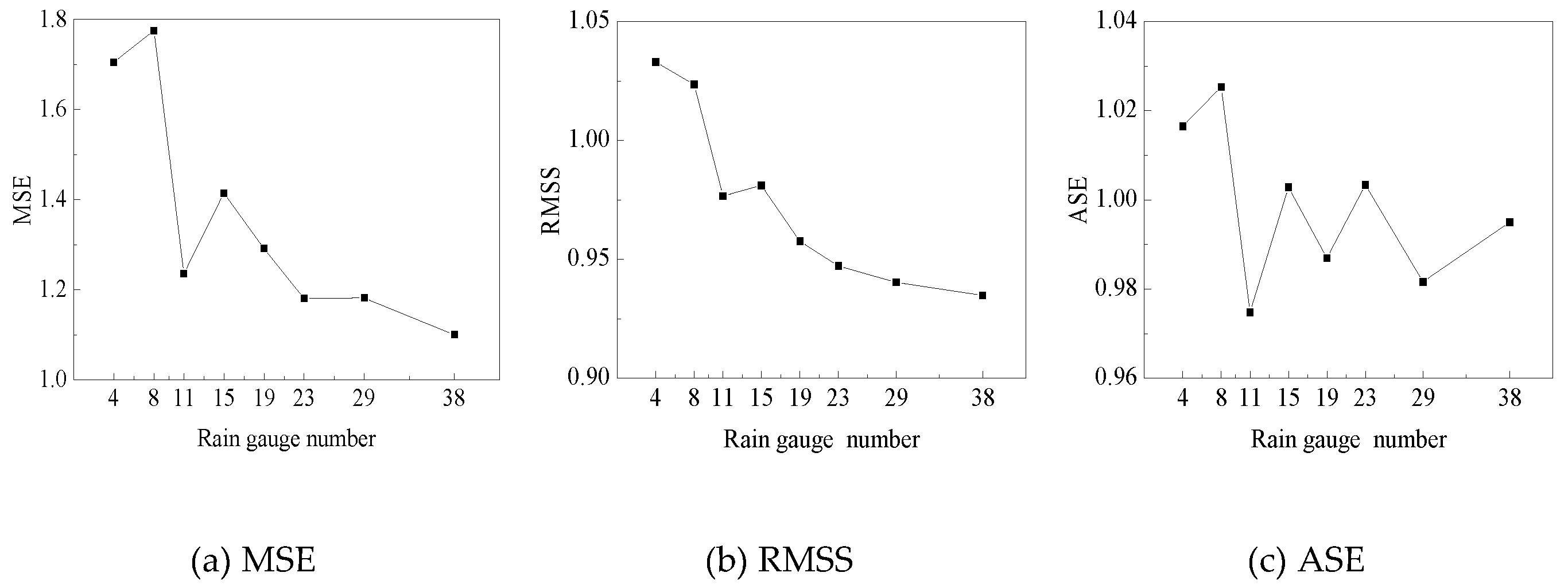
Based on the monthly rainfall value of the 38 rain gauges, we adopted three cross-validation statistics (MSE, RMSE, and ASE) to comprehensively compare the connection between different numbers and interpolation errors, which enabled us to ascertain the optimum number of base rain gauges. The relationship between the cross-validation statistics and the NRGs is presented in Figure 3, which shows that the indicator values of MSE, RMSS, and ASE [20] generally exhibited downward trends with the increase in the NRGs. This indicates that the NRGs had a greater impact on the accuracy of the rainfall interpolation, which is similar to the findings of relevant studies [32,35]. Xu et al. [1] and Wang et al. [32] suggested that the precision of hydrological simulation tends to be stable when the NRGs reaches a certain threshold.

From the perspective of the statistical indicators, a smaller MSE value in the results indicates a better prediction effect of the interpolation. It can be seen from Figure 3 that the MSE, RMSS, and ASE values vary significantly for 4 rain gauges in comparison to those for 11 rain gauges. The MSE values fluctuated slightly from 11 rain gauges to 38 rain gauges. The closer the value of the RMSS is to 1, the better the performance of the interpolation is. The RMSS values of the different rain gauge numbers fluctuated around 1, and a significant declining trend was observed when the NRGs was increased from 4 to 11. Moreover, the RMSS values remained stable when there were 11 or more rain gauges. A smaller ASE value indicates a better interpolation accuracy. The ASE value was relatively small for 11 rain gauges. This is because we randomly selected 100 combinations for each rain gauge number level, and the average statistical indicators were obtained for different rain gauge numbers. We found that the ASE value based on the interpolation results of 38 rain gauges was not very small because the rain gauges were unevenly distributed. However, the ASE value would have been larger for a network with less rain gauges. This is similar to the study by Muhamad et al. [36], who found that the value of evaluation index was not necessarily the smallest obtained at the maximum or minimum NRGs. Actually, their lower values of these statistical indices generally occurred between the minimum and maximum NRGs. Therefore, considering construction and maintenance costs, 11 was selected as the optimal number of base rain gauges through the analysis of three cross-validation statistics.

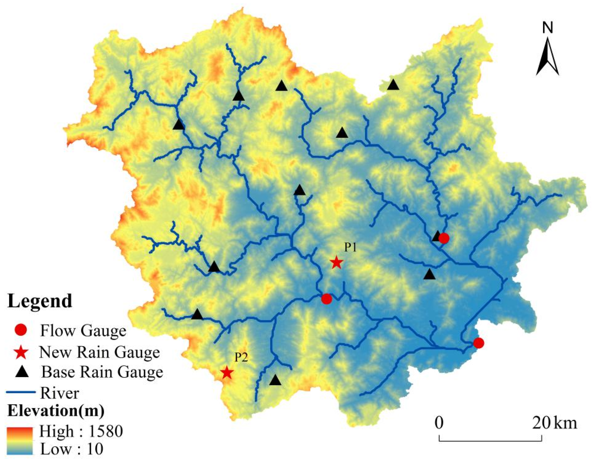
In order to further ascertain the optimal combination and location of the selected 11 rain gauges, we used the OK method to determine the distribution of the base rain gauges. The rain gauges with an MSE value close to zero were considered as those comprising the base rain gauge network. The specific distribution locations are displayed in Figure 4, which shows that 9 rain gauges were distributed in the upstream of the basin and the other two rain gauges were located in the lower reaches.

3.2. Number of New Rain Gauges Using the SCA

It can be seen from the results in Section 3.1 that, overall, the base rain gauge network could meet the required rainfall accuracy. However, there was a large estimation error of rainfall in some areas. For instance, the KSE value of some rain gauges in the basin reached a maximum of 1.20, which indicates that there was still a local monitoring gap in the base rain gauge network.

Based on above network, the NRGs, the mean distance (MD), and the mean correlation (MC) of the selected 11 gauges were calculated using the SCA. The statistics are shown in

Table 2. Statistical result of the number of rain gauges (NRGs), the mean distance (MD), and mean correlation (MC) at the rain gauges.

Distance (km)	NRGs	MD	MC
0~3	0	0	0
3~6	0	0	0
6~9	2	8.080	0.959
9~12	1	9.826	0.958
12~15	4	13.869	0.962
15~18	0	0	0
18~21	2	20.250	0.953
21~24	4	21.788	0.937
24~27	2	25.956	0.923
27~30	4	27.956	0.934
30~33	6	31.138	0.933
33~36	1	33.616	0.905
36~39	6	37.004	0.917
39~42	0	0	0
42~45	6	42.758	0.908
45~48	5	46.567	0.910
48~51	4	49.973	0.902
51~54	1	53.172	0.836
54~57	3	55.934	0.845
57~60	2	58.028	0.896
60~63	1	61.890	0.875

, which reveales that the MC decreased as the MD increased, which was consistent with the results of Bakhtiaria et al. [34]. Hence, the results could be used to plot the correlation between gauges in this study area. Moreover, we found that the MC value was largest (0.962) in the range of 12 km to 15 km, and that the MC value was not lower than 0.900 within 51 km. The correlation between the rain gauges was higher overall. In terms of the NRG value, the distance between the rain gauges with the maximum NRGs was between 30 km and 45 km. However, there was no distribution of rain gauges in the intervals of 0–6 km, 15–18 km, and 39–42 km.

As shown in Figure 5, the relationship between the MC and MD exhibited an exponential relationship. The correlation coefficient (R²) of the fitting function reached 0.7691, thus indicating that the MD and MC had a significant correlation. The correlation coefficient was similar to that reported by Nazaripour et al. [23] (R² of 0.810) and Bakhtiaria et al. [34] (R² of 0.680). Additionally, according to Equation (5), the spatial correlation function of the study area was obtained, whereby ρ₀ was 0.9838 and d₀ was 500 km.

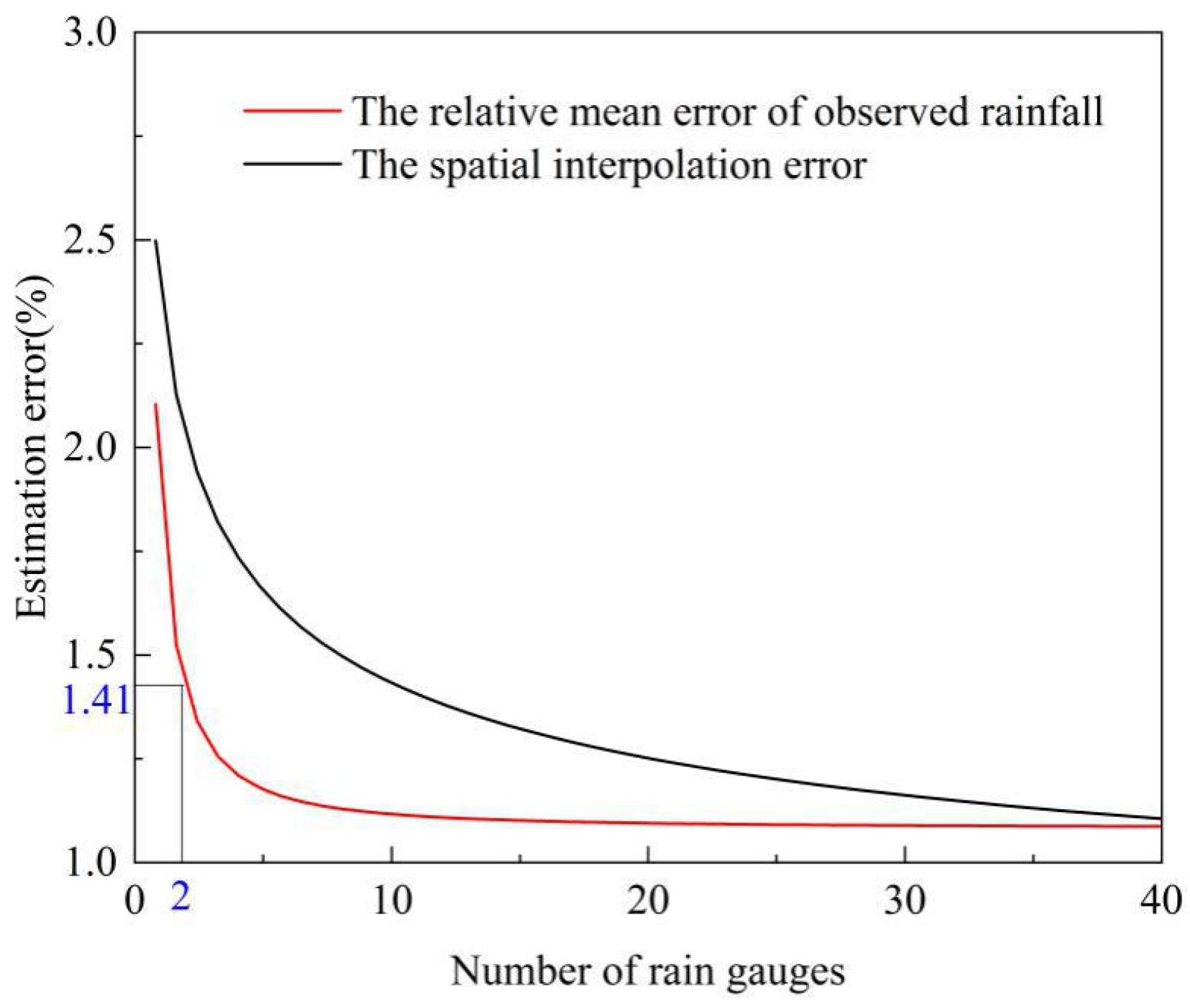
In order to obtain the amount of new rain gauges, we used E_i error criterion. When E_i was set to a confidence level of 85%, the average error of the region was 1.41% for the study area. This average error was introduced into Equation (6) and the amount of new rain gauges n was equal to two, as shown in Figure 6.

3.3. Location of New Rain Gauges Based on the OK

Fishnet, OK, and KSE maps were adopted to determine the location of the two new rain gauges (Figure 4). Xu et al. [19] indicated that it is instructive to locate unsampled rain gauges with the highest error of each grid. In the study, one new rain gauge (P1) was located near the Anxi hydrological station, and the other (P2) was located in the lower reaches of Anxi sub-basin. To verify the rationality of location of the two new rain gauges (P1 and P2), the values of three cross-validation statistics (MSE, RMSE, and ASE) for the networks of the base 11 rain gauges (N11) and the 13 rain gauges which included the base 11 rain gauges, P1 and P2 (N13_P1), were calculated based on their KSE values that obtained by the OK interpolation.

Table 3. Cross-validation statistics of the base rain gauge network and its optimal network.

Scenarios	Description	MSE	RMSE	ASE
N11	The network of base 11 rain gauges	1.5850	0.9503	0.9578
N13_P1	The network includes P1, P2 and the base 11 rain gauges	1.4559	0.9620	0.8767
N13_AX	The network includes Anxi, P2 and the base 11 rain gauges	1.5173	0.9569	0.9207

shows that the RMSS value for the N13_P1 was closer to 1 than that of the N11, whereas the MSE and ASE values were comparatively smaller. Overall, the prediction result of N13_AX was better than that of the N11. Additionally, based on the comparisons between the different rainfall gauge networks (Figure 7), it revealed that the two new rain gauges were very important for the rainfall prediction across the entire basin, and significantly reduced the interpolation error of the basin. The N13_P1 can better represent the rainfall distribution of the entire basin, which confirms the rationality of the location of the new rain gauges.

However, it is noteworthy that the new rain gauge P1 is located close to the Anxi rain gauge. The values of three cross-validation statistics (MSE, RMSE, and ASE) for the network of 13 rain gauges which included Anxi, P2, and the base 11 rain gauges (N13_AX) were also calculated. The interpolation results (Table 3) indicated that there were significant improvements in the values of MSE, RMSE, and ASE. The prediction result of the N13_P1 was better than that of N13_AX. Moreover, there are significant differences in terrain between the P1 and the Anxi gauge. To be specific, the Anxi rain gauge is located in the river valley, while the P1 is situated in the ridge with an elevation of 537 m. The study area is located in the southeast coast of China, which is often affected by water vapor from the western Pacific Ocean. The P1 is located in the windward slope and elevation is relatively high. The formation of the heavy rain gets easier as the altitude becomes higher. In contrast, the Anxi rain gauge is located at the bottom of the valley, which is unfavorable to the formation of precipitation. Furthermore, rainstorms caused by tropical weather systems, such as typhoons (i.e., typhoon rainstorm) are one of the main types of rainstorms in the Jinjiang Basin. Typhoon rainstorm centers are generally located on the half–hillside of the mountain [35,36,37,38], and the location of P1 was close to the rainstorm centers of the study area [39]. Therefore, based on the representative of stations and the requirements of disaster prevention and mitigation, we consider that the location of the new rain gauge P1 is more appropriate than that of the Anxi rain gauge.

In this study, the OK–SCA was used to optimize the current rain gauge network. It was found that the overall accuracy and local precision of the 13 rain gauges based on N13_P1 could be satisfied. For N13_P1, most of the rain gauges were distributed in the middle and upper reaches of the study area. Xu et al. [1] combined the external migration kriging method with the random sampling method to study the impact of the locations of the rain gauges on the hydrological calibration and application in the Xiangjiang River basin. The results showed that the rainfall in the high-altitude region and terrain fluctuation region was complex, and that more gauges were required to monitor the precipitation. However, less rain gauges could reflect the rainfall in plain area. Similar conclusions have been reached by Shafier et al. [12], Diodato et al. [40], and Chen et al. [41]. However, it was also found that the northeast fringe area of the Shilong sub-basin that located in the plain area and occupied almost 5% of the total area of the basin showed relatively higher errors (i.e., KSE was in range from 0.78 to 1.18). This is maybe due to the interpolation error induced by OK, the length of the period of precipitation observations, and etc. Considering the N13_P1 could provide accurate estimates of areal mean precipitation for the majority of the entire basin, it is reasonable to conclude that the feasibility and rationality of the OK–SCA for a rain gauge network optimization design. The local higher error problem could be further explored and improved in future research.

4. Conclusions

The paper designed a coupled OK–SCA for the optimization of rain gauge networks, which aims to remove redundant rain gauges and add new rain gauges to the blank monitoring areas of a basin. The application of the OK–SCA was verified through a case study of the Jinjiang Basin in the southeast coast of China. The following conclusions can be obtained from the study:

(1)

The OK method could not only identify the blank monitoring region with the highest rainfall error, but also determine the location of new rain gauges according to three cross-validation statistics (MSE, ASE, and RMSS). The SCA allowed the number of new rain gauges to be obtained. By coupling the OK and SCA, the redundant rain gauges were removed from the current rain gauge network, and new rain gauges in the blank monitoring region were determined.

(2)

The optimal rain gauge network provided more accurate rainfall estimates in comparison to the base network that was determined by the OK. The coupled OK–SCA could be appropriate for optimizing a rain gauge network in wet areas such as the Jinjiang Basin. A further study will assess how the optimized rain gauge network affects the simulation of hydrological process and the changes in hydrological model parameters.

References

1. Xu, H.; Xu, C.; Chen, H.; Zhang, Z.; Li, L. Assessing the influence of rain gauge density and distribution on hydrological model performance in a humid region of China. J. Hydrol. 2013, 505, 1–12. [Google Scholar] [CrossRef]
2. Xu, H.; Xu, C.; Sælthun, N.; Xu, Y.; Zhou, B.; Chen, H. Entropy theory based multi-criteria resampling of rain gauge networks for hydrological modelling—A case study of humid area in southern China. J. Hydrol. 2015, 525, 138–151. [Google Scholar] [CrossRef]
3. Lee, J.; Kim, S.; Jun, H. A study of the influence of the spatial distribution of rain gauge networks on areal average rainfall calculation. Water 2018, 10, 1635. [Google Scholar] [CrossRef] [Green Version]
4. Bárdossy, A.; Das, T. Influence of rainfall observation network on model calibration and application. Hydrol. Earth Syst. Sci. 2008, 12, 77–89. [Google Scholar] [CrossRef] [Green Version]
5. Xu, P.; Wang, D.; Singh, V.P.; Wang, Y.; Wu, J.; Wang, L.; Zou, X.; Chen, Y.; Chen, X.; Liu, J.; et al. A two-phase copula entropy-based multiobjective optimization approach to hydrometeorological gauge network design. J. Hydrol. 2017, 535, 228–241. [Google Scholar] [CrossRef]
6. Berne, A.; Krajewski, W. Radar for hydrology: Unfulfilled promise or unrecognized potential? Adv. Water Resour. 2013, 51, 357–366. [Google Scholar] [CrossRef]
7. Seck, I.; Baelen, J. Geostatistical Merging of a Single-Polarized X-Band Weather Radar and a Sparse Rain Gauge Network over an Urban Catchment. Atmosphere 2018, 9, 496. [Google Scholar] [CrossRef] [Green Version]
8. Chang, C.; Wu, S.; Hsu, C.; Shen, J. An evaluation framework for identifying the optimal raingauge network based on spatiotemporal variation in quantitative precipitation estimation. Hydrol. Res. 2017, 48, 77–98. [Google Scholar] [CrossRef]
9. Dai, Q.; Bray, M.; Zhuo, L.; Islam, T.; Han, D. A Scheme for Rain Gauge Network Design Based on Remotely Sensed Rainfall Measurements. J. Hydrometeorol. 2017, 18, 363–379. [Google Scholar] [CrossRef]
10. Zeng, Q.; Chen, H.; Xu, C.-Y.; Jie, M.-X.; Chen, J.; Guo, S.-L.; Liu, J. The effect of rain gauge density and distribution on runoff simulation using a lumped hydrological modelling approach. J. Hydrol. 2018, 563, 106–122. [Google Scholar] [CrossRef]
11. Peleg, N.; Ben-Asher, M.; Morin, E. Radar subpixel-scale rainfall variability and uncertainty: Lessons learned from observations of a dense rain-gauge network. Hydrol. Earth Syst. Sci. 2013, 17, 2195–2208. [Google Scholar] [CrossRef] [Green Version]
12. Shafiei, M.; Ghahraman, B.; Saghafian, B.; Pande, S.; Gharari, S.; Davary, K. Assessment of rain-gauge networks using a probabilistic GIS based approach. Hydrol. Res. 2014, 45, 551–562. [Google Scholar] [CrossRef] [Green Version]
13. Yin, Z.; Liao, W.; Lei, X.; Wang, H.; Wang, R. Comparing the Hydrological Responses of Conceptual and Process-Based Models with Varying Rain Gauge Density and Distribution. Sustainability 2018, 10, 3209. [Google Scholar] [CrossRef] [Green Version]
14. Singh, C.; Katpatal, Y. A GIS Based Design of Groundwater Level Monitoring Network Using Multi-Criteria Analysis and Geostatistical Method. Water Resour. Manag. 2017, 31, 4149–4163. [Google Scholar] [CrossRef]
15. Yuan, Y.; Yang, X.; Chen, L.; Yuan, X.; Dong, H.; Yu, Y. Optimization of the basin hydrologic network based on multi-objective criteria. J. Hohai Univ. 2019, 47, 102–107. [Google Scholar]
16. Stosic, T.; Stosic, B.; Singh, V.P. Optimizing streamflow monitoring networks using joint permutation entropy. J. Hydrol. 2017, 552, 306–312. [Google Scholar] [CrossRef]
17. Wang, W.; Wang, D.; Singh, V.P.; Wang, Y.; Wu, J.; Wang, L.; Zou, X.; Liu, J.; Zou, Y.; He, R. Optimization of rainfall networks using information entropy and temporal variability analysis. J. Hydrol. 2018, 559, 136–155. [Google Scholar] [CrossRef]
18. Huang, Y.; Zhao, H.; Jiang, Y.; Lu, X.; Duan, H.; He, R. Comparison and analysis of different discrete methods and entropy-based methods in rain gauge network design. Water 2019, 11, 1357. [Google Scholar] [CrossRef] [Green Version]
19. Xu, P.; Wang, D.; Singh, V.P.; Wang, Y.; Wu, J.; Wang, L.; Zou, X.; Liu, J.; Zou, Y.; He, R. A kriging and entropy-based approach to raingauge network design. Environ. Res. 2018, 161, 61–75. [Google Scholar] [CrossRef]
20. Adhikary, S.K.; Yilmaz, A.G.; Muttil, N. Optimal design of rain gauge network in the Middle Yarra River catchment, Australia. Hydrol. Process. 2015, 29, 2582–2599. [Google Scholar] [CrossRef] [Green Version]
21. Barca, E.; Passarella, G.; Uricchio, V. Optimal extension of the rain gauge monitoring network of the Apulian Regional Consortium for Crop Protection. Environ. Monit. Assess. 2008, 145, 375–386. [Google Scholar] [CrossRef] [PubMed]
22. Chen, Y.; Wei, C.; Yeh, H. Rainfall network design using kriging and entropy. Hydrol. Process. 2010, 22, 340–346. [Google Scholar] [CrossRef]
23. Nazaripour, H.; Mansouri, D. Rain gauge network evaluation and optimal design using spatial correlation approach in arid and semi-arid regions of Iran. Theor. Appl. Climatol. 2016, 129, 1255–1261. [Google Scholar] [CrossRef]
24. Wu, J.; Chen, X.; Yao, H.; Gao, L.; Chen, Y.; Liu, M. Non-linear relationship of hydrological drought responding to meteorological drought and impact of a large reservoir. J. Hydrol. 2017, 551, 495–507. [Google Scholar] [CrossRef]
25. Chen, Y.; Chen, X.; Xu, C.; Zhang, M.; Liu, M.; Gao, L. Toward Improved Calibration of SWAT Using Season-Based Multi-Objective Optimization: A Case Study in the Jinjiang Basin in Southeastern China. Water Resour. Manag. 2018, 32, 1193–1207. [Google Scholar] [CrossRef]
26. Zhang, J.; Li, Y. Spatial interpolation of annual precipitation data in Cambodia based on geostatistics. Yangtze River. 2018, 49, 100–103. [Google Scholar]
27. Chen, H.; Huo, R.; Zeng, Q.; Yang, W.; Chen, J.; Guo, S.; Xu, C. Comparative study on the influence of rain-gauge network on the uncertainty of hydrological modeling. Adv. Water Sci. 2019, 30, 34–44. [Google Scholar]
28. Bayat, B.; Nasseri, M.; Hosseini, K.; Karami, H. Revisited rainfall network design: Evaluation of heuristic versus entropy theory methods. Arab. J. Geosci. 2018, 11, 561. [Google Scholar] [CrossRef]
29. Haggag, M.; Elsayed, A.A.; Awadallah, A.G. Evaluation of rain gauge network in arid regions using geostatistical approach: Case study in northern Oman. Arab. J. Geosci. 2016, 9, 552. [Google Scholar] [CrossRef]
30. Amin, M.A.; Torkan, G.; Eslamian, S.; Zareian, M.J.; Adamowski, J.F. Analysis of deterministic and geostatistical interpolation techniques for mapping meteorological variables at large watershed scales. Acta Geophys. 2019, 67, 191–203. [Google Scholar] [CrossRef]
31. Foehn, A.; Hernández, J.G.; Schaefli, B.; Cesare, G.de. Spatial interpolation of precipitation from multiple rain gauge networks and weather radar data for operational applications in Alpine catchments. J. Hydrol. 2018, 563, 1092–1110. [Google Scholar] [CrossRef]
32. Wang, Q.; Yang, X.; Chen, H.; Xu, C.; Zeng, Q.; Xu, J. Influence of rain gauges network configuration on the accuracy of rainfall spatial interpolation and hydrological modeling. J. Yangtze River. Sci. Res. Inst. 2019, 36, 19–26. [Google Scholar]
33. Kagan, R.L. Planning the spatial distribution of hydrometeorological stations to meet an error criterion. In Casebook on Hydrological Network Design Practice, III-1.2; WMO Publication: Geneva, Switzerland, 1972; Volume 324. [Google Scholar]
34. Bakhtiaria, B.; Nekooamal Kermani, M.; Bordbarc, M.H. Rain Gauge Station Network Design for Hormozgan Province in Iran. Desert 2013, 18, 45–52. [Google Scholar]
35. James, E.J.; Sreedharan, K.E. Design of rain-gauge network using spatial correlation for the Bharathapuzha basin on the Malabar Coast of India. In Integrated Design of Hydrological Networks, Proceedings of the Fourth International Symposium on Inventories, Budapest, Hungary, 25–29 August 1986; IAHS Press: Madrid, Spain, 1986; Volume 158. [Google Scholar]
36. Ali, M.Z.M.; Othman, F. Rain gauge network optimization in a tropical urban area by coupling cross-validation with the geostatistical technique. Hydrol. Sci. J. 2018, 63, 474–491. [Google Scholar] [CrossRef]
37. Jiang, X.; Ren, F.; Li, J.; Qiu, Y.; Ma, Z.; Cai, B. Characteristics and Preliminary Causes of Tropical Cyclone Extreme Rainfall Events over Hainan Island. Adv. Atmos. Sci. 2018, 35, 580–591. [Google Scholar] [CrossRef]
38. Lin, Y.-F.; Wu, C.-C.; Yen, T.-H.; Huang, Y.-H.; Lien, G.-Y. Typhoon Fanapi (2010) and its Interaction with Taiwan Terrain-Evaluation of the Uncertainty in Track, Intensity and Rainfall Simulations. J. Meteorol. Soc. Jpn. 2020, 98, 93–113. [Google Scholar] [CrossRef] [Green Version]
39. Lin, Z.; Chen, X.; Lin, M.; Chen, Y. Spatial and temporal Variations of Storm-floods in Xixi Watershed of Southeast Coastal Region. Mt. Res. 2017, 35, 488–495. [Google Scholar]
40. Diodato, N. The influence of topographic co-variables on the spatial variability of precipitation over small regions of complex terrain. Int. J. Clim. 2005, 25, 351–363. [Google Scholar] [CrossRef]
41. Chen, L.; Liu, Q.; Hao, F. Impact of Network Density and Topography on Simulated Water and Sediment Yields. J. Soil Water Conserv. 2005, 19, 18–21. [Google Scholar]
Figure 1. Location of the rain gauges in the Jinjiang Basin.
Water 12 02252 g001
Figure 2. Framework for optimizing the network of rain gauges.
Water 12 02252 g002
Figure 3. Three cross-validation statistics of MSE (a), RMSS (b) and ASE (c) under different rain gauge numbers combination.
Water 12 02252 g003
Figure 4. Optimal rain gauge network based on the OK–SCA.
Water 12 02252 g004
Figure 5. Scatter plots of the MC and MD between rain gauges.
Water 12 02252 g005
Figure 6. Number of rain gauges against estimation errors for the Jinjiang Basin.
Water 12 02252 g006
Figure 7. Kriging standard error (KSE) maps for the rain gauge networks. (a) Base rain gauge network (N11); (b) Optimal rain gauge network (N13_P1); (c) Original rain gauge network.
Water 12 02252 g007