Experimental Study on the Effect of Heat-Retaining and Diversion Facilities on Thermal Discharge from a Power Plant

Abstract
:1. Introduction
2. Project Overview
3. Materials and Methods
3.1. Model Design
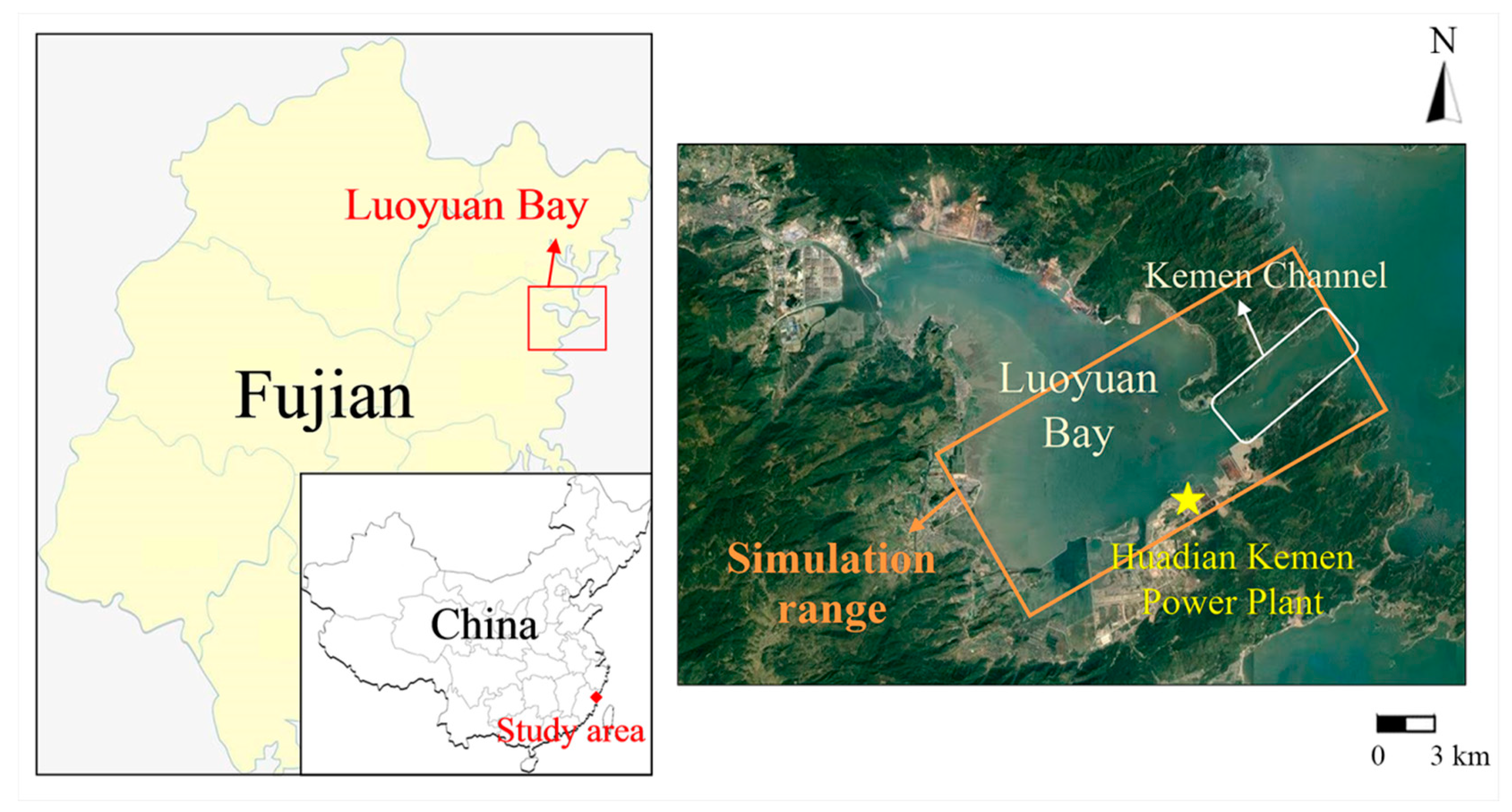
- For wide and shallow waters, it is necessary to adjust the model scale and use the distorted physical model [24,25]. Factors such as the simulation range, terrain condition, laboratory size and water supply capacity should be considered in determining the distorted scale. Due to the great amount of heated water discharged from the Huadian Kemen Power Plant and strong heat accumulation in Luoyuan Bay, the simulation range is relatively large. Generally, the average isotherm of 0.3 °C should be included in the model area. Based on the early numerical simulation results [26], the simulation range of 20 km × 8 km was determined (see Figure 1). Because of the great topographic variation and the large shoal waters in the range, the distortion ratio cannot be too small. However, considering the mixing properties in the near zone, a large distortion should also be avoided [27]. Finally, the distorted scale of 3.33 was selected with a horizontal scale of 400 and a vertical scale of 120 by comprehensive consideration.
- The model was designed according to the Froude number similarity (Equation (1)), and it was also required to meet the densimetric Froude number similarity (buoyancy effect, Equation (2)) [28,29,30].where Fr is Froude number, Fd is densimetric Froude number, V is velocity, g is gravity acceleration, H is water depth, ρ is fluid density, ∆ρ is the density difference between heated water and ambient water and the subscript “r” denotes the ratio between prototype and model.
3.2. Model Set-Up
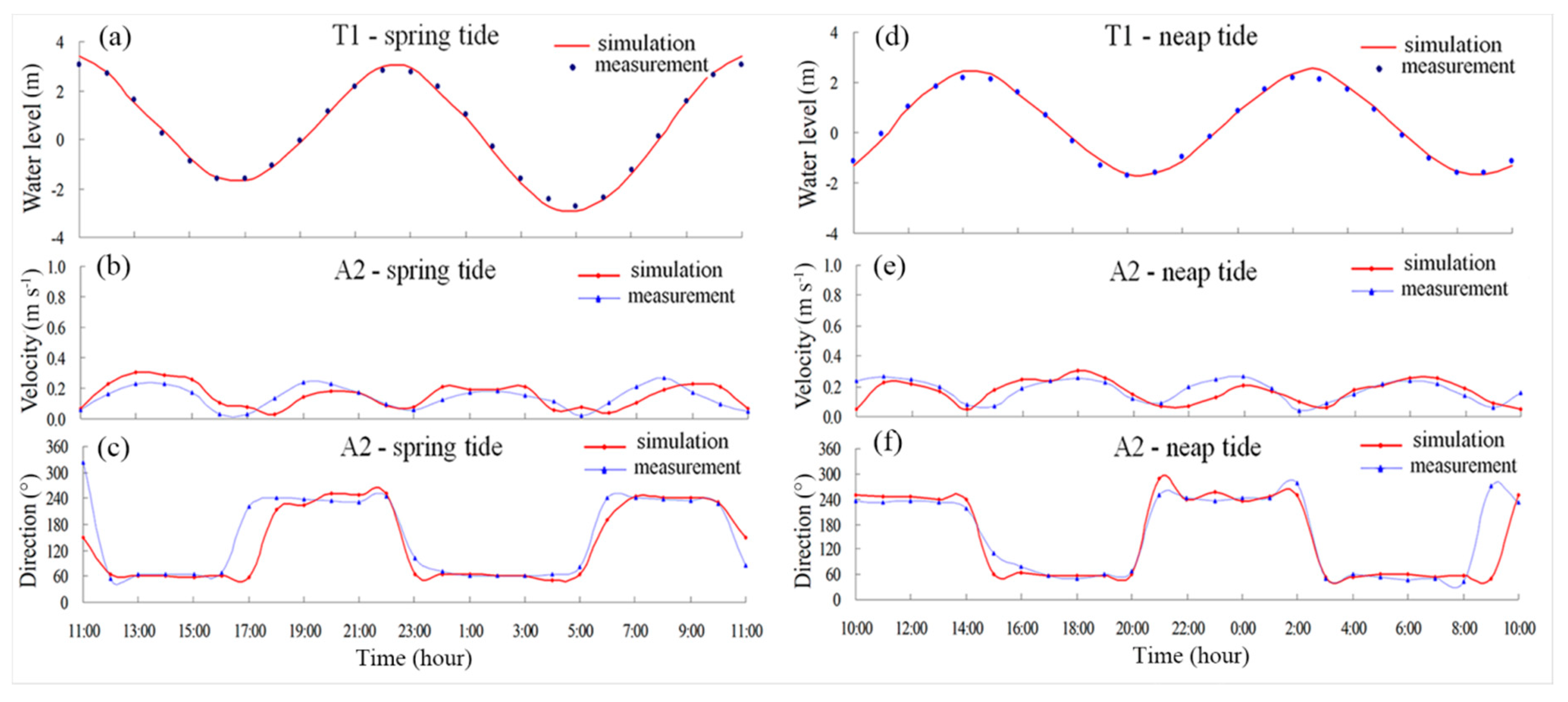
3.3. Model Validation
4. Model Scenarios
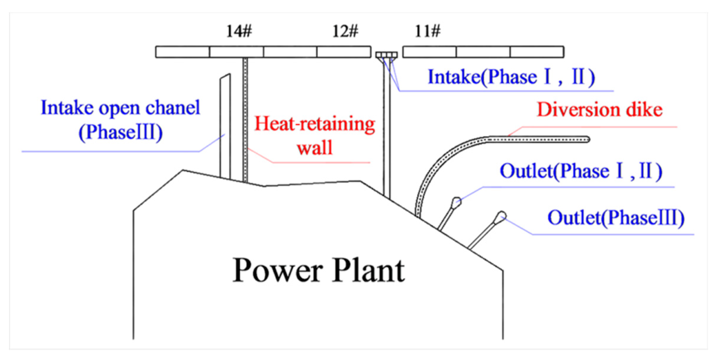
4.1. Layout Principle of Heat-Retaining and Diversion Facilities
4.2. Scenario Description
5. Results and Discussion
5.1. Thermal Properties without the Constructions
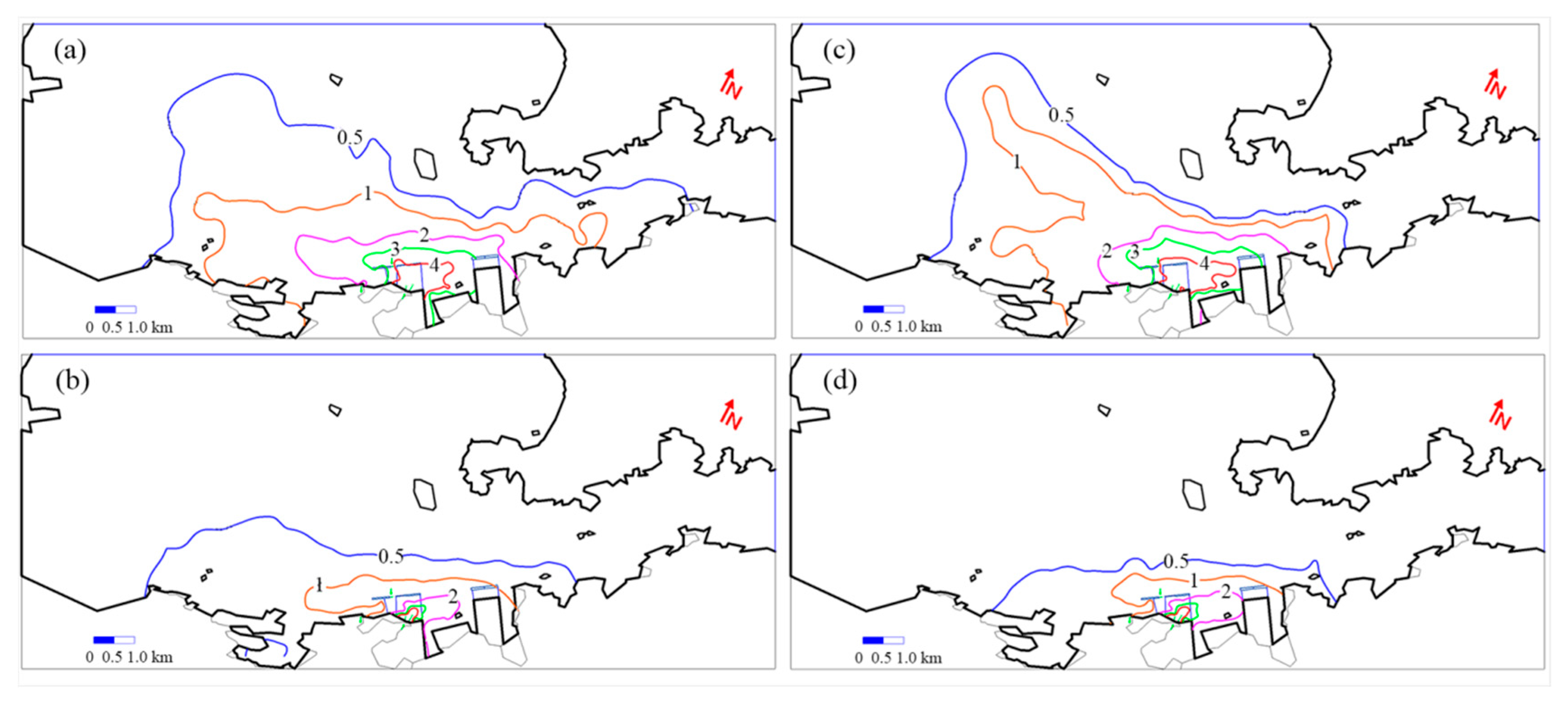
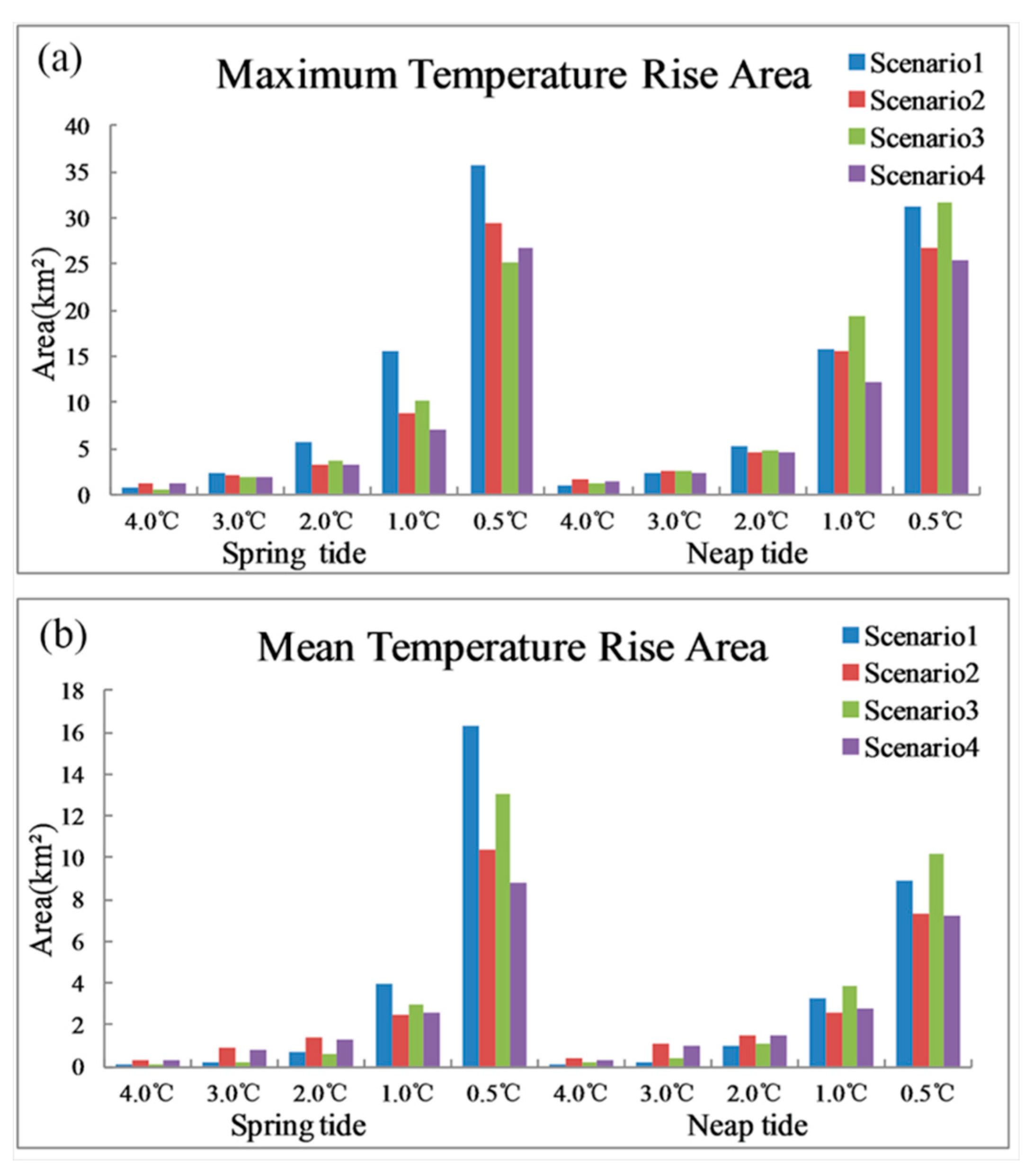
5.2. Effect of Heat-Retaining and Diversion Facilities on Temperature Rise Distribution
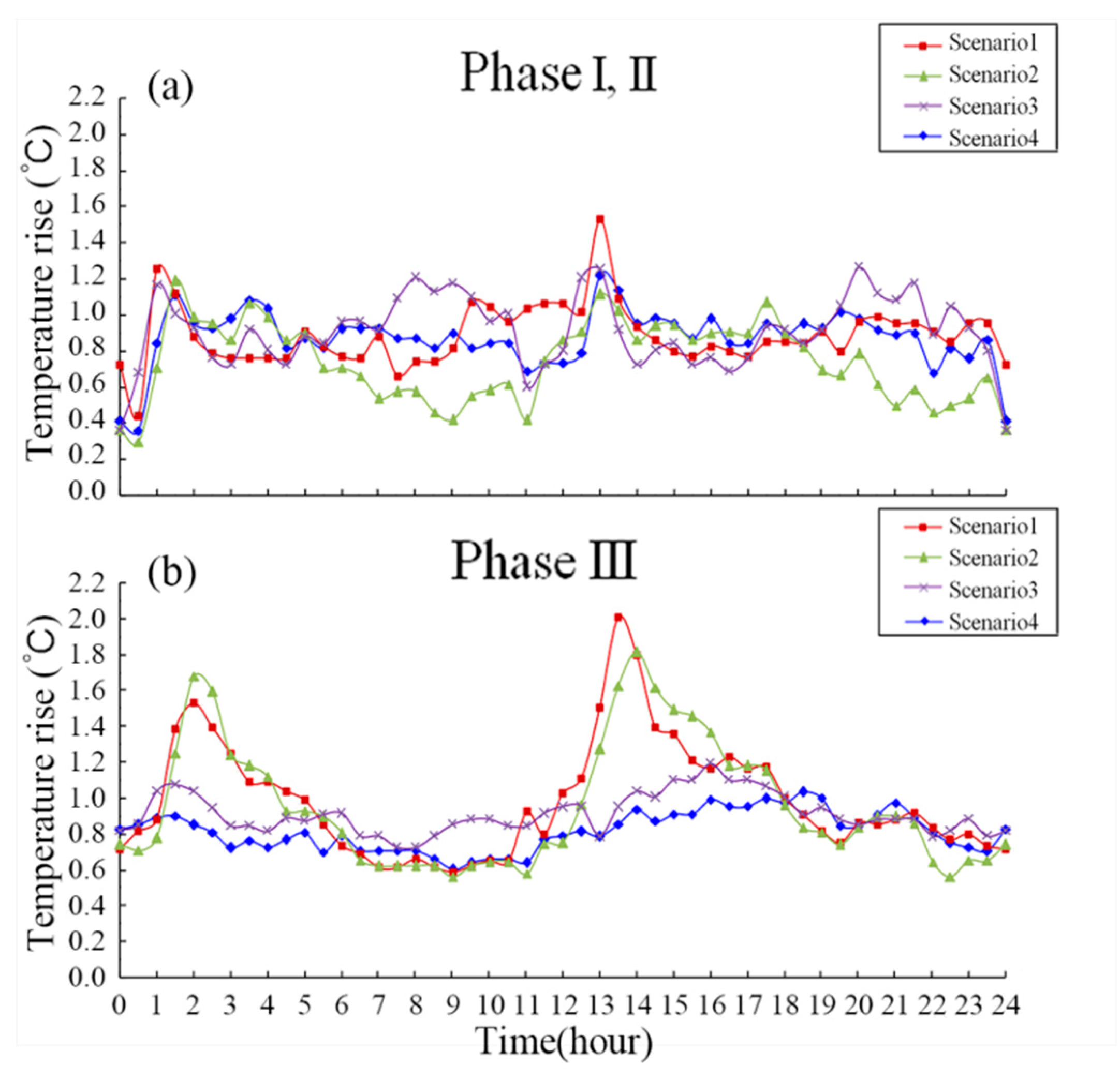
5.3. Effect of Heat-Retaining and Diversion Facilities on Excess Temperature at Intake
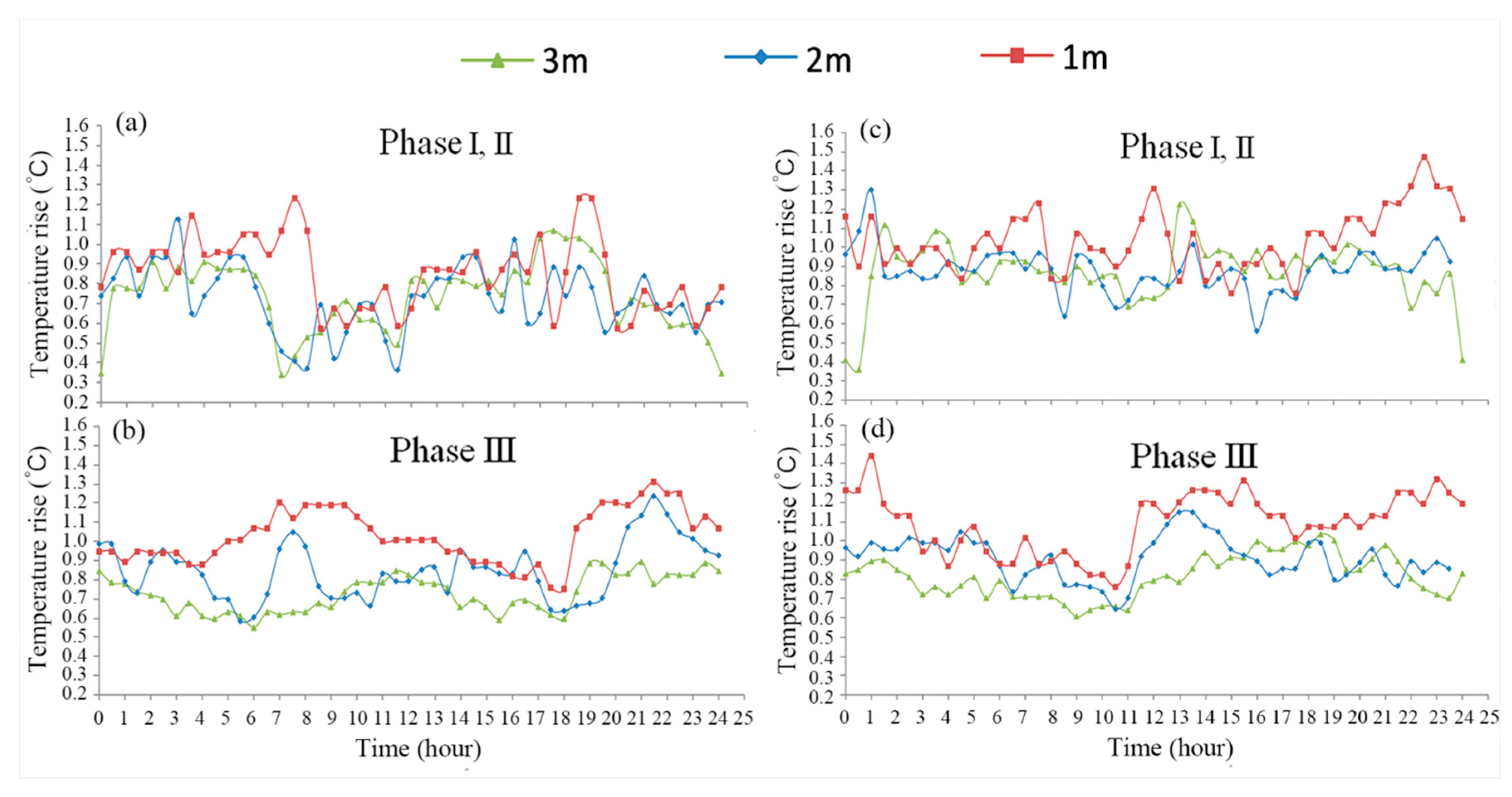
5.4. Effect of Construction Height on Excess Temperature at Intake
6. Conclusions
- Heat-retaining and diversion facilities could prevent the heated water from spreading upstream during flood tide, and effectively reduce the heat direct return. The diversion dike also promotes heat transport to outside the bay. The heat-retaining and diversion facilities strengthen the vertical mixing near the plant and weaken the thermal stratification. Therefore, they have certain impacts on the heat distribution and intake temperature rise.
- The heat-retaining and diversion facilities successfully reduced the intake temperature rise and complied with the intake requirement. Due to the different construction positions and functions, the diversion dike and the heat-retaining wall mainly reduced the intake temperature rise of prophase and Phase III, respectively. When the diversion dike and heat-retaining wall were both constructed, the greatest effects of superposition were obtained. The maximum of Phase III decreased significantly by 1.0–1.3 °C with an average reduction of 0.2 °C, and the maximum of Phase I and II decreased by 0.3 °C with little mean change.
- From an economic perspective, the crest elevations of 2 m and 1 m were considered and compared with 3 m to analyze the impact of height. The results show that when the crest elevation was reduced to 2 m, due to the short overtopping time of 4–6 h the intake temperature rise of Phase I and II had no obvious change and the average temperature rise of Phase III increased by 0.1 °C. The constructions with 2 m crest elevations still played an effective role in reducing heat return.
- The construction of heat-retaining and diversion facilities could effectively reduce the area of low temperature rise. Compared with no facilities, the maximum area of 1 °C was reduced by 3.6–8.5 km2 with a decrease of 39% and the average area of 1 °C was reduced by 0.5–1.3 km2 with a decrease of 24%. However, the area of high temperature rise became larger, and the influence of the diversion dike near the outfall was more obvious. Because the heat-retaining wall was far away from the outlet, it had little effect. The change range of the maximum area of 4 °C was less than 20%, and the average area variation of 4 °C was unapparent.
- The experimental results are valuable for the study of thermal discharge and the construction of heat-retaining and diversion facilities in similar waters. However, this paper has focused on heat transport, and other factors involved in the engineering layout should be considered overall.
Author Contributions
Funding
Acknowledgments
Conflicts of Interest
References
- Sarafraz, M.M.; Jafarian, M.; Arjomandi, M.; Nathan, G. Potential use of liquid metal oxides for chemical looping gasification: A thermodynamic assessment. Appl. Energy 2017, 195, 702–712. [Google Scholar]
- Sarafraz, M.M.; Jafarian, M.; Arjomandi, M.; Nathan, G. The relative performance of alternative oxygen carriers for liquid chemical looping combustion and gasification. Int. J. Hydrogen Energy 2017, 42, 16396–16407. [Google Scholar]
- Sarafraz, M.M.; Jafarian, M.; Arjomandi, M.; Nathan, G. Potential of molten lead oxide for liquid chemical looping gasification (LCLG): A thermochemical analysis. Int. J. Hydrogen Energy 2018, 43, 4195–4210. [Google Scholar]
- Kirillin, G.; Shatwell, T.; Kasprzak, P. Consequences of thermal pollution from a nuclear plant on lake temperature and mixing regime. J. Hydrol. 2013, 496, 47–56. [Google Scholar] [CrossRef]
- Huang, F.; Lin, J.; Zheng, B. Effects of Thermal Discharge from Coastal Nuclear Power Plants and Thermal Power Plants on the Thermocline Characteristics in Sea Areas with Different Tidal Dynamics. Water 2019, 11, 2577. [Google Scholar] [CrossRef] [Green Version]
- Love, R.V.; Alfred, W.; Damien, B. Physical effects of thermal pollution in lakes. Water Resour. Res. 2017, 53, 3968–3987. [Google Scholar]
- Lin, J.; Zou, X.; Huang, F. Effects of the thermal discharge from an offshore power plant on plankton and macrobenthic communities in subtropical China. Mar. Pollut. Bull. 2018, 131, 106–114. [Google Scholar] [CrossRef]
- Rosen, M.A.; Bulucea, C.A.; Mastorakis, N.E.; Bulucea, C.; Jeles, A.; Brindusa, C.C. Evaluating the Thermal Pollution Caused by Wastewaters Discharged from a Chain of Coal-Fired Power Plants along a River. Sustainability 2015, 7, 5920–5943. [Google Scholar] [CrossRef] [Green Version]
- Jung, Y.H.; Kim, H.J.; Park, H.S. Thermal discharge effects on the species composition and community structure of macrobenthos in rocky intertidal zone around the Taean thermoelectric power plant, Korea. Ocean Polar Res. 2018, 40, 59–67. [Google Scholar]
- Muthulakshmi, A.L.; Natesan, U.; Ferrer, V.A.; Deepthi, K.; Venugopalan, V.P.; Narasimhan, S.V. Impact assessment of nuclear power plant discharge on zooplankton abundance and distribution in coastal waters of Kalpakkam, India. Ecol. Process. 2019, 8, 22. [Google Scholar] [CrossRef] [Green Version]
- Levin, A.A.; Birch, T.J.; Hillman, R.E.; Raines, G.E. Thermal discharges. Ecological effects. Environ. Sci. Technol. 1972, 6, 224–230. [Google Scholar] [CrossRef]
- Gaeta, M.G.; Samaras, A.; Archetti, R. Numerical investigation of thermal discharge to coastal areas: A case study in South Italy. Environ. Model. Softw. 2020, 124, 104596. [Google Scholar] [CrossRef]
- Wu, J.; Buchak, E.; Edinger, J.; Kolluru, V. Simulation of cooling-water discharges from power plants. J. Environ. Manag. 2001, 61, 77–92. [Google Scholar] [CrossRef] [PubMed]
- Attia, S.I. The influence of condenser cooling water temperature on the thermal efficiency of a nuclear power plant. Ann. Nucl. Energy 2015, 80, 371–378. [Google Scholar] [CrossRef]
- Shawky, Y.; Nada, A.M.; Abdelhaleem, F.S. Environmental and hydraulic design of thermal power plants outfalls “Case study: Banha Thermal Power Plant, Egypt”. Ain Shams Eng. J. 2013, 4, 333–342. [Google Scholar] [CrossRef] [Green Version]
- Tian, C.; Cheng, Q.; Hao, R.; Zhang, C.; Tang, H. Experimental Study of Influence on Temperature Rise Due to Retraction of Water Intake in Cooling Water Engineering. Adv. Water Resour. Hydraul. Eng. 2009, VOLS 1-6, 1235–1239. [Google Scholar]
- El-Ghorab, E.A. Physical model to investigate the effect of the thermal discharge on the mixing zone (Case Study: North Giza Power Plant, Egypt). Alex. Eng. J. 2013, 52, 175–185. [Google Scholar] [CrossRef] [Green Version]
- Zeng, P.; Chen, H.; Ao, B.; Ji, P.; Wang, X.; Ou, Z. Transport of waste heat from a nuclear power plant into coastal water. Coast. Eng. 2002, 44, 301–319. [Google Scholar] [CrossRef]
- Shah, V.; Dekhatwala, A.; Banerjee, J.; Patra, A.K. Analysis of dispersion of heated effluent from power plant: A case study. Sadhana 2017, 42, 557–574. [Google Scholar] [CrossRef] [Green Version]
- Shawky, Y.M.; Ezzat, M.B.; Abdellatif, M.M. Power plant intakes performance in low flow water bodies. Water Sci. Technol. 2015, 29, 54–67. [Google Scholar] [CrossRef] [Green Version]
- Salehi, M. Thermal Recirculation Modeling for Power Plants in an Estuarine Environment. J. Mar. Sci. Eng. 2017, 5, 5. [Google Scholar] [CrossRef] [Green Version]
- Zhang, X.; Dou, X.; Chen, L.; Li, T.; Gao, X.; Li, X. Comparative analysis of the influence of different power plant intake and drainage arrangements on environments in tidal regions. J. Harbin Eng. Univ. 2019, 40, 718–723. [Google Scholar]
- Ti-Lai, L.; Li-Ming, C.; Xiang-Yu, G.; Xin-Zhou, Z.; Suh, K.-D.; Cruz, E.C.; Tajima, Y. Numerical Modeling of Thermal Discharge of Lamu Power Plant, Kenya. In Proceedings of the Asian and Pacific Coasts 2017; World Scientific: Singapore, 2017; pp. 894–903. [Google Scholar]
- Hao, R. Geometric distortion problem on the experiment of cooling water circulation model. J. Taiyuan Univ. Technol. 1999, 3, 40–43. (In Chinese) [Google Scholar]
- Valentin, H. Scale effects in physical hydraulic engineering models. J. Hydraul. Res. 2011, 49, 293–306. [Google Scholar]
- Li, H. Numerical simulation and engineering applications of thermal effluent about cooling water in tidal area. Taiyuan Univ. Technol. 2006, 6, 1–82. (In Chinese) [Google Scholar]
- Sharp, J.J. Spread of buoyant jets at the free surface. J. Hydraul. Division-ASCE 1969, 95, 811–825. [Google Scholar]
- Chen, H. Study on simulation of cooling water circulation. J. Hydraul. Eng. 1988, 11, 1–9. (In Chinese) [Google Scholar]
- Parker, F.L.; Krenkel, P.A.; Stevens, D.B. Physical and engineering aspects of thermal pollution. Crit. Rev. Environ. Sci. Technol. 1970, 1, 101–192. [Google Scholar] [CrossRef]
- Nystrom, J.B.; Hecker, G.E.; Moy, H.C. Closure to “Heated Discharge in an Estuary: Case Study” by James B. Nystrom, George E. Hecker and Han C. Moy (November, 1981). J. Hydraul. Eng. 1983, 109, 777–778. [Google Scholar] [CrossRef]
- Sun, C.; Guo, Y.; Zhao, K. Numerical simulation of tidal current in Luoyuan Bay. Mar. Sci. 2005, 29, 19–22. (In Chinese) [Google Scholar]
- Hu, J. Tidal current and residual current in Luoyuan Bay. Mar. Environ. Sci. 1996, 15, 12–16. (In Chinese) [Google Scholar]
- Fu, Z.; Hu, J. Distribution features of tidal current, residual current and temperature in Luoyuan Bay. J. Xiamen Univ. Nat. Sci. 1989, S1, 28–33. (In Chinese) [Google Scholar]
- Yu, N.; Lin, J.G.; Guo, W.-J.; Lu, J. Numerical Simulation of Heavy Metal (Pb) Distribution in Luoyuan Bay Based on Tidal Current. Adv. Mater. Res. 2012, 518, 1942–1947. [Google Scholar] [CrossRef]
- He, Y. Discussion on utilization of surplus heat of circulating cooling water of fossil fuel/nuclear power plants. J. Chin. Inst. Water Resour. Hydropower Res. 2004, 2, 315–320. (In Chinese) [Google Scholar]

 ) and velocity sites (
  ); (b) temperature probes (
  ). (
). (  : the open boundary with the pumps).
) and velocity sites ( ); (b) temperature probes ( ). ( : the open boundary with the pumps).
: the open boundary with the pumps).
) and velocity sites ( ); (b) temperature probes ( ). ( : the open boundary with the pumps).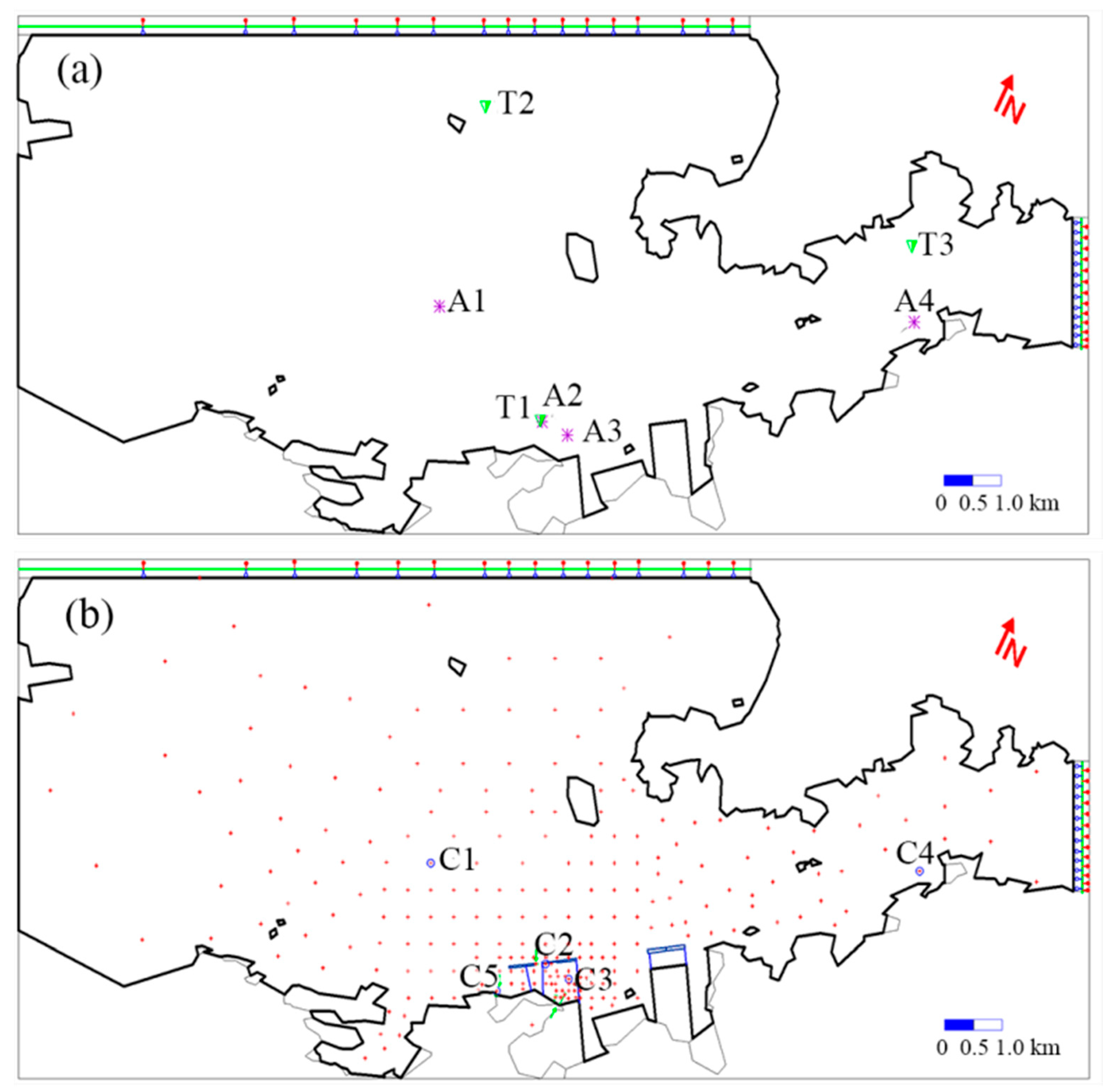


| Parameter | Notation | Value | Parameter | Notation | Value |
|---|---|---|---|---|---|
| Horizontal scale | Lr | 400 | Time scale | tr | 36.51 |
| Vertical scale | Hr | 120 | Discharge scale | Qr | 525,600 |
| Velocity scale | Vr | 10.95 | Roughness scale | nr | 1.22 |
| Temperature Rise | Surface | Depth Average (above 6 m) | ||||
|---|---|---|---|---|---|---|
| Maximum | Minimum | Mean | Maximum | Minimum | Mean | |
| Simulation (°C) | 2.10 | 0.17 | 0.73 | 1.12 | 0.17 | 0.48 |
| Measurement (°C) | 1.77 | 0.00 | 0.86 | 1.05 | 0.00 | 0.48 |
| Relative error (%) | 18.6 | / | 15.1 | 6.7 | / | 0 |
| Scenario | Tidal Type | Height (m) | Layout Instruction | Others |
|---|---|---|---|---|
| 1 | Spring tide | 3 | Without heat-retaining and diversion facilities | Phase I, II and III; cooling water of 147.34 m3 s−1; temperature rise at outlet of 8.5 °C |
| Neap tide | ||||
| 2 | Spring tide | 3 | With diversion dike | |
| Neap tide | ||||
| 3 | Spring tide | 3 | With heat-retaining wall | |
| Neap tide | ||||
| 4 | Spring tide | 3 | With diversion dike and heat-retaining wall | |
| Neap tide | ||||
| 4-1 | Spring tide | 2 | With diversion dike and heat-retaining wall | |
| Neap tide | ||||
| 4-2 | Spring tide | 1 | With diversion dike and heat-retaining wall | |
| Neap tide |
| Scenario | Tide Type | Phase I, II (°C) | Phase III (°C) | ||||
|---|---|---|---|---|---|---|---|
| Maximum | Minimum | Mean | Maximum | Minimum | Mean | ||
| 1 | Spring tide | 1.34 | 0.41 | 0.75 | 2.15 | 0.61 | 0.97 |
| Neap tide | 1.53 | 0.44 | 0.90 | 2.10 | 0.59 | 0.98 | |
| 2 | Spring tide | 1.01 | 0.35 | 0.66 | 1.79 | 0.45 | 0.85 |
| Neap tide | 1.19 | 0.30 | 0.75 | 1.80 | 0.56 | 0.95 | |
| 3 | Spring tide | 1.31 | 0.27 | 0.84 | 1.10 | 0.63 | 0.82 |
| Neap tide | 1.27 | 0.36 | 0.92 | 1.19 | 0.73 | 0.91 | |
| 4 | Spring tide | 1.07 | 0.33 | 0.74 | 0.89 | 0.55 | 0.72 |
| Neap tide | 1.22 | 0.36 | 0.89 | 1.03 | 0.60 | 0.81 | |
© 2020 by the authors. Licensee MDPI, Basel, Switzerland. This article is an open access article distributed under the terms and conditions of the Creative Commons Attribution (CC BY) license (http://creativecommons.org/licenses/by/4.0/).
Share and Cite
Hao, R.; Qiao, L.; Han, L.; Tian, C. Experimental Study on the Effect of Heat-Retaining and Diversion Facilities on Thermal Discharge from a Power Plant. Water 2020, 12, 2267. https://doi.org/10.3390/w12082267
Hao R, Qiao L, Han L, Tian C. Experimental Study on the Effect of Heat-Retaining and Diversion Facilities on Thermal Discharge from a Power Plant. Water. 2020; 12(8):2267. https://doi.org/10.3390/w12082267
Chicago/Turabian StyleHao, Ruixia, Liyuan Qiao, Lijuan Han, and Chun Tian. 2020. "Experimental Study on the Effect of Heat-Retaining and Diversion Facilities on Thermal Discharge from a Power Plant" Water 12, no. 8: 2267. https://doi.org/10.3390/w12082267