Trend Analysis of Rainfall Time Series in Shanxi Province, Northern China (1957–2019)


Abstract
:1. Introduction
2. Materials and Methods
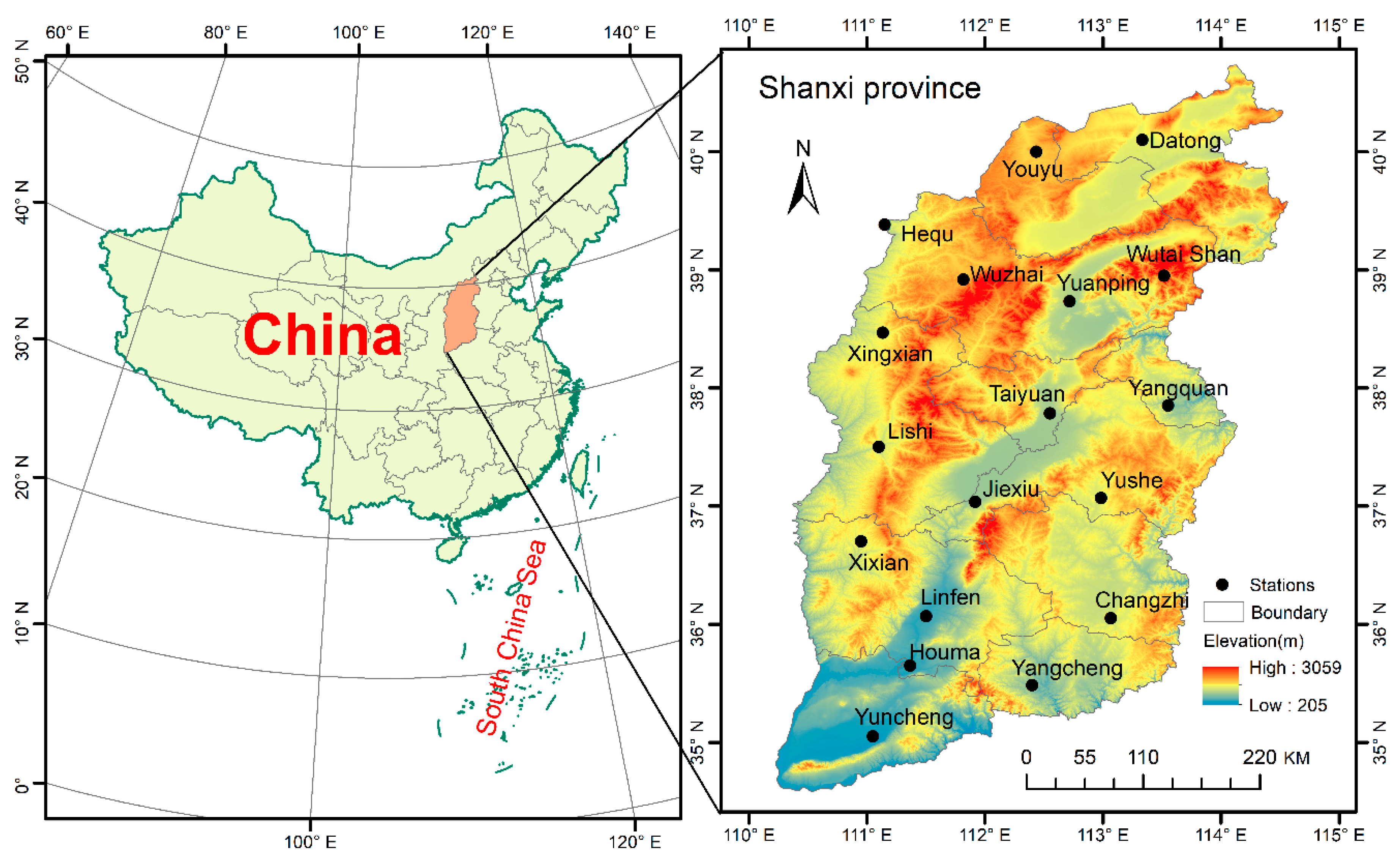
2.1. Study Area and Data Availability
2.2. Methodology
2.2.1. The Mann–Kendall Test
2.2.2. The Spearman’s Rho Test
2.2.3. Sen’s Slope Estimator
2.2.4. Serial Correlation Effect
2.2.5. The Revised Mann–Kendall Test
3. Results and Discussion
3.1. Statistical Characteristics of the Rainfall Time Series
3.2. Autocorrelation Analysis
3.3. Monthly, Seasonal, and Annual Rainfall Trend
3.4. Magnitude of Trend
3.5. Impacts of ENSO on Rainfall in Shanxi Province
4. Conclusions
- The months June and September showed no significant trends for all stations according to the MK/SR, while only September showed no significant trend using the RMK test. March experienced significant decreasing trends for most stations (Wutai shan, Yangquan, Yushe, Xixian, Jiexiu, Linfen, Changzhi, Yuncheng, Houma, and Yangcheng) at the significance levels of 10%, 5%, and 1% identified by the MK/SR and RMK tests. Only Wutai Shan station showed a significant downward trend in January, March, April, November, and December at the levels of 1% and 5% by the application of the MK/SR and RMK tests. For remaining stations, significant increasing or decreasing trends were observed in February (Wuzhai and Changzhi), April (Changzhi), May (Wuzhai), June (Datong), July (Xixian and Yuncheng), August (Yangquan and Yushe), and December (Houma).
- On the seasonal scale, similar results were obtained by using the MK/SR and RMK tests. However, the number of significant trends was increased by the application of RMK test. The values of the Z-statistic in summer at Youyu, Yuncheng, and Yangcheng stations using the RMK test showed a significant decreasing trend at the level of 10%, while those using the MK/SR test showed no significant trends. In addition, spring, summer and winter at Yuanping, Yuncheng, and Yangcheng, experienced similar changes when using the RMK test instead of the MK/SR test. Over the four seasons, both the MK/SR and RMK tests indicated that Wutai Shan station showed a significant decreasing trend at a significance level of 1% (spring, summer, and winter) and 10% (autumn). On the annual scale, most stations showed non-significant trends, except Wutai Shan, Yushe, Yuncheng, and Yangcheng, with the application of the RMK test.
- Summer showed a negative slope magnitudes for all stations. The Wutai Shan station showed the highest negative slope magnitude in the annual series (−4.224 mm/year), followed by the summer (−2.263 mm/year). Spring ranked third, with a decreasing rate of −1.067 mm/year. The magnitudes of the trend slope in January, February, and December for all stations were no trend or slightly increasing (decreasing; close to zero). A falling slope of the rainfall trend existed in July, August, October, and November.
- Both MK and SR have similar power for detecting monotonic trend in rainfall time series data. Overall, the RMK test proposed by Hamed and Rao [38] can improve the trend analysis of rainfall series by considering the autocorrelation effect at significant lags.
Author Contributions
Funding
Acknowledgments
Conflicts of Interest
References
- Huang, J.; Sun, S.; Xue, Y.; Zhang, J. Spatial and temporal variability of precipitation indices during 1961–2010 in Hunan province, central south China. Theor. Appl. Climatol. 2014, 118, 581–595. [Google Scholar] [CrossRef]
- Huang, J.; Sun, S.; Zhang, J. Detection of trends in precipitation during 1960–2008 in Jiangxi province, southeast China. Theor. Appl. Climatol. 2013, 114, 237–251. [Google Scholar] [CrossRef]
- Sanikhani, H.; Kisi, O.; Mirabbasi, R.; Meshram, S.G. Trend analysis of rainfall pattern over the central India during 1901–2010. Arabian J. Geosci. 2018, 11, 437. [Google Scholar] [CrossRef]
- Gajbhiye, S.; Meshram, C.; Mirabbasi, R.; Sharma, S.K. Trend analysis of rainfall time series for Sindh river basin in India. Theor. Appl. Clim. 2015, 125, 593–608. [Google Scholar] [CrossRef]
- Warwade, P.; Tiwari, S.; Ranjan, S.; Chandniha, S.K.; Adamowski, J. Spatio-temporal variation of rainfall over Bihar State, India. J. Water Land Dev. 2018, 36, 183–197. [Google Scholar] [CrossRef] [Green Version]
- Huang, J.; Zhang, J.; Zhang, Z.; Xu, C.-Y. Spatial and temporal variations in rainfall erosivity during 1960–2005 in the Yangtze river basin. Stoch. Environ. Res. Risk Assess. 2012, 27, 337–351. [Google Scholar] [CrossRef]
- De Luis, M.; González-Hidalgo, J.C.; Brunetti, M.; Longares, L.A. Precipitation concentration changes in Spain 1946–2005. Nat. Hazards Earth Syst. Sci. 2011, 11, 1259–1265. [Google Scholar] [CrossRef] [Green Version]
- Malik, A.; Kumar, A. Spatio-temporal trend analysis of rainfall using parametric and non-parametric tests: Case study in Uttarakhand, India. Theor. Appl. Clim. 2020, 140, 183–207. [Google Scholar] [CrossRef]
- Almazroui, M.; Islam, M.N.; Athar, H.; Jones, P.D.; Rahman, M.A. Recent climate change in the Arabian Peninsula: Annual rainfall and temperature analysis of Saudi Arabia for 1978–2009. Int. J. Clim. 2012, 32, 953–966. [Google Scholar] [CrossRef]
- Raj, P.P.N.; Azeez, P.A. Trend analysis of rainfall in Bharathapuzha River basin, Kerala, India. Int. J. Clim. 2011, 32, 533–539. [Google Scholar] [CrossRef]
- Gajbhiye, S.; Meshram, C.; Singh, S.K.; Srivastava, P.K.; Islam, T. Precipitation trend analysis of Sindh River basin, India, from 102-year record (1901–2002). Atmos. Sci. Lett. 2015, 17, 71–77. [Google Scholar] [CrossRef]
- Sivajothi, R.; Karthikeyan, K. Long-Term Trend Analysis of Changing Precipitation in Tamil Nadu, India. Int. J. Eng. Technol. 2018, 7, 980–984. [Google Scholar] [CrossRef]
- Chandniha, S.K.; Meshram, S.G.; Adamowski, J.F.; Meshram, C. Trend analysis of precipitation in Jharkhand State, India. Theor. Appl. Clim. 2016, 130, 261–274. [Google Scholar] [CrossRef]
- Altava-Ortiz, V.; Llasat, M.-C.; Ferrari, E.; Atencia, A.; Sirangelo, B. Monthly rainfall changes in Central and Western Mediterranean basins, at the end of the 20th and beginning of the 21st centuries. Int. J. Clim. 2010, 31, 1943–1958. [Google Scholar] [CrossRef]
- Bartolini, G.; Grifoni, D.; Magno, R.; Torrigiani, T.; Gozzini, B. Changes in temporal distribution of precipitation in a Mediterranean area (Tuscany, Italy) 1955–2013. Int. J. Clim. 2017, 38, 1366–1374. [Google Scholar] [CrossRef]
- Bartolini, G.; Grifoni, D.; Torrigiani, T.; Vallorani, R.; Meneguzzo, F.; Gozzini, B. Precipitation changes from two long-term hourly datasets in Tuscany, Italy. Int. J. Clim. 2014, 34, 3977–3985. [Google Scholar] [CrossRef]
- Brunetti, M.; Caloiero, T.; Coscarelli, R.; Gullà, G.; Nanni, T.; Simolo, C. Precipitation variability and change in the Calabria region (Italy) from a high resolution daily dataset. Int. J. Clim. 2010, 32, 57–73. [Google Scholar] [CrossRef]
- Caloiero, T.; Coscarelli, R.; Ferrari, E.; Mancini, M. Trend detection of annual and seasonal rainfall in Calabria (Southern Italy). Int. J. Clim. 2010, 31, 44–56. [Google Scholar] [CrossRef]
- Birara, H.; Pandey, R.P.; Mishra, S.K. Trend and variability analysis of rainfall and temperature in the Tana basin region, Ethiopia. J. Water Clim. Chang. 2018, 9, 555–569. [Google Scholar] [CrossRef] [Green Version]
- Chang, X.; Xu, Z.; Zhao, G.; Cheng, T.; Song, S. Spatial and temporal variations of precipitation during 1979–2015 in Jinan city, China. J. Water Clim. Chang. 2018, 9, 540–554. [Google Scholar] [CrossRef]
- Duan, A.; Wang, M.; Lei, Y.; Cui, Y. Trends in summer rainfall over china associated with the Tibetan Plateau sensible heat source during 1980–2008. J. Clim. 2013, 26, 261–275. [Google Scholar] [CrossRef] [Green Version]
- Shi, P.; Qiao, X.; Chen, X.; Zhou, M.; Qu, S.; Ma, X.; Zhang, Z. Spatial distribution and temporal trends in daily and monthly precipitation concentration indices in the upper reaches of the Huai River, China. Stoch. Environ. Res. Risk Assess. 2013, 28, 201–212. [Google Scholar] [CrossRef]
- Shi, P.; Wu, M.; Qu, S.; Jiang, P.; Qiao, X.; Chen, X.; Zhou, M.; Zhang, Z. Spatial Distribution and Temporal Trends in Precipitation Concentration Indices for the Southwest China. Water Resour. Manag. 2015, 29, 3941–3955. [Google Scholar] [CrossRef]
- Wang, Y.; Xu, Y.; Tabari, H.; Wang, J.; Wang, Q.; Song, S.; Hu, Z. Innovative trend analysis of annual and seasonal rainfall in the Yangtze River Delta, eastern China. Atmos. Res. 2020, 231, 104673. [Google Scholar] [CrossRef]
- Wu, H.; Qian, H. Innovative trend analysis of annual and seasonal rainfall and extreme values in Shaanxi, China, since the 1950s. Int. J. Clim. 2016, 37, 2582–2592. [Google Scholar] [CrossRef]
- Daniels, E.E.; Lenderink, G.; Hutjes, R.W.A.; Holtslag, A.A.M. Spatial precipitation patterns and trends in The Netherlands during 1951–2009. Int. J. Clim. 2013, 34, 1773–1784. [Google Scholar] [CrossRef]
- Park, J.-S.; Kang, H.-S.; Lee, Y.S.; Kim, M.-K. Changes in the extreme daily rainfall in South Korea. Int. J. Clim. 2010, 31, 2290–2299. [Google Scholar] [CrossRef]
- Fernandes, L.G.; Rodrigues, R.R. Changes in the patterns of extreme rainfall events in southern Brazil. Int. J. Clim. 2017, 38, 1337–1352. [Google Scholar] [CrossRef]
- Duan, Z.; Chen, Q.; Chen, C.; Liu, J.; Gao, H.; Song, X.; Wei, M. Spatiotemporal analysis of nonlinear trends in precipitation over Germany during 1951–2013 from multiple observation-based gridded products. Int. J. Climatol. 2018, 39, 2120–2135. [Google Scholar] [CrossRef]
- Druyan, L.M. Studies of 21st-century precipitation trends over West Africa. Int. J. Clim. 2010, 31, 1415–1424. [Google Scholar] [CrossRef]
- Zhang, C.; Wang, Z.; Zhou, B.; Li, Y.; Tang, H.; Xiang, B. Trends in autumn rain of West China from 1961 to 2014. Theor. Appl. Clim. 2018, 135, 533–544. [Google Scholar] [CrossRef]
- Zhang, Q.; Singh, V.P.; Li, J.; Jiang, F.; Bai, Y. Spatio-temporal variations of precipitation extremes in Xinjiang, China. J. Hydrol. 2012, 434, 7–18. [Google Scholar] [CrossRef]
- Qiang, Z.; Singh, V.P.; Peng, J.; Chen, Y.D.; Li, J. Spatial–temporal changes of precipitation structure across the Pearl River basin, China. J. Hydrol. 2012, 440, 113–122. [Google Scholar] [CrossRef]
- Yang, H.-L.; Xiao, H.; Guo, C.; Sun, Y. Spatial-temporal analysis of precipitation variability in Qinghai Province, China. Atmos. Res. 2019, 228, 242–260. [Google Scholar] [CrossRef]
- Zhang, Q.; Xu, C.; Zhang, Z.; Chen, X.; Han, Z. Precipitation extremes in a karst region: A case study in the Guizhou province, southwest China. Theor. Appl. Clim. 2009, 101, 53–65. [Google Scholar] [CrossRef]
- Zhang, Q.; Xu, C.-Y.; Zhang, Z.; Chen, Y.D.; Liu, C.-L. Spatial and temporal variability of precipitation over China, 1951–2005. Theor. Appl. Clim. 2008, 95, 53–68. [Google Scholar] [CrossRef]
- Liu, Q.; Yang, Z.; Cui, B. Spatial and temporal variability of annual precipitation during 1961–2006 in Yellow River basin, China. J. Hydrol. 2008, 361, 330–338. [Google Scholar] [CrossRef]
- Li, X.; Wang, X.; Babovic, V. Analysis of variability and trends of precipitation extremes in Singapore during 1980–2013. Int. J. Clim. 2017, 38, 125–141. [Google Scholar] [CrossRef]
- Chow, W.T. The impact of weather extremes on urban resilience to hydro-climate hazards: A Singapore case study. Int. J. Water Resour. Dev. 2017, 34, 510–524. [Google Scholar] [CrossRef] [Green Version]
- Guo, X.; Wu, Z.-F.; He, H.S.; Du, H.; Wang, L.; Yang, Y.; Zhao, W. Variations in the start, end, and length of extreme precipitation period across China. Int. J. Clim. 2017, 38, 2423–2434. [Google Scholar] [CrossRef]
- Lü, M.; Wu, S.-J.; Chen, J.; Chen, C.; Wen, Z.; Huang, Y. Changes in extreme precipitation in the Yangtze River basin and its association with global mean temperature and ENSO. Int. J. Clim. 2017, 38, 1989–2005. [Google Scholar] [CrossRef]
- Ii, M.Q.V.; Matsumoto, J.; Kubota, H.; Villafuerte, M.Q. Changes in extreme rainfall in the Philippines (1911-2010) linked to global mean temperature and ENSO. Int. J. Clim. 2014, 35, 2033–2044. [Google Scholar] [CrossRef]
- Tedeschi, R.G.; Grimm, A.M.; Cavalcanti, I.F.A. Influence of Central and East ENSO on extreme events of precipitation in South America during austral spring and summer. Int. J. Clim. 2014, 35, 2045–2064. [Google Scholar] [CrossRef]
- Dai, A.; Wigley, T.M.L. Global patterns of ENSO-induced precipitation. Geophys. Res. Lett. 2000, 27, 1283–1286. [Google Scholar] [CrossRef] [Green Version]
- Philippon, N.; Rouault, M.; Richard, Y.; Favre, A. The influence of ENSO on winter rainfall in South Africa. Int. J. Clim. 2011, 32, 2333–2347. [Google Scholar] [CrossRef]
- Räsänen, T.A.; Kummu, M. Spatiotemporal influences of ENSO on precipitation and flood pulse in the Mekong River Basin. J. Hydrol. 2013, 476, 154–168. [Google Scholar] [CrossRef]
- Hamed, K.H.; Rao, A.R. A modified Mann-Kendall trend test for autocorrelated data. J. Hydrol. 1998, 204, 182–196. [Google Scholar] [CrossRef]
- Zhao, G.X.; Zhao, C.P.; Li, X.S. Analysis of climate change in Shanxi Province in recent 47 years. Arid Zone Res. 2006, 23, 500–503. (In Chinese) [Google Scholar]
- Yang, Q.; Liu, D.F.; Meng, X.M. Spatial and temporal variation characteristics of precipitation and temperature in Shanxi Province from 1960 to 2017. Pearl River 2019, 40, 27–33. (In Chinese) [Google Scholar]
- Mann, H.B. Nonparametric Tests against Trend. Econometrica 1945, 13, 245. [Google Scholar] [CrossRef]
- Kendall, M.G. Rank Correlation Methods; Charles Griffin: London, UK, 1955. [Google Scholar]
- Patakamuri, S.K.; Muthiah, K.; Sridhar, V. Long-Term Homogeneity, Trend, and Change-Point Analysis of Rainfall in the Arid District of Ananthapuramu, Andhra Pradesh State, India. Water 2020, 12, 211. [Google Scholar] [CrossRef] [Green Version]
- Gocic, M.; Trajkovic, S. Analysis of changes in meteorological variables using Mann-Kendall and Sen’s slope estimator statistical tests in Serbia. Global Planet. Chang. 2013, 100, 172–182. [Google Scholar] [CrossRef]
- Spearman, C. The Proof and Measurement of Association between Two Things. Am. J. Psychol. 1904, 15, 72. [Google Scholar] [CrossRef]
- Yue, S.; Pilon, P.; Cavadias, G. Power of the Mann–Kendall and Spearman’s rho tests for detecting monotonic trends in hydrological series. J. Hydrol. 2002, 259, 254–271. [Google Scholar] [CrossRef]
- Theil, H. A Rank-Invariant Method of Linear and Polynomial Regression Analysis. Adv. Stud. Theor. Appl. Econom. 1992, 23, 345–381. [Google Scholar] [CrossRef]
- Sen, P.K. Estimates of the Regression Coefficient Based on Kendall’s Tau. J. Am. Stat. Assoc. 1968, 63, 1379–1389. [Google Scholar] [CrossRef]
- Anderson, R.L. Distribution of the Serial Correlation Coefficient. Ann. Math. Stat. 1942, 13, 1–13. [Google Scholar] [CrossRef]
- Sharma, S.; Singh, P.K. Long Term Spatiotemporal Variability in Rainfall Trends over the State of Jharkhand, India. Climate 2017, 5, 18. [Google Scholar] [CrossRef] [Green Version]
- Yue, S.; Pilon, P.; Phinney, B.; Cavadias, G. The influence of autocorrelation on the ability to detect trend in hydrological series. Hydrol. Process. 2002, 16, 1807–1829. [Google Scholar] [CrossRef]
- Ye, J.-S. Trend and variability of China’s summer precipitation during 1955-2008. Int. J. Climatol. 2014, 34, 559–566. [Google Scholar] [CrossRef]
- Li, X.; Zhang, K.; Babovic, V. Projections of Future Climate Change in Singapore Based on a Multi-Site Multivariate Downscaling Approach. Water 2019, 11, 2300. [Google Scholar] [CrossRef] [Green Version]
- Manocha, N.; Babovic, V. Development and valuation of adaptation pathways for storm water management infrastructure. Environ. Sci. Policy 2017, 77, 86–97. [Google Scholar] [CrossRef]
- Qiang, Z.; Li, J.; Singh, V.P.; Xu, C.; Deng, J. Influence of ENSO on precipitation in the East River basin, south China. J. Geophys. Res. Atmos. 2013, 118, 2207–2219. [Google Scholar] [CrossRef]
- Xiao, M.; Qiang, Z.; Singh, V.P. Spatiotemporal variations of extreme precipitation regimes during 1961-2010 and possible teleconnections with climate indices across China. Int. J. Clim. 2016, 37, 468–479. [Google Scholar] [CrossRef]
- Mariotti, A. How ENSO impacts precipitation in southwest central Asia. Geophys. Res. Lett. 2007, 34, 34. [Google Scholar] [CrossRef]
- Xu, Z.X.; Takeuchi, K.; Ishidaira, H. Correlation between El Niño–Southern Oscillation(ENSO) and precipitation in South-east Asia and the Pacific region. Hydrol. Process. 2004, 18, 107–123. [Google Scholar] [CrossRef]
- Yeo, S.-R.; Yeh, S.; Kim, Y.; Yim, S.-Y. Monthly climate variation over Korea in relation to the two types of ENSO evolution. Int. J. Clim. 2017, 38, 811–824. [Google Scholar] [CrossRef]
- Yeh, S.; Kim, H.; Kwon, M.; Dewitte, B. Changes in the spatial structure of strong and moderate El Niño events under global warming. Int. J. Clim. 2013, 34, 2834–2840. [Google Scholar] [CrossRef]
- Wang, H.; Asefa, T. Impact of different types of ENSO conditions on seasonal precipitation and streamflow in the Southeastern United States. Int. J. Clim. 2017, 38, 1438–1451. [Google Scholar] [CrossRef]
- Li, F.; Zhang, J.X.; Hao, Z.W.; Wu, Y.L.; Zhou, J.H. Correlation analysis of rainfall and ENSO in Shanxi. Acta Geogr. Sin. 2015, 70, 420–430. [Google Scholar]


| Station ID | Station | Latitude | Longitude | Elevation (m) | Record Period |
|---|---|---|---|---|---|
| 53478 | Youyu | 40°00′ | 112°27′ | 1345.8 | 1957–2019 |
| 53487 | Datong | 40°06′ | 113°20′ | 1067.2 | 1957–2019 |
| 53564 | Hequ | 39°23′ | 111°09′ | 861.5 | 1957–2019 |
| 53588 | Wutai Shan | 38°57′ | 113°31′ | 2208.3 | 1957–2019 |
| 53663 | Wuzhai | 38°55′ | 111°49′ | 1401 | 1957–2019 |
| 53664 | Xingxian | 38°28′ | 111°08′ | 1012.6 | 1957–2019 |
| 53673 | Yuanping | 38°44′ | 112°43′ | 828.2 | 1957–2019 |
| 53764 | Lishi | 37°30′ | 111°06′ | 950.8 | 1957–2019 |
| 53772 | Taiyuan | 37°47′ | 112°33′ | 778.3 | 1957–2019 |
| 53782 | Yangquan | 37°51′ | 113°33′ | 741.9 | 1957–2019 |
| 53787 | Yushe | 37°04′ | 112°59′ | 1041.4 | 1957–2019 |
| 53853 | Xixian | 36°42′ | 110°57′ | 1052.7 | 1957–2019 |
| 53863 | Jiexiu | 37°02′ | 111°55′ | 743.9 | 1957–2019 |
| 53868 | Linfen | 36°04′ | 111°30′ | 449.5 | 1957–2019 |
| 53882 | Changzhi | 36°03′ | 113°04′ | 991.8 | 1973–2019 |
| 53959 | Yuncheng | 35°03′ | 111°03′ | 365 | 1957–2019 |
| 53963 | Houma | 35°39′ | 111°22′ | 433.8 | 1957–2019 |
| 53975 | Yangcheng | 35°29′ | 112°24′ | 659.5 | 1957–2019 |
| Station | Min (mm) | Max (mm) | Mean (mm) | SD | CV (%) |
|---|---|---|---|---|---|
| Youyu | 0 | 264.70 | 35.82 | 44.40 | 124 |
| Datong | 0 | 231.80 | 31.93 | 38.45 | 120 |
| Hequ | 0 | 339.40 | 34.74 | 46.74 | 135 |
| Wutai Shan | 0 | 403.10 | 64.27 | 70.03 | 109 |
| Wuzhai | 0 | 348.40 | 39.84 | 48.13 | 121 |
| Xingxian | 0 | 349.30 | 41.38 | 50.81 | 123 |
| Yuanping | 0 | 391.70 | 35.65 | 48.83 | 137 |
| Lishi | 0 | 321.90 | 41.44 | 51.85 | 125 |
| Taiyuan | 0 | 360.00 | 36.63 | 47.29 | 129 |
| Yangquan | 0 | 427.40 | 45.06 | 58.66 | 130 |
| Yushe | 0 | 351.60 | 45.16 | 55.96 | 124 |
| Xixian | 0 | 403.30 | 43.33 | 51.69 | 119 |
| Jiexiu | 0 | 298.90 | 38.48 | 47.05 | 122 |
| Linfen | 0 | 287.90 | 39.96 | 49.00 | 123 |
| Changzhi | 0 | 345.70 | 46.62 | 53.99 | 116 |
| Yuncheng | 0 | 287.40 | 43.91 | 48.10 | 110 |
| Houma | 0 | 305.90 | 42.48 | 48.82 | 115 |
| Yangcheng | 0 | 468.60 | 49.80 | 58.13 | 117 |
| Station | Spring | Summer | Autumn | Winter | Annual | ||||||||||
|---|---|---|---|---|---|---|---|---|---|---|---|---|---|---|---|
| Mean | SD | CV (%) | Mean | SD | CV (%) | Mean | SD | CV (%) | Mean | SD | CV (%) | Mean | SD | CV (%) | |
| Youyu | 66.38 | 31.68 | 48 | 267.87 | 75.36 | 28 | 87.17 | 40.59 | 47 | 8.40 | 4.50 | 54 | 429.82 | 98.65 | 23 |
| Datong | 59.90 | 28.20 | 47 | 230.87 | 68.92 | 30 | 84.68 | 36.50 | 43 | 7.68 | 4.84 | 63 | 383.13 | 84.27 | 22 |
| Hequ | 60.71 | 30.30 | 50 | 258.56 | 101.23 | 39 | 88.63 | 43.76 | 49 | 9.03 | 5.61 | 62 | 416.93 | 127.93 | 31 |
| Wutai Shan | 125.12 | 49.11 | 39 | 458.38 | 145.90 | 32 | 153.10 | 54.59 | 36 | 34.69 | 22.44 | 65 | 771.28 | 205.95 | 27 |
| Wuzhai | 73.07 | 28.08 | 38 | 289.05 | 85.28 | 30 | 103.57 | 42.06 | 41 | 12.40 | 6.44 | 52 | 478.10 | 105.34 | 22 |
| Xingxian | 73.91 | 29.85 | 40 | 293.12 | 102.59 | 35 | 115.99 | 50.19 | 43 | 13.56 | 7.27 | 54 | 496.58 | 129.82 | 26 |
| Yuanping | 57.22 | 28.40 | 50 | 272.62 | 107.67 | 39 | 90.56 | 44.31 | 49 | 7.42 | 5.32 | 72 | 427.82 | 118.11 | 28 |
| Lishi | 74.57 | 33.62 | 45 | 284.81 | 102.68 | 36 | 126.81 | 58.00 | 46 | 11.71 | 7.34 | 63 | 497.27 | 123.34 | 25 |
| Taiyuan | 66.10 | 37.00 | 56 | 259.95 | 93.21 | 36 | 102.37 | 51.38 | 50 | 11.08 | 7.58 | 68 | 439.50 | 112.40 | 26 |
| Yangquan | 79.81 | 43.94 | 55 | 334.03 | 117.84 | 35 | 113.08 | 53.73 | 48 | 13.84 | 9.57 | 69 | 540.76 | 143.37 | 27 |
| Yushe | 76.98 | 34.30 | 45 | 328.15 | 108.20 | 33 | 121.13 | 53.19 | 44 | 15.67 | 9.16 | 58 | 541.94 | 123.64 | 23 |
| Xixian | 81.33 | 38.25 | 47 | 290.86 | 99.78 | 34 | 132.18 | 61.40 | 46 | 15.59 | 9.30 | 60 | 519.96 | 123.47 | 24 |
| Jiexiu | 73.94 | 34.22 | 46 | 259.40 | 88.56 | 34 | 115.60 | 55.33 | 48 | 12.81 | 7.83 | 61 | 461.75 | 108.35 | 23 |
| Linfen | 82.56 | 38.08 | 46 | 262.40 | 97.39 | 37 | 121.33 | 59.00 | 49 | 13.29 | 8.67 | 65 | 479.58 | 113.68 | 24 |
| Changzhi | 96.40 | 35.98 | 37 | 322.45 | 100.33 | 31 | 119.45 | 56.17 | 47 | 21.14 | 11.61 | 55 | 559.45 | 112.13 | 20 |
| Yuncheng | 107.75 | 43.33 | 40 | 244.73 | 89.35 | 37 | 158.28 | 75.58 | 48 | 16.12 | 11.34 | 70 | 526.89 | 121.58 | 23 |
| Houma | 99.45 | 43.58 | 44 | 253.20 | 99.08 | 39 | 137.76 | 60.23 | 44 | 19.36 | 12.02 | 62 | 509.77 | 121.57 | 24 |
| Yangcheng | 107.22 | 42.13 | 39 | 321.91 | 115.45 | 36 | 143.93 | 65.82 | 46 | 24.57 | 15.26 | 62 | 597.62 | 134.60 | 23 |
| Station | Test | Jan. | Feb. | Mar. | Apr. | May | June | July | Aug. | Sep. | Oct. | Nov. | Dec. |
|---|---|---|---|---|---|---|---|---|---|---|---|---|---|
| Youyu | MK | −1.106 | 1.181 | −0.795 | 0.605 | 1.418 | 0.243 | −1.269 | −1.103 | 0.540 | 0.771 | −0.475 | 0.916 |
| SR | −0.137 | 0.147 | −0.109 | 0.098 | 0.192 | 0.037 | −0.152 | −0.146 | 0.077 | 0.105 | −0.054 | 0.101 | |
| Datong | MK | −1.500 | 0.944 | −0.676 | 0.475 | 1.026 | 1.596 | −1.026 | −1.180 | 1.180 | 0.664 | −0.184 | −0.312 |
| SR | −0.189 | 0.114 | −0.088 | 0.076 | 0.117 | 0.196 | −0.111 | −0.161 | 0.163 | 0.072 | −0.018 | −0.052 | |
| Hequ | MK | −1.378 | 0.083 | −1.365 | −0.231 | 1.738 | 1.566 | −0.617 | −0.664 | 0.136 | −0.249 | −0.244 | −0.180 |
| SR | −0.187 | 0.028 | −0.185 | −0.026 | 0.248 | 0.211 | −0.074 | −0.088 | 0.016 | −0.021 | −0.026 | −0.023 | |
| Wutai Shan | MK | −3.441 ** | −1.590 | −3.547 ** | −2.912 ** | −0.617 | −1.145 | −1.649 | −1.655 | −1.340 | −1.655 | −2.758 ** | −3.797 ** |
| SR | −0.422 ** | −0.199 | −0.435 ** | −0.377 ** | −0.077 | −0.162 | −0.213 | −0.219 | −0.155 | −0.163 | −0.341 ** | −0.474 ** | |
| Wuzhai | MK | 0.160 | 2.053 * | −1.163 | 0.884 | 1.756 | 0.504 | −0.065 | 0.267 | 0.338 | 0.712 | −0.279 | −0.214 |
| SR | 0.034 | 0.262 * | −0.153 | 0.113 | 0.222 | 0.075 | −0.026 | 0.018 | 0.029 | 0.091 | −0.037 | −0.034 | |
| Xingxian | MK | −0.766 | 0.071 | −1.346 | 0.184 | 1.192 | 1.418 | −0.813 | 0.089 | 0.077 | −1.068 | 0.018 | −0.125 |
| SR | −0.104 | 0.008 | −0.167 | 0.040 | 0.157 | 0.195 | −0.102 | 0.000 | −0.003 | −0.111 | 0.012 | −0.031 | |
| Yuanping | MK | −0.904 | 0.226 | −0.059 | 0.937 | 1.429 | 1.157 | −0.474 | −0.854 | 0.338 | 0.142 | −0.791 | −0.348 |
| SR | −0.107 | 0.013 | −0.007 | 0.103 | 0.192 | 0.153 | −0.044 | −0.115 | 0.040 | 0.031 | −0.115 | −0.060 | |
| Lishi | MK | −0.715 | 1.121 | −0.611 | 0.202 | 0.409 | 0.415 | −0.344 | 0.261 | 0.261 | −0.154 | −0.706 | 0.209 |
| SR | −0.107 | 0.134 | −0.075 | 0.030 | 0.043 | 0.068 | −0.023 | 0.025 | 0.039 | −0.013 | −0.084 | 0.026 | |
| Taiyuan | MK | −0.814 | 0.552 | −1.341 | 0.154 | −0.065 | 0.510 | −0.593 | −0.071 | 0.741 | 0.261 | −1.283 | −0.043 |
| SR | −0.115 | 0.077 | −0.177 | 0.010 | −0.003 | 0.076 | −0.091 | −0.030 | 0.091 | 0.040 | −0.169 | −0.029 | |
| Yangquan | MK | −1.006 | −0.059 | −2.177 * | 1.210 | 1.038 | 0.902 | −0.611 | −2.260 * | 0.047 | 0.297 | −1.501 | −0.206 |
| SR | −0.129 | 0.002 | −0.284 * | 0.141 | 0.149 | 0.133 | −0.089 | −0.284 * | 0.008 | 0.038 | −0.181 | −0.043 | |
| Yushe | MK | −0.530 | 0.718 | −1.940 | 0.718 | 0.872 | 0.896 | −1.062 | −2.461 ** | 0.463 | −0.409 | −1.187 | 0.228 |
| SR | −0.070 | 0.078 | −0.260 * | 0.090 | 0.134 | 0.139 | −0.119 | −0.320 * | 0.052 | −0.050 | −0.148 | 0.014 | |
| Xixian | MK | −1.044 | 0.671 | −2.581 ** | 0.297 | 0.374 | −0.795 | −1.619 | −0.599 | −0.243 | 0.047 | −1.205 | 0.168 |
| SR | −0.123 | 0.075 | −0.309 * | 0.036 | 0.069 | −0.096 | −0.229 | −0.067 | −0.020 | 0.004 | −0.159 | 0.013 | |
| Jiexiu | MK | 0.280 | 1.449 | −1.804 | 0.718 | −0.166 | −0.534 | −1.145 | 0.047 | 0.225 | −0.273 | −1.721 | −0.243 |
| SR | 0.043 | 0.184 | −0.238 | 0.094 | −0.010 | −0.073 | −0.132 | 0.013 | 0.049 | −0.026 | −0.198 | −0.043 | |
| Linfen | MK | −0.006 | 1.295 | −2.058 * | 0.504 | 1.222 | 0.231 | −1.382 | −0.878 | 0.516 | −0.024 | −1.275 | 0.114 |
| SR | −0.003 | 0.163 | −0.273 * | 0.059 | 0.175 | 0.011 | −0.175 | −0.115 | 0.056 | 0.002 | −0.167 | 0.019 | |
| Changzhi | MK | 0.460 | 2.202 * | −1.816 | 1.339 | 1.623 | 0.807 | −0.220 | −1.229 | −0.275 | −0.440 | 0.761 | −0.175 |
| SR | 0.077 | 0.322 * | −0.309 * | 0.189 | 0.253 | 0.116 | −0.028 | −0.195 | −0.032 | −0.071 | 0.112 | −0.026 | |
| Yuncheng | MK | −0.536 | 1.460 | −1.821 | −0.736 | 0.071 | −0.095 | −2.076 * | 0.166 | 0.053 | −0.047 | −1.299 | −0.533 |
| SR | −0.072 | 0.209 | −0.230 | −0.107 | 0.020 | −0.023 | −0.250 * | 0.034 | 0.006 | −0.010 | −0.159 | −0.081 | |
| Houma | MK | 0.173 | 0.979 | −2.325 * | 0.985 | 0.647 | 0.196 | −0.344 | −1.103 | 0.089 | 0.231 | −1.127 | −0.379 |
| SR | 0.029 | 0.119 | −0.289 * | −0.137 | 0.104 | 0.027 | 0.051 | −0.133 | 0.025 | 0.013 | −0.156 | −0.049 | |
| Yangcheng | MK | 0.030 | 1.537 | −1.869 | −0.320 | 0.937 | 0.136 | −1.382 | −1.441 | 0.172 | −0.113 | −1.240 | −0.892 |
| SR | 0.006 | 0.205 | −0.247 | −0.056 | 0.130 | 0.008 | −0.176 | −0.190 | 0.022 | −0.026 | −0.178 | −0.108 |
| Station | Test | Spring | Summer | Autumn | Winter | Annual | Station | Test | Spring | Summer | Autumn | Winter | Annual |
|---|---|---|---|---|---|---|---|---|---|---|---|---|---|
| Youyu | MK | 1.269 | −1.162 | 1.085 | 0.338 | 0.261 | Yangquan | MK | 0.516 | −1.447 | 0.083 | −1.032 | −1.168 |
| SR | 0.208 | −0.151 | 0.134 | 0.054 | 0.038 | SR | 0.083 | −0.189 | 0.005 | −0.124 | −0.166 | ||
| Datong | MK | 0.955 | −0.985 | 1.317 | −0.528 | 0.783 | Yushe | MK | 0.824 | −1.412 | 0.125 | 0.19 | −1.506 |
| SR | 0.114 | −0.106 | 0.183 | −0.07 | 0.072 | SR | 0.108 | −0.19 | 0.003 | 0.024 | −0.204 | ||
| Hequ | MK | 1.038 | −0.635 | 0.522 | −0.997 | −0.178 | Xixian | MK | −0.225 | −1.4 | −0.154 | −0.356 | −1.578 |
| SR | 0.138 | −0.063 | 0.069 | −0.128 | −0.027 | SR | −0.036 | −0.196 | −0.015 | −0.042 | −0.204 | ||
| Wutai Shan | MK | −3.203 ** | −2.372 ** | −1.827 | −3.47 ** | −3.369 ** | Jiexiu | MK | −0.35 | −0.51 | 0.095 | 0.652 | −0.694 |
| SR | −0.405 ** | −0.301 * | −0.232 | −0.465 ** | −0.439 ** | SR | −0.038 | −0.065 | 0.012 | 0.106 | −0.091 | ||
| Wuzhai | MK | 1.435 | −0.136 | 1.684 | 1.103 | 0.700 | Linfen | MK | 0.641 | −0.866 | −0.249 | 0.641 | −1.269 |
| SR | 0.181 | −0.026 | 0.193 | 0.139 | 0.088 | SR | 0.081 | −0.118 | −0.025 | 0.094 | −0.164 | ||
| Xingxian | MK | 0.813 | −0.231 | 0.32 | −0.475 | 0.415 | Changzhi | MK | 1.266 | −0.514 | 0.028 | 1.036 | 0.037 |
| SR | 0.092 | −0.026 | 0.038 | −0.061 | 0.042 | SR | 0.182 | −0.055 | −0.005 | 0.165 | 0.024 | ||
| Yuanping | MK | 1.566 | −0.356 | 0.819 | −0.386 | 0.059 | Yuncheng | MK | −1.376 | −1.56 | −0.225 | 0.32 | −1.75 |
| SR | 0.167 | −0.049 | 0.095 | −0.041 | −0.006 | SR | −0.18 | −0.208 | −0.033 | 0.05 | −0.226 | ||
| Lishi | MK | −0.119 | 0.231 | 0.676 | 0.166 | 0.083 | Houma | MK | −0.824 | −0.985 | 0.142 | 0.765 | −1.032 |
| SR | −0.026 | 0.028 | 0.076 | 0.02 | −0.004 | SR | −0.109 | −0.112 | 0.01 | 0.118 | −0.129 | ||
| Taiyuan | MK | −0.273 | −0.13 | 0.617 | −0.219 | −0.629 | Yangcheng | MK | −0.083 | −1.85 | −0.457 | 0.783 | −1.779 |
| SR | −0.036 | −0.034 | 0.088 | −0.025 | −0.083 | SR | −0.012 | −0.227 | −0.065 | 0.099 | −0.213 |
| Station | Jan | Feb. | Mar. | Apr. | May | June | July | Aug. | Sep. | Oct. | Nov. | Dec. |
|---|---|---|---|---|---|---|---|---|---|---|---|---|
| Youyu | −1.106 | 1.181 | −0.671 | 0.823 | 1.328 | 0.343 | −1.180 | −1.103 | 0.700 | 0.669 | −1.306 | 0.916 |
| Datong | −1.500 | 0.944 | −0.586 | 0.517 | 1.026 | 1.724 | −1.258 | −1.403 | 1.180 | 0.664 | −0.223 | −0.365 |
| Hequ | −1.442 | 0.083 | −1.866 | −0.231 | 1.253 | 1.566 | −0.617 | −1.040 | 0.141 | −0.249 | −0.344 | −4.289 ** |
| Wutai Shan | −4.407 ** | −1.722 | −4.691 ** | −2.912 ** | −0.750 | −1.145 | −1.649 | −1.546 | −1.340 | −1.655 | −3.805 ** | −3.058 ** |
| Wuzhai | 0.226 | 5.761 ** | −1.163 | 1.476 | 1.756 | 0.496 | −0.065 | 0.279 | 0.338 | 0.712 | −0.324 | −0.253 |
| Xingxian | −0.766 | 0.071 | −1.346 | 0.163 | 1.011 | 1.636 | −0.813 | 0.094 | 0.077 | −1.068 | 0.025 | −0.159 |
| Yuanping | −0.904 | 0.226 | −0.138 | 0.937 | 1.164 | 1.356 | −0.474 | −0.854 | 0.338 | 0.142 | −0.741 | −0.775 |
| Lishi | −0.715 | 1.121 | −0.611 | 0.202 | 0.702 | 0.588 | −0.344 | 0.261 | 0.297 | −0.154 | −0.752 | 0.537 |
| Taiyuan | −0.814 | 0.552 | −1.341 | 0.194 | −0.077 | 0.994 | −0.593 | −0.071 | 0.741 | 0.261 | −1.480 | −0.069 |
| Yangquan | −1.402 | −0.059 | −2.841 ** | 1.210 | 1.038 | 0.286 | −0.671 | −2.260 * | 0.047 | 0.297 | −1.672 | −0.220 |
| Yushe | −0.530 | 0.718 | −2.840 ** | 0.872 | 0.872 | 1.189 | −1.062 | −2.133 * | 0.463 | −0.409 | −1.480 | 0.653 |
| Xixian | −1.044 | 0.671 | −2.581 ** | 0.297 | 0.470 | −1.470 | −1.925 | −0.768 | −0.243 | 0.047 | −1.345 | 0.330 |
| Jiexiu | 0.280 | 1.449 | −1.804 | 0.718 | −0.166 | −0.534 | −1.145 | 0.047 | 0.225 | −0.383 | −1.606 | −0.873 |
| Linfen | −0.006 | 1.295 | −4.164 ** | 0.504 | 1.222 | 0.289 | −1.382 | −0.878 | 0.389 | −0.024 | −1.185 | 0.408 |
| Changzhi | 0.460 | 2.160 * | −2.144 * | 1.837 | 1.467 | 0.807 | −0.273 | −1.229 | −0.275 | −0.383 | 0.729 | −0.197 |
| Yuncheng | −0.517 | 1.460 | −2.319 * | −0.967 | 0.071 | −0.107 | −2.974 ** | 0.166 | 0.053 | −0.047 | −1.494 | −1.136 |
| Houma | 0.173 | 0.761 | −2.325 * | −0.985 | 0.604 | 0.196 | −0.300 | −0.990 | 0.094 | 0.308 | −0.956 | −1.829 |
| Yangcheng | 0.030 | 1.537 | −1.869 | −0.221 | 1.048 | 0.177 | −1.382 | −1.624 | 0.146 | −0.113 | −1.192 | −0.892 |
| Station | Spring | Summer | Autumn | Winter | Annual | Station | Spring | Summer | Autumn | Winter | Annual |
|---|---|---|---|---|---|---|---|---|---|---|---|
| Youyu | 1.269 | −1.892 | 1.085 | 0.338 | 0.23 | Yangquan | 0.516 | −1.447 | 0.069 | −1.285 | −1.168 |
| Datong | 0.955 | −1.16 | 1.317 | −0.528 | 0.959 | Yushe | 0.824 | −1.412 | 0.125 | 0.356 | −1.692 |
| Hequ | 1.038 | −0.635 | 0.522 | −0.997 | −0.178 | Xixian | −0.225 | −1.378 | −0.154 | −0.498 | −1.578 |
| Wutai Shan | −3.203 ** | −2.372 ** | −1.827 | −2.011 * | −3.369 ** | Jiexiu | −0.415 | −0.51 | 0.093 | 10.179 ** | −0.694 |
| Wuzhai | 1.435 | −0.136 | 1.684 | 2.565 ** | 0.700 | Linfen | 0.872 | −0.866 | −0.249 | 0.833 | −1.269 |
| Xingxian | 0.813 | −0.231 | 0.32 | −0.577 | 0.415 | Changzhi | 1.266 | −0.514 | 0.028 | 1.036 | 0.037 |
| Yuanping | 1.786 | −0.392 | 0.819 | −0.386 | 0.059 | Yuncheng | −2.301 * | −2.285 * | −0.225 | 0.759 | −2.391 ** |
| Lishi | −0.113 | 0.252 | 0.481 | 0.28 | 0.091 | Houma | −1.543 | −0.985 | 0.142 | 0.804 | −1.032 |
| Taiyuan | −0.25 | −0.192 | 0.454 | −0.219 | −0.925 | Yangcheng | −0.093 | −1.85 | −0.457 | 1.904 | −1.779 |
| Station | Jan. | Feb. | Mar. | Apr. | May | June | July | Aug. | Sep. | Oct. | Nov. | Dec. | Spring | Summer | Autumn | Winter | Annual |
|---|---|---|---|---|---|---|---|---|---|---|---|---|---|---|---|---|---|
| Youyu | −0.010 | 0.025 | −0.030 | 0.057 | 0.194 | 0.050 | −0.421 | −0.464 | 0.131 | 0.100 | −0.008 | 0.005 | 0.241 | −0.617 | 0.335 | 0.012 | 0.152 |
| Datong | −0.010 | 0.017 | −0.022 | 0.048 | 0.118 | 0.229 | −0.326 | −0.322 | 0.268 | 0.064 | 0.000 | 0.000 | 0.159 | −0.594 | 0.388 | −0.017 | 0.539 |
| Hequ | −0.011 | 0.000 | −0.067 | −0.030 | 0.254 | 0.282 | −0.312 | −0.296 | 0.035 | −0.029 | 0.000 | 0.000 | 0.182 | −0.573 | 0.185 | −0.044 | −0.214 |
| Wutaishan | −0.135 | −0.104 | −0.494 | −0.420 | −0.109 | −0.312 | −0.963 | −1.040 | −0.429 | −0.279 | −0.333 | −0.180 | −1.067 | −2.263 | −0.740 | −0.428 | −4.224 |
| Wuzhai | 0.000 | 0.062 | −0.053 | 0.094 | 0.241 | 0.083 | −0.028 | 0.120 | 0.083 | 0.059 | −0.017 | −0.003 | 0.294 | −0.080 | 0.467 | 0.056 | 0.485 |
| Xingxian | −0.011 | 0.000 | −0.071 | 0.030 | 0.204 | 0.345 | −0.351 | 0.071 | 0.029 | −0.133 | 0.000 | 0.000 | 0.155 | −0.157 | 0.126 | −0.025 | 0.439 |
| Yuanping | 0.000 | 0.000 | 0.000 | 0.091 | 0.220 | 0.236 | −0.190 | −0.430 | 0.107 | 0.013 | −0.028 | 0.000 | 0.348 | −0.238 | 0.238 | −0.013 | 0.035 |
| Lishi | −0.007 | 0.029 | −0.043 | 0.027 | 0.068 | 0.065 | −0.160 | 0.072 | 0.069 | −0.021 | −0.054 | 0.000 | −0.019 | 0.179 | 0.258 | 0.007 | 0.075 |
| Taiyuan | −0.002 | 0.011 | −0.066 | 0.026 | −0.009 | 0.133 | −0.277 | −0.011 | 0.203 | 0.032 | −0.059 | 0.000 | −0.071 | −0.066 | 0.200 | −0.009 | −0.461 |
| Yangquan | −0.012 | 0.000 | −0.119 | 0.142 | 0.193 | 0.205 | −0.352 | −0.921 | 0.016 | 0.043 | −0.084 | 0.000 | 0.132 | −1.236 | 0.029 | −0.050 | −1.227 |
| Yushe | −0.003 | 0.023 | −0.114 | 0.103 | 0.150 | 0.226 | −0.493 | −1.103 | 0.127 | −0.054 | −0.083 | 0.000 | 0.200 | −1.173 | 0.038 | 0.016 | −1.205 |
| Xixian | −0.012 | 0.018 | −0.180 | 0.036 | 0.066 | −0.175 | −0.693 | −0.281 | −0.089 | 0.006 | −0.085 | 0.000 | −0.071 | −1.067 | −0.096 | −0.020 | −1.659 |
| Jiexiu | 0.000 | 0.042 | −0.112 | 0.093 | −0.033 | −0.074 | −0.450 | 0.011 | 0.068 | −0.042 | −0.107 | 0.000 | −0.087 | −0.323 | 0.052 | 0.050 | −0.500 |
| Linfen | 0.000 | 0.038 | −0.147 | 0.071 | 0.226 | 0.050 | −0.606 | −0.333 | 0.148 | −0.005 | −0.090 | 0.000 | 0.136 | −0.640 | −0.094 | 0.036 | −1.083 |
| Changzhi | 0.010 | 0.170 | −0.207 | 0.246 | 0.564 | 0.419 | −0.150 | −0.577 | −0.124 | −0.100 | 0.077 | 0.000 | 0.500 | −0.450 | 0.020 | 0.129 | 0.093 |
| Yuncheng | −0.003 | 0.056 | −0.159 | −0.112 | 0.013 | −0.022 | −0.850 | 0.067 | 0.028 | −0.009 | −0.144 | 0.000 | −0.365 | −0.987 | −0.105 | 0.024 | −1.433 |
| Houma | 0.000 | 0.041 | −0.221 | −0.146 | 0.109 | 0.044 | −0.176 | −0.417 | 0.032 | 0.062 | −0.114 | 0.000 | −0.237 | −0.586 | 0.041 | 0.052 | −0.878 |
| Yangcheng | 0.000 | 0.097 | −0.157 | −0.037 | 0.179 | 0.047 | −0.800 | −0.576 | 0.055 | −0.028 | −0.138 | −0.004 | −0.015 | −1.586 | −0.225 | 0.078 | −1.718 |
| Very Strong El Niño | Rainfall Anomaly | ||||
| Spring | Summer | Autumn | Winter | Annual | |
| 1982 | −11.03 | 49.79 | −14.12 | −1.14 | 23.50 |
| 1983 | 58.57 | −38.97 | 58.46 | −8.52 | 69.53 |
| 1997 | −11.11 | −125.70 | −23.65 | −2.07 | −162.53 |
| 1998 | 54.56 | 13.06 | −62.31 | −3.45 | 1.86 |
| 2015 | −0.87 | −94.14 | 62.54 | 6.51 | −25.96 |
| 2016 | 0.83 | 96.02 | 17.32 | 4.50 | 118.66 |
| Strong El Niño | Rainfall anomaly | ||||
| Spring | Summer | Autumn | Winter | Annual | |
| 1957 | 5.8551 | −6.6057 | −50.835 | 5.1837 | −46.402 |
| 1958 | 31.237 | 134.694 | 9.359 | 5.0073 | 180.298 |
| 1965 | 2.8963 | −115.08 | −51.294 | −7.557 | −171.04 |
| 1966 | −7.621 | 149.406 | −24.753 | −3.057 | 113.975 |
| 1972 | −44.92 | −93.712 | −14.294 | 9.9367 | −142.99 |
| 1973 | −24.3 | 115.241 | 55.03 | −3.269 | 142.698 |
| 1987 | 7.7786 | −13.012 | 2.1708 | −3.31 | −6.3725 |
| 1988 | 10.667 | 175.177 | −50.812 | −2.481 | 132.551 |
| 1991 | 60.902 | −102.66 | −18.2 | 4.1484 | −55.814 |
| 1992 | −2.715 | 36.859 | −1.0527 | −11.73 | 21.3627 |
| Strong La Niña | Rainfall anomaly | ||||
| Spring | Summer | Autumn | Winter | Annual | |
| 1973 | −24.3 | 115.241 | 55.03 | −3.269 | 142.698 |
| 1974 | −24.19 | −60.335 | 8.8531 | 10.095 | −65.573 |
| 1975 | −14.58 | 8.9002 | 44.83 | 0.2367 | 39.3863 |
| 1976 | −9.833 | 86.4355 | −4.3763 | 14.554 | 86.7804 |
| 1988 | 10.667 | 175.177 | −50.812 | −2.481 | 132.551 |
| 1989 | −23.6 | 23.459 | 2.7237 | 13.86 | 16.4451 |
| 1998 | 54.555 | 13.059 | −62.312 | −3.446 | 1.85686 |
| 1999 | −6.457 | −73.617 | −9.3763 | −12.35 | −101.8 |
| 2000 | −42.15 | 5.27078 | 8.7649 | 1.672 | −26.443 |
| 2007 | 6.161 | 26.1237 | 32.347 | 2.0014 | 66.6333 |
| 2008 | 10.949 | −40.906 | 13.3 | 0.4778 | −16.178 |
| 2010 | 6.0316 | −30.706 | 0.5884 | −2.181 | −26.267 |
| 2011 | −15.12 | −4.9469 | 88.065 | 1.1955 | 69.198 |
© 2020 by the authors. Licensee MDPI, Basel, Switzerland. This article is an open access article distributed under the terms and conditions of the Creative Commons Attribution (CC BY) license (http://creativecommons.org/licenses/by/4.0/).
Share and Cite
Gao, F.; Wang, Y.; Chen, X.; Yang, W. Trend Analysis of Rainfall Time Series in Shanxi Province, Northern China (1957–2019). Water 2020, 12, 2335. https://doi.org/10.3390/w12092335
Gao F, Wang Y, Chen X, Yang W. Trend Analysis of Rainfall Time Series in Shanxi Province, Northern China (1957–2019). Water. 2020; 12(9):2335. https://doi.org/10.3390/w12092335
Chicago/Turabian StyleGao, Feng, Yunpeng Wang, Xiaoling Chen, and Wenfu Yang. 2020. "Trend Analysis of Rainfall Time Series in Shanxi Province, Northern China (1957–2019)" Water 12, no. 9: 2335. https://doi.org/10.3390/w12092335