Article

River Flow Estimation Using Artificial Intelligence and Fuzzy Techniques

1
Department of Civil Engineering, Iskenderun Technical University, İskenderun 31200, Turkey
2
Department of Environmental Engineering, Technical University of Kosice, Vysokoškolská 4, 040 01 Košice, Slovakia
3
Department of Building Construction, Technical University of Kosice, 04200 Kosice, Slovakia
4
Department of Civil Engineering, Osmaniye Korkut Ata University, Osmaniye 80100, Turkey
*
Author to whom correspondence should be addressed.
Water 2020, 12(9), 2427; https://doi.org/10.3390/w12092427
Submission received: 25 July 2020 / Revised: 21 August 2020 / Accepted: 27 August 2020 / Published: 29 August 2020
(This article belongs to the Special Issue Urban Rainwater and Flood Management)

Abstract

:
Accurate determination of river flows and variations is used for the efficient use of water resources, the planning of construction of water structures, and preventing flood disasters. However, accurate flow prediction is related to a good understanding of the hydrological and meteorological characteristics of the river basin. In this study, flow in the river was estimated using Multi Linear Regression (MLR), Artificial Neural Network (ANN), M5 Decision Tree (M5T), Adaptive Neuro-Fuzzy Inference System (ANFIS), Mamdani-Fuzzy Logic (M-FL) and Simple Membership Functions and Fuzzy Rules Generation Technique (SMRGT) models. The Stilwater River in the Sterling region of the USA was selected as the study area and the data obtained from this region were used. Daily rainfall, river flow, and water temperature data were used as input data in all models. In the paper, the performance of the methods is evaluated based on the statistical approach. The results obtained from the generated models were compared with the recorded values. The correlation coefficient (R), Mean Square Error (MSE), and Mean Absolute Error (MAE) statistics are computed separately for each model. According to the comparison criteria, as a final result, it is considered that Mamdani-Fuzzy Logic (M-FL) and Simple Membership Functions and Fuzzy Rules Generation Technique (SMRGT) model have better performance in river flow estimation than the other models.

1. Introduction

Accurate prediction of the relationship between rainfall-runoff on a drainage basin, prediction of river flows, and changes are used for the efficient use of water resources, planning of the construction of water structures and prevention of flood disasters. With it, the correct flow forecasts, hydrological and meteorological characteristics of the river basin are also related to better understanding. This estimate can be made for a short period of time, such as a single stormy period, or to cover long periods such as monthly or yearly. However, changes in local and regional characteristics make it difficult to determine the relationship between precipitation and flow. In the field of hydrology and water resources, artificial neural networks (ANN), which are one of the black box modeling methods, have been used as a suitable alternative for modeling the precipitation flow relationship. Hsu et al. [1] used ANN to estimate the flow in rivers. Fernando and Jayawardena [2], predicted flow using radial-based function (RBF) networks. Tokar and Johnson [3] estimated the daily flow using the ANN model. ANN can also be applied to flow estimation [4,5], reservoir inlet flow estimation [6], and sediment yield modeling [7,8].
Zadeh [9] developed the relative set theory with the concept of relative membership and proposed a fuzzy optimum theory with a better practical application in the field of engineering. Nayak et al. [10] used the Mamdani approach (Mamdani and Assilian, [11]) in some hydrological applications for precipitation flow modeling. Gowda and Moyya [12] applied the fuzzy logic model to estimate the flow for the Nethravathi River Basin in Dakshina Kannada. The fuzzy logic approach was also applied for flood estimation (Chang et al. [13]), precipitation (Maskey et al. [14]), sediment transport (Tayfur et al. [15]), reservoir study (Tilmant et al. [16]), critical submergence (Kocabaş et al. [17]), oxygen demand (Ozel et al. [18]) and rainwater infiltration (Hong et al. [19]).
The M5 decision tree model (M5T) is also one of the artificial intelligence methods that have been widely used recently in hydrological prediction. Zahiri and Azamathulla [20] applied the M5T model in the river flow estimation. Sattari et al. [21], predicted daily flows of the Sohu river in Turkey using the M5 tree model. Singh et al. [22] estimated the mean annual flood using a Backpropagation Neural Network (BNN) and the M5 model tree. Kisi et al. [23], used the M5 tree model in flow prediction based on laboratory data. Al-Abadi [24], investigated the mimic stage–discharge relationship at the Gharraf River system, southern Iraq, using a multilayer perceptron with a back-propagation artificial neural network (MLP), the M5 decision tree model, and the Takagi–Sugeno (TS) inference system. Shaghaghi et al. [25] applied the M5 tree model to predict the dimensions of regime rivers (slope, width, and depth). The use of artificial intelligence techniques has also recently increased in water resources management and hydrological studies [26,27,28,29,30].
In this paper, the river flow was estimated using Multiple Linear Regression (MLR), Adaptive Neuro-Fuzzy Inference System (ANFIS), Mamdani-Fuzzy Logic (M-FL), M5 Decision Tree (M5T), Artificial Neural Network (ANN) and Fuzzy Rules Generation Technique (SMRGT) models. The aim of this study is to introduce a new method, Fuzzy Mamdani - SMRGT for accurately estimation of river flows.

2. Materials and Methods

2.1. Study Area

In this study, the Stilwater river in the Sterling region, Massachusetts, USA was selected as the study area. The station shown in Figure 1 is located in the town of Worcester in Sterling, USA. Data obtained from the United States Geological Research Institute (USGS [31], station no: 01095220) for 2014–2017 were used. This region has a warm and mild climate and the rainfall is quite high, even in the driest months. The drainage area is 29.1 mi2. Three-year meteorological data for this station, which was administered by the Massachusetts–Rhode Island Water Science Center, located on the 42°24′39″ N latitude and 71°47′30″ E longitude, were used. Daily data were recorded at 15-min intervals and transmitted hourly via satellite [31]. Stilwater river discharge changes (in rainy/non-rainy season) between 2014 and 2017 were given in Figure 2a,b. The elevation of the gage is 400 ft above the National Geodetic Vertical Datum of 1929, from a topographic map [31].

2.2. Methods

Multiple Linear Regression (MLR), Adaptive Neuro-Fuzzy Inference System (ANFIS), Mamdani-Fuzzy Logic (M-FL), M5 Decision Tree (M5T), Artificial Neural Network (ANN) and Fuzzy Rules Generation Technique (SMRGT) models were chosen in estimating the river flow. In all models, daily precipitation (P), water temperature (T), and lagged 1-day flow (Qt − 1) parameters were used for the estimation of the river flow (Qt). In this study, the inputs affecting the river flow were investigated and the parameters giving the best optimal performance in the model were selected according to the trial result.

2.2.1. Multiple Linear Regression (MLR)

It is a method used to find out how much a dependent variable is affected and the value of the independent variables affected.
Dependent variable y can be expressed in terms of independent variables of x1, x2, ..., xp and the relationship between them is written as in the equation below;
y = a 0 + a 1 x 1 + a 2 x 2 + + a p x p + ε
In Equation (1), a0, a1, a2, …, ap are called regression coefficients. ε is the error component reflecting the difference between the real dependent variable (y) and the fitted linear regression relationship. Any regression coefficient ap gives the expected amount of change in the y variable versus one-unit change in xp when other variables are held constant, that is, when other variables have no effect. In other words; a0, a1, a2, …, ap are the weights of the relative contribution of the independent variables to the determination of y. Therefore, ap is often referred to as a partial regression coefficient. a0 is called a breakpoint or constant and represents the value of the dependent variable when all xp variable values are zero.

2.2.2. Artificial Neural Network (ANN) Model

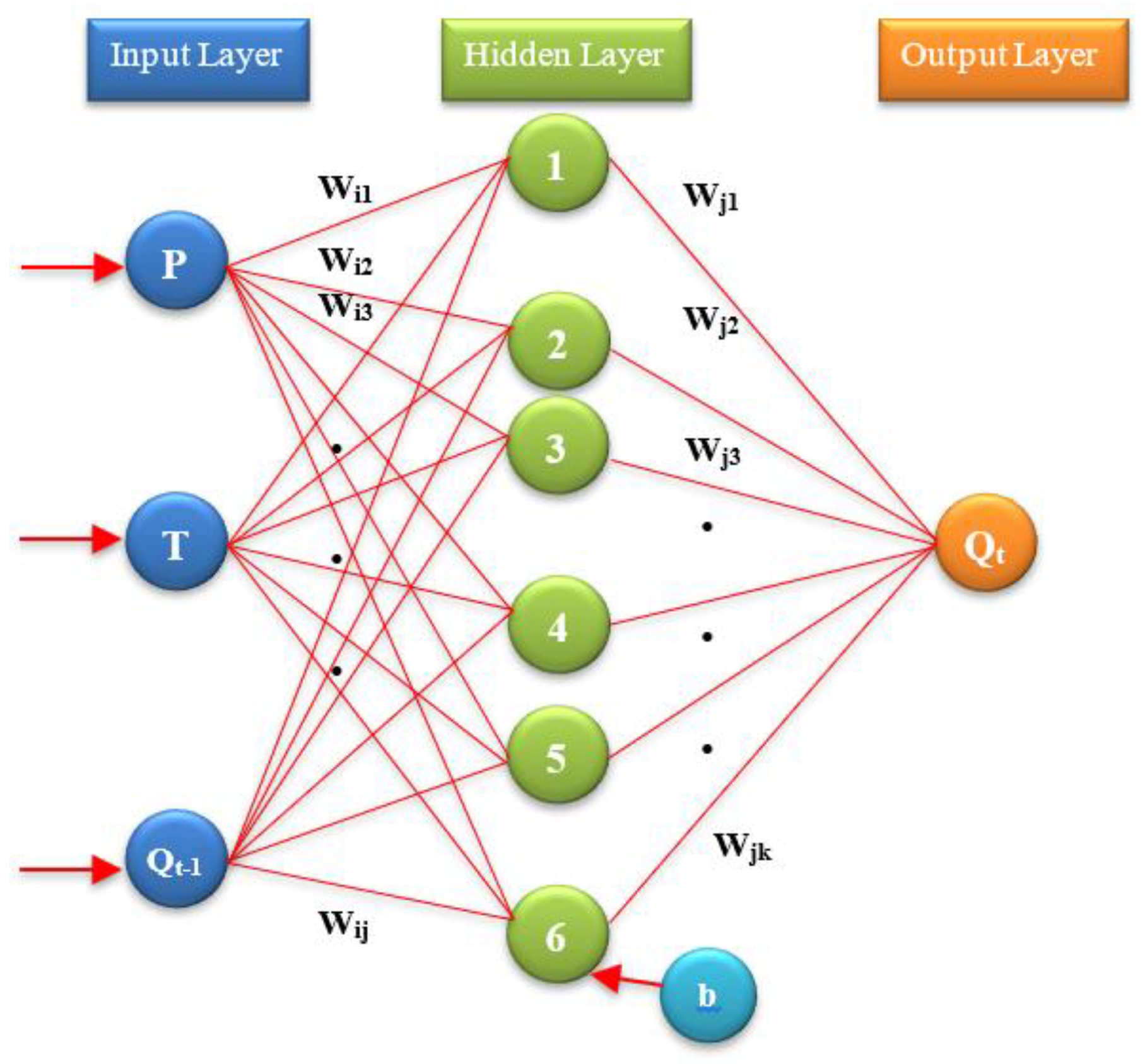
Artificial neural networks (ANN) are systems consisting of process elements that are connected to each other with different weights that are inspired by the structure of nerve cells in the human brain. Among the artificial neural network (ANN) methods, the most commonly used method is the feed-forward back-propagation ANN model, which operates according to the principle of back propagation of errors. An artificial neural network cell consists of five main parts: the input layer, variable weight multipliers, total function, activation function, and output layer. In Figure 3, a schematic diagram of a three-layer artificial neural network is given. According to Figure 3, the river flow time series (Qt − 1), water temperature (Tt) and Precipitation (Pt) were used to estimate the river flow (Qt). The time series is used for estimating the river flow in dry periods when there is no rain affecting the river basin.
In Figure 3, Wij and Wjk, respectively, represent the weight of the connection between the input, hidden and output layers, and “b” is the bias term. Output estimation values for ANN are obtained by adding the bias multiplied by the input values and weighted averages (w). These values are coefficient values that express the effect of the previous input data on the treated element. These coefficients, which initially receive random weight values, constantly vary during the training phase by comparing the predictive outputs to the actual outputs, and the error amounts are propagated backward until the link weight values are adjusted to minimize errors. In this study, the feedback propagation ANN method was used. The technique updates the weights and bias values according to the Levenberg–Marquardt optimization. It minimizes a combination of squared errors and weights, and then determines. As a transfer function; “tansig” was used for the hidden layer, “purelin” was used for the output layer and “trainlm” was used for Back-propagation network training. In addition, the number of epochs was 1000, the momentum coefficient was 0.80, and the learning rate refresh coefficient was 1.15. The ANN model consisted of 3 inputs, 1 hidden layer with 6 nodes, and 1 output layer (Figure 3).

2.2.3. M5 Decision Tree Model (M5T)

Decision trees are a tree-shaped decision structure type whose classes are learned by using the induction method from the sample data. A decision tree is a structure used by applying simple decision steps, dividing large amounts of records into very small groups of records. With each successful division operation, members of the result groups become much more similar to each other. Decision trees are a useful solution in many classification problems using complex databases and in complex or erroneous information. Decision trees, which have predictive and descriptive features, are the most widely used technique among the classification models due to their easy installation, easy interpretation, easy integration into database systems, and their better reliability. The dividing criterion is based on the standard deviation of the subset values. The mathematical formula for calculating standard deviation reduction (SDR) is:
SDR = SD ( T ) T i T × SD ( T i )
In Equation (2), T represents a group of samples reaching the node, Ti represents a subset of samples that are the result of the potential cluster, and SD represents the standard deviation. After examining all possible structures, a structure that has the maximum expected error reduction would be picked out. This dividing process often creates a great tree-like structure that leads to an overfit structure. A general M5 tree is given in Figure 4.

2.2.4. Mamdani Fuzzy Logic (M-FL) Model

The Mamdani system was first studied (Mamdani and Assilian, [32]) in 1975. This system is characterized as very convenient due to its proximity to human behavior among fuzzy logic modeling systems. It is the ancestor of all fuzzy logic models. Its simplicity in modeling has expanded the use of the Mamdani system. It has been used to try to facilitate the solution of the problems through verbal expression, thanks to the fuzzy logic of the models that are not fully known numerically or that have mixed equations. Fuzzy inference is how input or input groups are associated with an output using the fuzzy logic method.
In fuzzy logic models, connections between inputs and outputs are provided using rules in the rule base. A fuzzy logic controller consists of three basic parts: fuzzification, a rule-based extraction mechanism, and defuzzification. A typical example of a “Mamdani-Fuzzy Logic” starts as follows. Input parameters are created for model analysis and the fuzzification process is started. Fuzzy sets ranging from 0–1 are created for each input parameter. These clusters can have different shapes such as triangle, trapezoidal or curvilinear. Then, with our input–output parameters, rules such as fuzzy “If-Then rules” are created. It rinses with the rinsing process, digitizing our fuzzy data and printing. The flow chart of all these processes is shown in Figure 5.
There are two fuzzy inference systems most commonly known in the literature. These inferences are Mamdani and Takagi–Sugeno (Adaptive Neuro-Fuzzy Inference System, ANFIS). Mamdani’s fuzzy inference method is the most commonly used fuzzy method. The Mamdani inference system takes output membership functions as fuzzy sets. A fuzzy set occurs for each output. Fuzzification is indispensable for achieving precise results. This approach is suitable for verbal expressions and when there is not a lot of data. In contrast to Mamdani, the ANFIS (Takagi–Sugeno, [33]) approach uses only numerical data and verbal data cannot be entered. From this point, the ANFIS approach is a data-driven method and gives better results when digital input–output data is provided. ANFIS operates according to the “If-Then” rule and the structure uses the Sugeno fuzzy rules. According to the “if-Then” rule, if x is A1, y is B1; where A1 and B1 are linguistic values defined by fuzzy sets. It is possible to introduce fuzzy systems with logical models consisting of “If-Then” membership rules and membership functions.
Mamdani inference is known as the first control system established by the fuzzy set theory. Mamdani was able to control the combination of the steam engine and boiler by reviewing a set of linguistic control rules found by professional human operators (Mamdani, [34]). His work was based on Zadeh’s study (Zadeh, [9]) on complex systems and fuzzy algorithms for decision-making. The inference process is different from Zadeh’s work, but the basic idea is the same (MathWorks, [35]). Due to Mamdani and Assilian, [32] the first inference method is the most common in practice and literature. To understand the Mamdani structure, we consider a simple two-rule system, where each rule contains two premises and one conclusion. This is similar to a fuzzy system with a double input and a single output. A fuzzy system with two inputs, x1 and x2 (premise), and a single output, y (as a result), is explained by a collection of linguistic IF-THEN proposals in Mamdani form:
IF   x 1   is   A 1 n   and   x 2   is   A 2 n   THEN   y 1   is   B 1 n ,   for   n   =   1 ,   2 ,   ,
where A 1 n   and A 2 n   are the fuzzy sets representing the kth antecedent pairs and   B 1 n is the fuzzy set representing the consequent. In this study, 3 different “LOW”, “MEDIUM” and “HIGH” subsets were determined separately for the water temperature, precipitation, and flow parameters according to Figure 6 and the following rules were created.
IF   T e m p e r a t u r e   is   L O W   and   P r e c i p i t a t i o n   is   MEDIUM   THEN   F l o w   is   HIGH
In Mamdani inference, the result of the “if-Then” rule is defined by a fuzzy set. The fuzzy output set of each rule is reshaped by a matching number in the system, and all of the fuzzy sets obtained as a result of this reshaping must be collected and then rinsed (Wang, [35]). Mamdani Fuzzy Logic has advantages such as proximity to intuitive human perception and logic (MathWorks, [36]). Mamdani’s advantage over Sugeno’s works is to expand Mamdani’s current model, that is, the multi-output model [37].
According to Figure 6, triangular membership functions are used for water temperature, precipitation and flow. The fuzzy subset was tried and determined separately.

2.2.5. Adaptive Neuro-Fuzzy Inference System (ANFIS) Model

This method, also known as the Sugeno type Fuzzy system, consists of a combination of the fuzzy inference system (FIS) and artificial neural networks (ANN). ANFIS systems are the same as Mamdani type fuzzy systems and there are differences in the output result system.
Numerical data cannot be found directly after the output unit of fuzzy systems. The inability to obtain numerical data as a result of fuzzy systems makes it difficult to use the systems from an engineering point of view. Since the printouts are fuzzied in their original form, they cannot be used directly in engineering models. Various studies have been carried out by Takagi and Sugeno [33] and Sugeno–Kank [38] in order to use the fuzzy systems in the equations established with Aristotle’s logic. Figure 7 shows the Takagi–Sugeno–Kank model.
In the Takagi–Sugeno–Kank system, the entrance and fuzzification steps are the same as the Mamdani system. The difference is observed in the output functions. The output functions in this system are fixed or linear. One output data is obtained for each rule. This system is very suitable for mathematical analysis, but it has been observed that it is more unsuccessful than Mamdani in showing an affinity to human behavior.

2.2.6. Simple Membership Functions and Fuzzy Rules Generation Technique (SMRGT)

For the SMRGT method, firstly, dependent and independent variables are determined. In this study, the determination of dependent variables, such as air temperature, precipitation, and the flow variable, was attempted. The minimum and maximum upper limits of these variables were determined and fuzzy clusters (high, medium, low) were determined accordingly. Shapes of the membership functions (triangle, trapeze) were decided. Triangular membership functions are generally preferred in the literature. Then, by determining the unit width, core, and key values of each triangle membership function, membership function processes are completed. During the training process, fuzzy rules are created for each parameter and the process of getting results is started. The flow chart of SMRGT is represented in Figure 8. Researchers can examine more information about SMRGT in Altaş et al. [39], Toprak [40] and Toprak et al. [41,42] ‘s works.
For the prediction model, the unit width (UW), core value (Ci), and key values (Ki) of the fuzzy sets were determined (Figure 9). In order to determine these values, the change interval (VR) of the metrics must be known first. The lowest and highest values of the metrics specified in the second stage were used to determine the change interval. Equation (5) shows the change interval (VR) formula. The parameters used to create membership functions are calculated by the following equations [39,40,41].
V R = ( T , P , Q ) max ( T , P , Q ) min
C i = V R 2 ( T , P , Q ) min
In this paper, calculations were made for minimum and maximum values in the training process for Temperature (T), Rainfall (P) and Flow (Q) values. The nu value used in these equations indicates the total number of right triangles. According to Figure 9, there are two right triangle membership functions in the sides and 2 in the middle (1 isosceles triangle). Calculations for UW, O, EUW, K1, K2 values were performed with the Equations (7)–(11) below.
UW = V R n u
O = UW 2
EUW = V R n u + O
K 1 = ( T , P , Q ) min + EUW 3
K 2 = ( T , P , Q ) max EUW 3
Equations between (Equations (7) and (11)) were used to construct the SMRGT model 1 with borders of membership function and key values. According to Figure 9, the “K1, K1 + UW, K2-UW and K2” values represent the selected triangle membership/cluster limit values. “UW” indicates the unit width and nu is the number of right-angled triangles. The expanded base width (EUW) is needed to find the “K1, K2” limit values and to prevent neighbouring clusters from being nested. The “O” value is an expression used to find the EUW, K1 and K2 values.
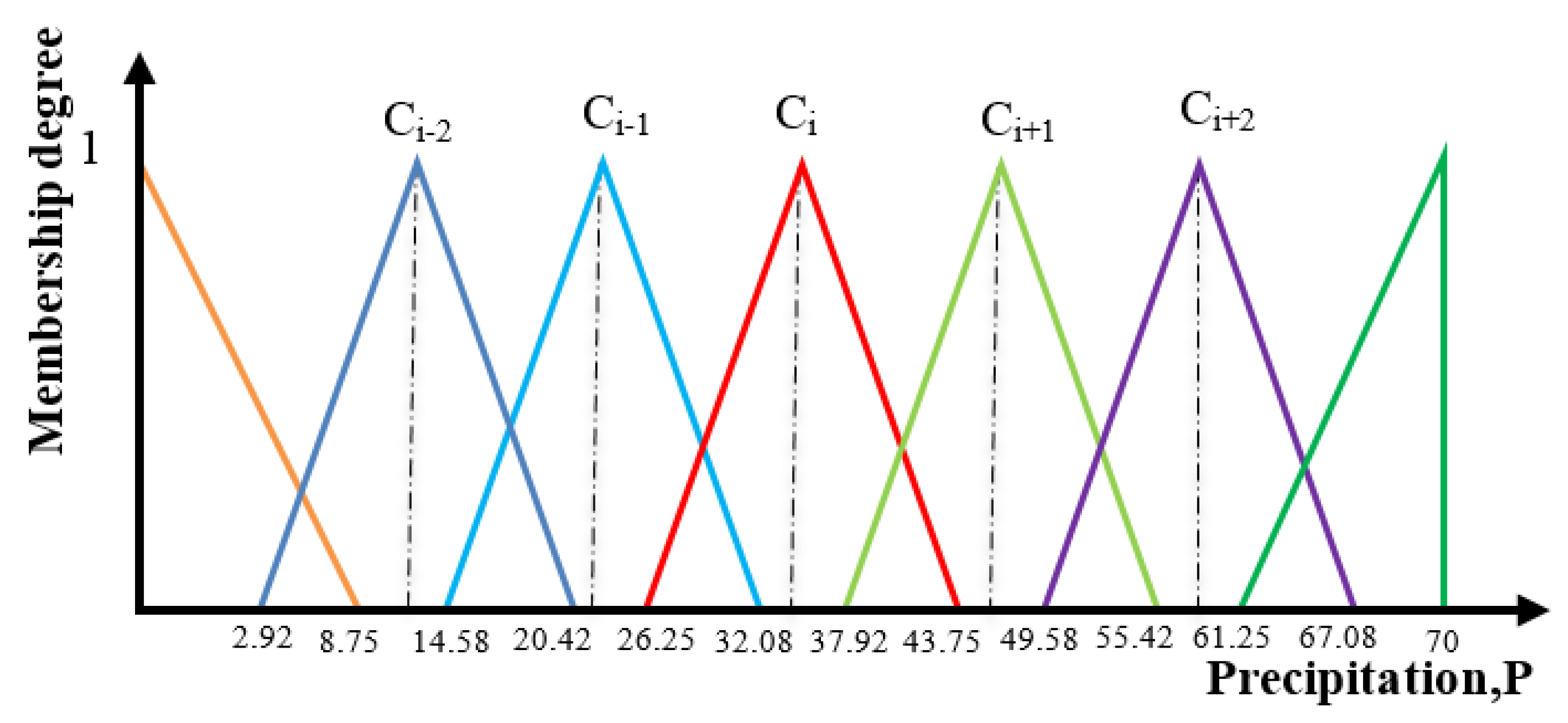
After determining the ranges and structure of the Membership Functions (MFs), the functions of the SMRGT model are given in Figure 10, Figure 11 and Figure 12.
For the SMRGT method, 7 subset membership functions were selected. It was observed that the number of errors decreased as the number of memberships increased. In the SMRGT method, the limit values (Figure 10, Figure 11 and Figure 12) were calculated manually.
Essentially, the SMRGT model is also made with the fuzzy-Mamdani technique. However, fuzzy sub-sets are chosen randomly with the conscientious technique and this makes modeling and model education difficult. However, in the SMRGT model, the fuzzy subset and variable ranges are selected based on observations and experiences. This approach technique makes it easier and more convenient to reflect the physics of the event to the fuzzy model.

3. Results and Discussion

In this study, the flow rate in the river was estimated by using artificial intelligence techniques and Multi Linear Regression methods. The results were compared with each other. A total of 1095 data belonging to the years 2014–2017 were used in the station. Overall, 75% of all data was used for training and 25% was used for the testing. Daily Temperature (Tt), precipitation (Pt) and lagged day flow rate (Qt − 1) were used for estimating the flow (Qt) in the river. In all models, 820 data were trained and 275 data were applied during the test phase.
In order to determine the success of the models used to estimate the flow value in the river, MSE (square error) MAE (mean absolute error) and R (correlation coefficient), given in Equation (12) [43] and Equation (13) [44], were used. Here n represents the number of data for the flow amounts of Q.
MSE = 1 n i = 1 n ( Q observation Q prediction ) 2
MAE = 1 n i = 1 n | Q observation Q prediction |
The performance of the model results is shown in Table 1. When Table 1 was examined, all models gave similar results. According to the MSE, MAE, and R criteria, the best results were obtained in the M-FL and SMRGT models. The M5T models gave the worst results in all criteria.
Daily water Temperature (Tt), Precipitation (Pt) and lagged day flow rate (Qt − 1) were used for MLR flow (Qt) estimations. The MLR model established using training data is given in Equation (14). This equation was also applied to test data.
Q t = 0.2959 0.0146   × T t + 0.0277 ×   P t + 0.8067 ×   Q t     1
MLR model variation and scatter graphs are given in Figure 13. When scatter graphs for testing data were analyzed, the correlation coefficient was obtained as R: 0.902 and MLR values were seen to be close to the actual values.
Feedback propagation network is used for ANN. ANN model results for flow estimation are given in Figure 14. When the variation graph in Figure 14 was examined, it was seen that the measurement and estimation results were similar to each other as in the other models. When the scatter graph in Figure 14 was examined, it was seen that the correlation coefficient was 0.907.
The variation and scatter graphs of M5 decision tree (M5T) model results are given in Figure 15. When the graphs were examined, it was seen that there was a good correlation between the measurement results and the estimation results. Although the correlation coefficient was R: 0.878, it showed the worst performance with the lowest correlation among all models.
In ANFIS analysis, Gaussian parabolic 3 × 3 × 3 Membership Functions (MFs) and Grid partition section were analyzed with 100 iterations, assuming the output as linear. Variation and scatter graphs for the ANFIS method are shown in Figure 16. The correlation coefficient is seen as R: 0.903 in Figure 16. As seen in the figure, ANFIS results were close to the observed values. As shown in Table 1, ANFIS and MLR methods had similar correlations (R: 0.902). When we look at the MSE and MAE criteria, they have similar low error rates.
The scatter and variation graphs of the M-FL method are shown in Figure 17. When the variation graph was examined, it was seen that the predicted values gave closer results to the actual values. The scatter diagram also shows a high correlation between the actual values and the estimated values. Compared to all models, it can be seen from Table 1 that M-FL model results have lower error rates (MSE: 0.595; MAE: 0.338) and higher correlation (R: 0.917)
Simple Membership Functions and Fuzzy Rules Generation Technique (SMRGT) model results for flow estimation are given in Figure 18. When the variation graph in Figure 18 was examined, it was seen that the predicted values gave closer results to the actual values. When the scatter graph in Figure 18 was examined, it was seen that the correlation coefficient was 0.927. In Table 1, it was found that the SMRGT model showed the best performance among all models followed by the M-FL model. Compared to all models, it can be seen from Table 1 that SMRGT model results had the lowest error rates (MSE: 0.535; MAE: 0.318) and the highest correlation (R: 0.927).
As is known, ANN, M5 Tree and ANFIS models are black-box models. They cannot adequately consider the physics of the event between input and output. However, the Fuzzy Mamdani and SMRGT models presented in this study offer the opportunity to reflect the physics of the event to the model using measurement changes, experience, and knowledge. It was observed that the 275 data used in the testing of the models did not reach the flow peak values in all models at approximately five extraordinary flood flow rates. Therefore, it was observed that the correlation values decreased.

4. Conclusions

In this study, daily average water temperature, precipitation, and lagged day flow values were used for flow prediction. A total of 1095 daily data belonging to the year range of 2014–2017 in Worcester county of Sterling region, USA were examined. Flow in the river was estimated by using Multi Linear Regression (MLR), Artificial Neural Network (ANN), M5 Decision Tree (M5T), Adaptive Neuro-Fuzzy Inference System (ANFIS), Mamdani-Fuzzy Logic (M-FL) and Simple Membership Functions and Fuzzy Rules Generation Technique (SMRGT) models. The best models were found by applying statistical indicators such as MSE, MAE, and R. The results obtained in this paper are given below.
  • The SMRGT model shows the best statistical performance compared to the other models. (MSE: 0.535 m6/s2, MAE: 0.318 m3/s and R: 0.927).
  • The M-FL model exhibits a better performance (MSE: 0.595 m6/s2, MAE: 0.338 m3/s and R: 0.917) than the ANN, ANFIS, M5T and MLR models.
  • The MLR and ANFIS models have nearly the same results. For MLR, MSE: 0.618 m6/s2, MAE: 0.347 m3/s and R: 0.902. For the ANFIS model, MSE: 0.611 m6/s2, MAE: 0.345 m3/s and R: 0.903.
  • The ANN method gives better results than the MLR, ANFIS and M5T methods (MSE: 0.601 m6/s2, MAE: 0.349 m3/s and R: 0.907).
  • The M5T method shows the lowest performance among all models (MSE: 0.747 m6/s2, MAE: 0.370 m3/s and R: 0.878).
According to the MSE, MAE, and R criteria, the worst results were obtained in the M5T model. The MLR, ANN, and ANFIS results were closer to each other. The best results were obtained in the M-FL and SMRGT models. Compared to all models, the SMRGT model results had the lowest error rates and the highest correlation. As a result of this study, the SMRGT methods are recommended for future hydrological and water resources analysis.
The rainfall flow relationship is a multivariate nonlinear event. For this reason, it is very difficult to accurately determine all parameters, and parametric modeling of precipitation-flow relationship. The new artificial intelligence techniques in the presented study are thought to be used in determining the relationship between precipitation flow depending on past seasonal parameters.

Author Contributions

Conceptualization, F.Ü. and M.D.; methodology, M.Z.; software, F.Ü. and B.T.; validation, M.Ç.; formal analysis, M.Z.; investigation, M.Ç.; resources, M.D.; data curation, Y.Z.K.; writing—original draft preparation, F.Ü.; writing—review and editing, Y.Z.K., F.V. and M.Z.; visualization, B.T. All authors have read and agreed to the published version of the manuscript.

Funding

This work was supported by the project of the Ministry of Education of the Slovak Republic VEGA 1/0308/20: Mitigation of hydrological hazards—floods and droughts—by exploring extreme hydroclimatic phenomena in river basins and the project of the Slovak Research and Development Agency APVV-18-0360: Active hybrid infrastructure towards a sponge city.

Acknowledgments

The authors would like to thank to U.S. Geological Survey for their effort on measurement of the data used in this study and for their open access data policy.

Conflicts of Interest

The authors declare no conflict of interest.

References

  1. Hsu, K.L.; Gupta, H.V.; Sorooshian, S. Artificial neural network modeling of the rainfall-runoff process. Water Resour. Res. 1995, 31, 2517–2530. [Google Scholar] [CrossRef]
  2. Fernando, D.A.K.; Jayawardena, A.W. Runoff forecasting using RBF networks with OLS algorithm. J. Hydrol. Eng. 1998, 3, 203–209. [Google Scholar] [CrossRef]
  3. Tokar, A.S.; Johnson, P.A. Rainfall-runoff modeling using artificial neural networks. J. Hydrol. Eng. 1999, 4, 232–239. [Google Scholar] [CrossRef]
  4. Sinha, J.; Sahu, R.K.; Agarwal, A.; Pali, A.K.; Sinha, B.L. Rainfall-Runoff Modelling using Multi Layer Perceptron Technique—A Case Study of the upper Kharun Catchment in Chhattisgarh. J. Agric. Eng. 2013, 50, 43–51. [Google Scholar]
  5. Sivakumar, B.; Jayawardena, A.W.; Fernando, T.M.K.G. River flow forecasting: Use of phase-space reconstruction and artificial neural networks approaches. J. Hydrol. 2002, 265, 225–245. [Google Scholar] [CrossRef]
  6. Jain, S.K.; Das, A.; Srivastava, D.K. Application of ANN for reservoir inflow prediction and operation. J. Water Resour. Plan. Manag. 1999, 125, 263–271. [Google Scholar] [CrossRef]
  7. Raghuwanshi, N.S.; Singh, R.; Reddy, L.S. Runoff and Sediment yield modeling using artificial neural networks: Upper Siwane River, India. J. Hydrol. Eng. 2006, 11, 71–79. [Google Scholar] [CrossRef]
  8. Senthil Kumar, A.R.; Ojha, C.S.P.; Goyal, M.K.; Singh, R.D.; Swamee, P.K. Modeling of suspended sediment concentration at Kasol in India using ANN, fuzzy logic, and decision tree algorithms. J. Hydrol. Eng. 2012, 17, 394–404. [Google Scholar] [CrossRef]
  9. Zadeh, L.A. Fuzzy sets. Inf. Control 1965, 8, 338–353. [Google Scholar] [CrossRef] [Green Version]
  10. Nayak, P.C.; Sudheer, K.P.; Ramasastri, K.S. Fuzzy computing based rainfall–runoff model for real time flood forecasting. Hydrol. Process. 2005, 19, 955–968. [Google Scholar] [CrossRef]
  11. Mamdani, E.H.; Assilian, S. An experiment in linguistic synthesis with a fuzzy logic controller. Int. J. Hum. Comput. Stud. 1999, 51, 135–147. [Google Scholar] [CrossRef]
  12. Gowda, C.C.; Moyya, S.D. Runoff modelling using different membership functions in adaptive neuro fuzzy inference system. Int. J. Eng. Sci. 2014, 4, 48–51. [Google Scholar]
  13. Chang, L.C.; Chang, F.J.; Tsai, Y.H. Fuzzy exemplar-based inference system for flood forecasting. Water Resour. Res. 2005, 41, 1–12. [Google Scholar] [CrossRef]
  14. Maskey, S.; Guinot, V.; Price, R.K. Treatment of precipitation uncertainty in rainfall-runoff modelling: A fuzzy set approach. Adv. Water Resour. 2004, 27, 889–898. [Google Scholar] [CrossRef]
  15. Tayfur, G.; Moramarco, T.; Singh, V.P. Predicting and forecasting flow discharge at sites receiving significant lateral inflow. Hydrol. Process. 2007, 21, 1848–1859. [Google Scholar] [CrossRef] [Green Version]
  16. Tilmant, A.; Vanclooster, M.; Duckstein, L.; Persoons, E. Comparison of fuzzy and nonfuzzy optimal reservoir operating policies. J. Water Resour. Plan. Manag. 2002, 128, 390–398. [Google Scholar] [CrossRef]
  17. Kocabaş, F.; Ünal, B.; Ünal, S.; Fedakar, H.I.; Gemici, E. Fuzzy genetic approach for modeling of the critical submergence of an intake. Neural Comput. Appl. 2013, 23, 73–82. [Google Scholar] [CrossRef]
  18. Ozel, H.U.; Gemici, B.T.; Ozel, H.B.; Gemici, E. Determination of Water Quality and Estimation of Monthly Biological Oxygen Demand (BOD) Using by Different Artificial Neural Networks Models. Fresenius Environ. Bull. 2017, 26, 5465–5476. [Google Scholar]
  19. Hong, Y.S.; Rosen, M.R.; Reeves, R.R. Dynamic fuzzy modeling of storm water infiltration in urban fractured aquifers. J. Hydrol. Eng. 2002, 7, 380–391. [Google Scholar] [CrossRef]
  20. Zahiri, A.; Azamathulla, H.M. Comparison between linear genetic programming and M5 tree models to predict flow discharge in compound channels. Neural Comput. Appl. 2014, 24, 413–420. [Google Scholar] [CrossRef]
  21. Sattari, M.T.; Pal, M.; Apaydin, H.; Ozturk, F. M5 model tree application in daily river flow forecasting in Sohu Stream, Turkey. Water Resour. 2013, 40, 233–242. [Google Scholar] [CrossRef]
  22. Singh, K.K.; Pal, M.; Singh, V.P. Estimation of mean annual flood in Indian catchments using backpropagation neural network and M5 model tree. Water Resour. Manag. 2010, 24, 2007–2019. [Google Scholar] [CrossRef]
  23. Kisi, O.; Khosravinia, P.; Nikpour, M.R.; Sanikhani, H. Hydrodynamics of river-channel confluence: Toward modeling separation zone using GEP, MARS, M5 Tree and DENFIS techniques. Stoch. Environ. Res. Risk Assess. 2019, 33, 1089–1107. [Google Scholar] [CrossRef]
  24. Al-Abadi, A.M. Modeling of stage–discharge relationship for Gharraf River, southern Iraq using backpropagation artificial neural networks, M5 decision trees, and Takagi–Sugeno inference system technique: A comparative study. Appl. Water Sci. 2016, 6, 407–420. [Google Scholar] [CrossRef] [Green Version]
  25. Shaghaghi, S.; Bonakdari, H.; Gholami, A.; Kisi, O.; Binns, A.; Gharabaghi, B. Predicting the geometry of regime rivers using M5 model tree, multivariate adaptive regression splines and least square support vector regression methods. Int. J. River Basin Manag. 2019, 17, 333–352. [Google Scholar] [CrossRef]
  26. Demirci, M.; Baltaci, A. Prediction of suspended sediment in river using fuzzy logic and multilinear regression approaches. Neural Comput. Appl. 2013, 23, 145–151. [Google Scholar] [CrossRef]
  27. Demirci, M.; Üneş, F.; Saydemir, S. Suspended sediment estimation using an artificial intelligence approach. In Sediment Matters; Springer: Cham, Switzerland, 2015; pp. 83–95. [Google Scholar]
  28. Üneş, F.; Demirci, M.; Kişi, Ö. Prediction of millers ferry dam reservoir level in USA using artificial neural network. Period. Polytech. Civ. Eng. 2015, 59, 309–318. [Google Scholar] [CrossRef]
  29. Üneş, F.; Demirci, M.; Ispir, E.; Kaya, Y.Z.; Mamak, M.; Tasar, B. Estimation of Groundwater Level Using Artificial Neural Networks: A Case Study of Hatay-Turkey. In Proceedings of the 10th International Conference “Environmental Engineering”, Vilnius Gediminas Technical University, Vilnius, Lithuania, 27–28 April 2017; Volume 10, pp. 1–6. [Google Scholar]
  30. Demirci, M.; Unes, F.; Kaya, Y.Z.; Tasar, B.; Varcin, H. Modeling of Dam Reservoir Volume Using Adaptive Neuro Fuzzy Method. In Proceedings of the Air and Water Components of the Environment Conference, Sovata, Romania, 15–17 March 2018; pp. 145–152. [Google Scholar] [CrossRef] [Green Version]
  31. USGS.gov | Science for a Changing World [WWW Document]. Available online: https://www.usgs.gov/ (accessed on 20 May 2019).
  32. Mamdani, E.H. Advances in the linguistic synthesis of fuzzy controllers. Int. J. Man-Machine Stud. 1976, 8, 669–678. [Google Scholar] [CrossRef]
  33. Takagi, T.; Sugeno, M. Fuzzy identification of systems and its applications to modeling and control. IEEE Trans. Syst. Man. Cybern. 1985, 1, 116–132. [Google Scholar] [CrossRef]
  34. Mamdani, E.H. Application of fuzzy algorithms for control of simple dynamic plant. Proc. Inst. Electr. Eng. 1974, 121, 1585–1588. [Google Scholar] [CrossRef]
  35. Wang, C. A Study of Membership Functions on Mamdani-Type Fuzzy Inference System for Industrial Decision-Making. Master’s Thesis, Lehigh University, Bethlehem, Pennsylvania, 2015. [Google Scholar]
  36. Math Works. Fuzzy Logic Toolbox, User’s Guide R2014a; The Mathworks Inc.: Natick, MA, USA, 2014. [Google Scholar]
  37. Rodić, D.; Sekulić, M.; Gostimirović, M.; Pucovsky, V.; Kramar, D. Fuzzy logic and sub-clustering approaches to predict main cutting force in high-pressure jet assisted turning. J. Intell. Manuf. 2020, 1–16. [Google Scholar] [CrossRef]
  38. Sugeno, M.; Kank, G.T. Structure identification of fuzzy model. Fuzzy Sets Syst. 1988, 28, 15–33. [Google Scholar] [CrossRef]
  39. Altaş, E.; Aydın, M.C.; Toprak, Z.F. Açık kanal akımlarında su yüzü profilinin bulanık SMRGT yöntemiyle modellenmesi. Dicle Üniv. Mühendis. Fakültesi Mühendis. Derg. 2018, 9, 975–981. [Google Scholar]
  40. Toprak, Z.F. Flow discharge modeling in open canals using a new fuzzy modeling technique (SMRGT). Clean Soil Air Water 2009, 37, 742–752. [Google Scholar] [CrossRef]
  41. Toprak, S.; ATAY, A.; Toprak, Z.F. SMRGT yöntemi ile bulanıklaştırılmış veriler için bulanık doğrusal regresyon. Erciyes Üniv. Fen Bilimleri Enst. Fen Bilimleri Derg. 2015, 31, 1–7. [Google Scholar]
  42. Toprak, A.; Aykaç, Z.; Toprak, Z.F. Bulanık SMRGT yönteminin pratik uygulamaları. Dicle Üniv. Mühendis. Fak. Mühendis. Derg. 2017, 1, 123–132. [Google Scholar]
  43. Willmott, C.J.; Matsuura, K. Advantages of the mean absolute error (MAE) over the root mean square error (RMSE) in assessing average model performance. Clim. Res. 2005, 30, 79–82. [Google Scholar] [CrossRef]
  44. Quan, Q.; Hao, Z.; Xifeng, H.; Jingchun, L. Research on water temperature prediction based on improved support vector regression. Neural Comput. Appl. 2020, 1–10. [Google Scholar] [CrossRef]
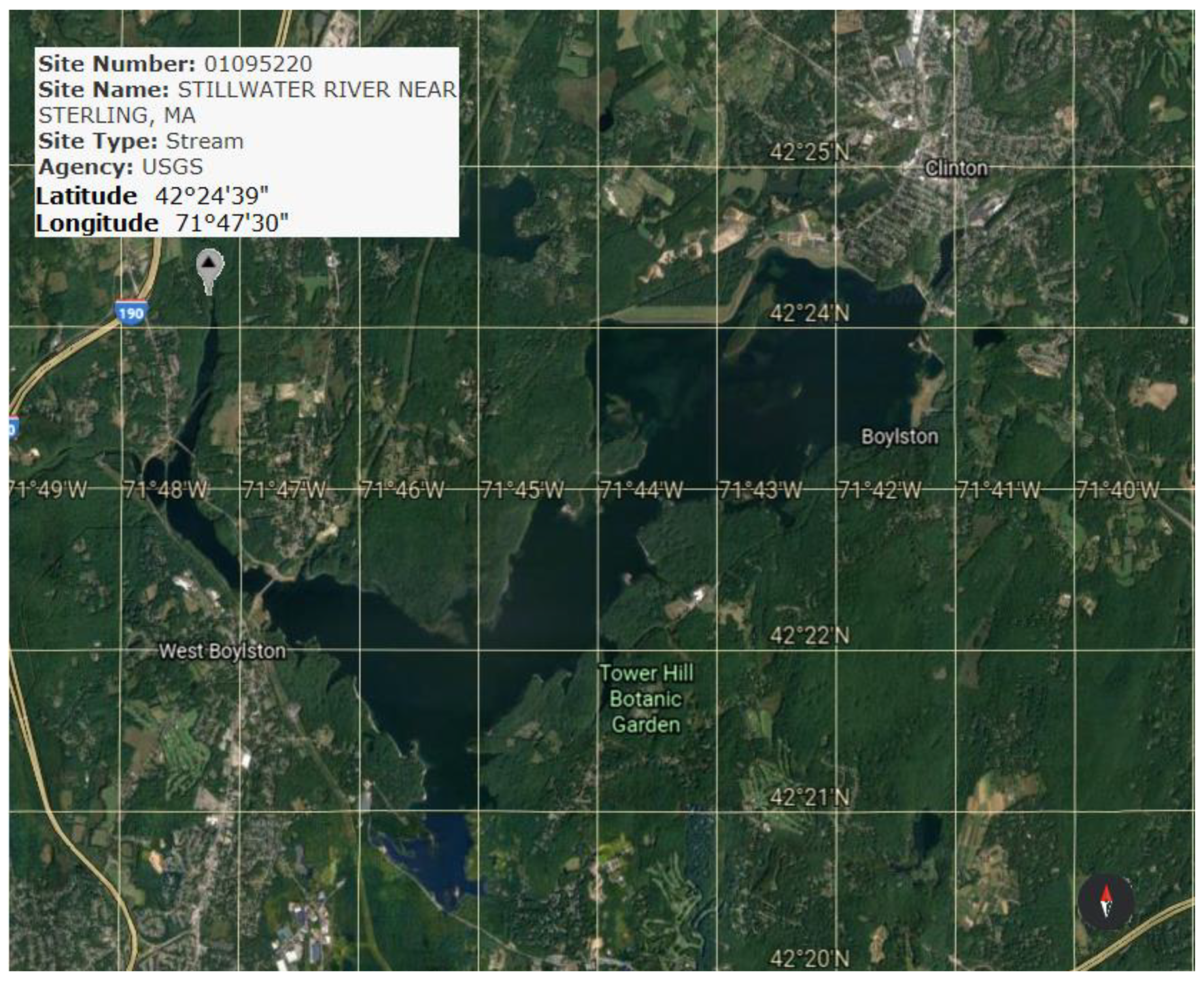
Figure 1. Location of Study Area [31].
Water 12 02427 g001
Figure 2. Stillwater River Discharge changes in the Sterling Region (a) in the rainy season, (b) in the non-rainy season.
Water 12 02427 g002aWater 12 02427 g002b
Figure 3. Schematic diagram of a three-layer ANN that was used in this study.
Water 12 02427 g003
Figure 4. General M5 tree structure.
Water 12 02427 g004
Figure 5. Basic structure of fuzzy logic.
Water 12 02427 g005
Figure 6. The Mamdani Fuzzy Logic MFs plots for (a) water temperature; (b) precipitation; (c) River flow.
Water 12 02427 g006
Figure 7. Takagi–Sugeno–Kank Fuzzy System.
Water 12 02427 g007
Figure 8. Flow chart of SMRGT.
Water 12 02427 g008
Figure 9. Figural representation of unit width, core value, and key values for SMRGT.
Water 12 02427 g009
Figure 10. The SMRGT MFs plots for temperature variables.
Water 12 02427 g010
Figure 11. The SMRGT MFs plots for precipitation variables.
Water 12 02427 g011
Figure 12. The SMRGT MFs plots for flow variables.
Water 12 02427 g012
Figure 13. Observed and MLR model for river flow test data: (a) variation graph, (b) scatter graph.
Water 12 02427 g013aWater 12 02427 g013b
Figure 14. Observed and ANN model for river flow test data: (a) variation graph, (b) scatter graph.
Water 12 02427 g014aWater 12 02427 g014b
Figure 15. Observed and M5T model for river flow test data: (a) variation graph, (b) scatter graph.
Water 12 02427 g015aWater 12 02427 g015b
Figure 16. Observed and ANFIS model for river flow test data: (a) variation graph, (b) scatter graph.
Water 12 02427 g016aWater 12 02427 g016b
Figure 17. Observed and M-FL model for river flow test data: (a) variation graph, (b) scatter graph.
Water 12 02427 g017aWater 12 02427 g017b
Figure 18. Observed and SMRGT model for river flow test data: (a) variation graph, (b) scatter graph.
Water 12 02427 g018aWater 12 02427 g018b
Table 1. MSE, MAE and R parameters for the comparison of model results.
ModelsMSE (m3/s)2MAE (m3/s)R
MLR0.6180.3470.902
ANN0.6010.3490.907
M5T0.7470.3700.878
ANFIS0.6110.3450.903
M-FL0.5950.3380.917
SMRGT-FL0.5350.3180.927
MSE: Mean square error, MAE: mean absolute error, R: correlation coefficient.