Decision-Making of LID-BMPs for Adaptive Water Management at the Boise River Watershed in a Changing Global Environment

Abstract

We conducted a study on water management at the Boise River Watershed in a changing global environment potentially induced by climate variability and urbanization. Environmental ‘hotspots’ associated with water quality and quantity were first identified to select suitable management options, such as Low Impact Development (LID is commonly used for urban storm water management to reduce impacts induced by flash flood in urban environment while improving water quality standard by filtering non-point source pollutants from predominant, impervious land segments in urban settings.) and Best Management Practices (BMPs) for urban and rural land segments, respectively. A decision-making process was employed to evaluate the cost-effectiveness for each management option based on multiple criteria, including water quality, financial challenges, and other environmental concerns. The results show that LID/BMPs were useful to control water quality in the watershed. The effectiveness of LID/BMPs implementation was subject to change with the placement location and consideration objectives associated with economic or environmental aspects. It appears that about 10% of the study area is required to implement water management options (LID/BMP) to improve water quality potentially driven by climate variability and urbanization. We anticipate that this study will make a case toward developing a sustainable water management plan in a changing global environment, especially for the urban–rural interface settings.

1. Introduction

Water quality is one of the significant environmental issues at the urban–rural interface, such as Boise in the United States (US) [1]. Changing the global environment driven by climate variability, urbanization, and population growth further affects water quality standards across the states. Nutrient loadings from urban runoffs and agricultural return flows create taste and order problems and disrupt recreation activities [2,3]. Population growth and economic development overexploit surface and groundwater resources [4,5], yet it is challenging to manage water resources due to the complicated nature and human dynamics. Exploring adaptive water management, therefore, is a critical exercise to mitigate water quality (WQ) impacts in this changing global environment. Adaptive water management represents systematic processes to improve water management practices and policies by recognition of the importance of the human and social dimensions of resource use.

Two typical approaches, including Low Impact Development (LID) and Best Management Practice (BMP), are used to mitigate WQ impacts for the urban and rural settings, respectively. Although the terms of LID and BMP (LID/BMP) are often used interchangeably and widely implemented at the urban–rural interface, the pollutant removal efficiency (e.g., sediment, total phosphorus, and total nitrogen) varies depending on their configuration and installation locations [6]. The identification of the critical hotspot (CHS), therefore, is a necessary step to apply an appropriate LID and/or BMP choice at their respective sub-watershed. Traditionally, hydrological models and decision-making tools are commonly used to identify CHSs in the field of water management practices [7,8,9]. Thus, Ref. [10] applied the Soil and Water Assessment Tool (SWAT) model to identify CHSs in the Rock River watershed in Vermont, while [11] used a decision support system to select BMP options with the identified CHSs.

Once CHSs are identified, additional effort is needed to select the proper LID and/or BMP choice. Basically, the multi-criteria decision analysis (MCDA) is a useful tool for this purpose in the sense that it can provide the unique and systematic processes for the various decision-makers [12,13,14,15]. The MCDA incorporates a rich collection of techniques and procedures for structuring decision problems, designing, evaluating, and prioritizing alternatives on decisions, but the decision-making procedure tends to rely on personal experiences and choice as they apply an MCDA method to see fit. Ref. [16] suggested the four main types of decision procedures using the MCDA method. The first category is (1) the choice problem to select the single optimal option. The second category is (2) the sorting problem. Thus, several alternatives are sorted to regroup alternatives with similar behavior based on features indicating clear, organizational, or predictive reasons. The third category is (3) the ranking problem. The alternatives are re-ordered from the best to the worst by means of scores or pairwise comparisons. The last category is (4) the description problem, which elaborates alternatives and consequences during the process.

Later, more studies have been conducted to evaluate alternatives using an optimization approach within MCDA [17,18,19,20]; Ref. [21] created a new method for optimizing pairwise comparison decision-making matrices in MCDA to apply land subsidence susceptibility mapping. Ref. [22] developed an optimization model to identify geographic priorities for groundwater management by minimizing operational costs. Ref. [23] also applied an optimization method to explore land management by maximizing net profits and by minimizing erosion risks. Ref. [24] integrated the Qual2k model and a multi-objective evolutionary algorithm (MOEA) to select the adequate treatment type for wastewater treatment plants to improve water quality at river basin scales.

It needs to evaluate localized site scale benefits and cumulative effects on the implementation of LID/BMPs across the selected hotspots in changing the global environment using multi-objective decision analysis. However, a few studies have been conducted to select optimal LID/BMP of implementation from many available types of how to define the cost-effectiveness and strategy possibility of water management by the hotspots, especially in a changing future climate and land use. In this study, we explored adaptive water management at the study area in a changing global environment with the following steps based on our previous studies. First, we used the MCDA approach to select the best LID/BMP choice in consideration of multiple criteria, including water quality, economic feasibility, and other environmental concerns associated with climate variability and urbanization. Hydrological simulations with climate inputs were also conducted to assess water quality and quantity (WQQ) in the study area. Next, we evaluated the selected LID/BMP to explore water management alternatives by mitigating water quality impacts. Lastly, we briefly address the result outcomes and future work. This study will strengthen science-based decision-making for adaptive water management and provide useful insight to policy-makers for cost-effective water management decisions.

2. Materials and Methods

2.1. Study Area

The Boise River Watershed (BRW) was selected for the study area (Figure 1). The BRW is 10,439 km² with a mainstream length of a 164 km stretch and flows into the Snake River near Parma. The mean annual rainfall in this watershed is 274 mm, and the average annual temperature has been 13.70 °C from 1979 to 2016. More than 40% of Idaho’s population lives in the greater Boise metropolitan areas, including Boise, Nampa, Meridian, and Caldwell. Concerns of water quality degradation, however, have been discussed in the scientific communities due to recent urbanization and climate variability.

2.2. Hydrological Simulation Program–Fortran (HSPF) Model

For a hydrological model, the Hydrological Simulation Program–Fortran (HSPF) from the previous work [25] was selected and applied for this study. HSPF is a watershed scale, process-based, and semi-distributed model. This model can effectively simulate streamflow and water quality associated with land management practices and climate variability at the urban–rural interface, such as BRW [26,27,28,29,30]. The HSPF model consists of the main three modules (PERLND, IMPLND, and RCHERS). Each module has different parameter sets for hydrology, water quality components, and state variables [31]. For HSPF model evaluation, Nash-Sutcliffe Efficiency (NSE), correlation coefficient (R), Mean Square Error-observation standard deviation ratio (RSR), and percentage of bias (PBIAS) are computed for model calibration and validation (see Appendix A).

2.3. Data Used

2.3.1. Meteorological Data

Phase 2 of the North American Land Data Assimilation System (NLDAS-2) data was used to retrieve climate forcing data, including precipitation, temperature, wind speed, solar radiation. The NLDAS-2 is available from the hourly to yearly time step with 1/8th-degree grid spacing for the simulation period from 1 January 1979 to 31 December 2015. Cloud cover data, however, were derived separately from Climate Data Online (CDO) provided by the National Climatic Data Center (NCDC), because they are not included in NLDAS-2. Dew-point data, T_dew, are also calculated separately using an empirical equation [32] based on grid points of NLDAS-2 within the BRW.

$$PET= \frac{0.408\Delta \left(R_n-G\right)+\gamma \frac{900}{T+273}{u}_2\left(e_s-e_a\right)}{\Delta +\gamma \left(1+0.34u_2\right)}$$

(1)

where PET = Penman–Monteith Potential Evapotranspiration Estimate, Rn = net radiation at the crop surface (MJ/m²/day), G = soil heat flux density (MJ/m²/day), T = mean daily air temperature (°C), u₂ = wind speed at 2 m height (m/s), e_s = saturation vapor pressure (kPa), e_a = actual vapor pressure (kPa), Δ = slope vapor pressure curve (kPa/°C), γ = psychrometric constant (kPa/°C).

The derived and calculated data from NLDAS-2 (112 grid points for BRW) are aggregated for each sub-watershed to compute mean areal values, and then they are routed into HSPF.

$$T_{dew}= \frac{T}{\left[\frac{m}{{\log }_{10}\left(\frac{P_{ws}}{A}\right)}-1\right]}$$

(2)

$$P_{ws}=A \times {10}^{\left[\frac{m\times T}{T+T_n}\right]}$$

(3)

where T_dew is calculated dew point (°C), T is air temperature (°C), A, m, and T_n are constants as referred to [32]. P_ws is water vapor saturation pressure over water (hPa). Penman–Monteith’s equation below [33] is used to compute PET.

2.3.2. Hydrological Data

Observed daily streamflow for 1981–2015 was used to calibrate (2001–2015) and validate (1981–2000) for HSPF. A total of 6 observed streamflow stations were selected as calibration target points including 3 points above reservoirs, 2 points below reservoirs, and 1 point at the watershed outlet, as shown in Figure 1. Water quality calibration was conducted for sediment, total nitrogen (TN), and total phosphorus (TP) at the watershed outlet. Since there are not enough observed daily water quality data, adequate efforts for manual calibrations were made to estimate optimal model parameters for water quality simulations.

Table 1. Streamflow and water quality parameters used for model calibration at the BRW.

Parameter	Definition	Units	Initial Value	Possible Range of Values	Calibrated Value
AGWETP 1	Fraction of remaining potential evapotranspiration from active groundwater	None	0	0–1.0	0.003
AGWRC 1	Base groundwater recession rate	None	0.98	0.82–0.999	0.96
BASETP 1	Fraction of potential evapotranspiration from baseflow	None	0.02	0–1.0	0.14
CEPSC 1	Interception storage capacity	mm	2.54	0.25–254	10.32
DEEPFR 1	Fraction of groundwater inflow to deep recharge	None	0.1	0.0–1.0	0.41
INFILT 1	Infiltration rate	mm/h	4.06	0.03–12.70	2.33
INTFW 1	Interflow inflow parameter	None	2.0	1.0–10.0	0.46
IRC 1	Interflow recession parameter	1/day	0.5	0.1–0.9	0.81
KVARY 1	Variable groundwater recession flow	1/mm	0	0.0–127.0	0.62
LZETP 1	Lower zone evapotranspiration parameter	None	0	0.1–0.9	0.41
LSUR 1	Length of the assumed overland flow	m	152.4	30.48–304.8	103.79
LZSN 1	Lower zone nominal soil moisture storage	m	152.4, 165.1	50.8–381.0	54.74, 125.18
NSUR 1	Manning’s roughness for overland flow	None	0.2	0.01–1.0	0.29
SLSUR 1	Slope of overland flow plane	None	0.001	0.0001–304.8	1.09
UZSN 1	Upper zone nominal soil moisture storage	m	28.7	0.28–254.0	55.82
INFEXP 1	Exponent in infiltration equation	none	2.0	1.0–3.0	1.83
KNO320 2	The nitrate denitrification rate at 20 °C	h−1	0.05	0.001–0.4	0.012
REAK 2	The empirical constant in the equation used to calculate the reaeration coefficient	h−1	1.0	0.2–2.0	0.2
KBOD20 2	The unit BOD decay rate at 20 °C	h−1	0.02	0.00004–0.05	0.044
KODSET 2	The rate of BOD setting	m/h	0.0	0.00012–0.015	0.0052
MALGR 2	The maximum unit algal growth rate for phytoplankton	h−1	0.3	0.008–0.3	0.015
PHYSET 2	The rate of phytoplankton setting	m/h	0.0	0.00031–0.17	0.005
CFSAEX 2	The correction factor for solar radiation	none	0.5	0.001–2.0	0.55
KATRAD 2	The long-wave radiation coefficient	none	6.5	1.0–20.0	3.5

¹ Indicates streamflow model parameters applied model calibration. ² Indicates water quality model parameters applied model calibration.

shows the list of the parameters set used for HSPF calibration processes for both streamflow and water quality simulations at the BRW.

2.3.3. Geospatial Data

The Digital Elevation Model (DEM) at 30-m resolution [34] was used to generate topographic relief images, watershed delineation files, and flow directions via automatic watershed delineation processes [35]. The stream network can be derived from DEM and National Hydrography Dataset (NHD) [34] to generate a detailed stream network in higher spatial resolution (1:100,000). For environmental background data, the Land Use Land Cover (LULC) is processed to classify its land segments with respect to the delineated 78 sub-watersheds.

2.3.4. Global Circulation Model (GCM) and Land Use Land Cover (LULC) Data

Future climate data were imported from the Canesm2 model, which represents the best historical climate condition at the BRW [25]. The Cansesm2 model is one of the Canadian CMIP5 models; it combines the physical coupled atmosphere-ocean model (CanCM4) and a terrestrial carbon model (CTEM) based on the Canadian Terrestrial Ecosystem Model (CTEM). Since the Canesm2 model showed that the relatively small bias between the simulated streamflow and the observed flows, which is less than 10%, Canesm2 under Regional Climate Prediction 8.5 climate scenarios (RCP 8.5) was used for HSPF inputs as climate forcing, because it represented severe future climate conditions in the study area.

For future LULC conditions, 2100 LULC products developed by the United States Geological Survey (USGS) using the forecast scenarios of land use change (FORE-SCE) model were used [36] with Intergovernmental Panel on Climate Change (IPCC) the Special Report on Emissions Scenarios (SERS) (e.g., A1B, A2, and B1) associated with the global/regional economic, technological, and environmental cooperation, and economic growth. The 2100 LULC coverage, which is a polygon shape in vector format, was reclassified to represent urban, agricultural land, forest land, water/wetland, shrubland, grassland, and barren/mining land to be incorporated into HSPF. To consider rigorous urbanization in the future land use, 2100 LULC under A2 scenario was selected because urban land in projected 2100 LULC under A2 scenario indicates the greatest increase in urban land from 5.40% to 7.92% of whole watershed areas, because it presumes high economic growth and very high population growth globally relative to 2011 urban land (see

Table 2. LULC classification and variation from 2011 to 2100 LULC associated with the A2 scenario.

LULC Classification	2011 LULC (km2)	2100 LULC under A2 Scenario (km2)	Change (%)
Barren/Mining	20 (0.19% *)	470 (4.51%)	4.31
Agricultural land	1276 (12.22%)	1182 (11.32%)	−0.90
Forest	2992 (28.66%)	2964 (28.40%)	−0.27
Grassland	2450 (23.47%)	2002 (19.18%)	−4.29
Shrubland	3023 (28.96%)	2874 (27.53%)	−1.43
Urban	564 (5.40%)	829 (7.92%)	2.54
Water/Wetland	115 (1.10%)	119 (1.14%)	0.04
Total	10,439 (100%)		-

* The value in parenthesis indicates the percentage of each land use type against whole land use at the BRW.

). In general, agricultural land and shrubland are converted to urban land when comparing with 2011 LULC. Barren/mining land sharply increased from 20 km² in 2011 to 470 km² in 2100 under the A2 scenario, which is a 4.31% increase for whole land use relative to 2011 LULC due to the conversion of grasslands and forest. Note that [37] showed that grassland degradation and forest deforestation result in the highest increase in barren/mining land.

2.4. BEO-Parameter ESTimation (BEOPEST)

An automatic calibration tool, the BEO-Parameter ESTimation (BEOPEST), was applied to calibrate streamflow at six calibration target points using key hydrological parameters (see Table 1). The BEOPEST is a tool to mitigate the computation burden and implement parallelism in the model-independent nonlinear parameter estimation and optimization tool developed by Doherty and Skahill (2006) [37]. The PEST uses a recursive gradient-based optimization technique, linearizing the nonlinear problem by iteratively computing the Jacobian matrix of sensitivities of model observations to parameters. The parameter estimation in PEST is accomplished using the Gauss–Marquardt–Levenberg algorithm (GML) to minimize the user-defined objective function (e.g., minimization of root mean squares between simulated and observed values) [38]. The detailed information of computer parallelism in the HSPF is available in the literature [28].

2.5. Watershed Management Tool (WMT)

A watershed management tool was applied to identify critical hotspots (CHSs). Three indices, including Concentration Impact Index (CII), Load Impact Index (LII), and Load per sub-basin area Index (LPSAI) are first used to sort out the final ranked CHSs [39]. The priority scheme (high, medium, and low) with respect to each index is then applied to identify the final CHSs, which meet 10% acceptance level [40]. The most suitable LID/BMP choice is then considered to implement at the urban (impervious dominant areas) and rural land (previous dominant areas) segments, respectively.

Five LID and BMPs options, including (1) Bioretention-LID, (2) filter strip-BMP, (3) grassed swale-LID, (4) wetland-BMP, and (5) detention pond-LID are considered applying at the selected CHSs. The removal efficiency of each LID/BMP is computed using the BMP efficiency editor tool available at winHSPF 3.0 [41]. The reduction rate of sediment, TN, and TP loads is calculated using HSPF model outputs before and after LID/BMP implementation. To determine the best LID/BMP choice, three different schemes of (1) equal weight to each three-factor (EE), (2) more weight on the economic feasibility (EFW), and (3) more weight on environmental concerns (EW) along with specific decision factors were applied, as shown in

Table 3. Weighting vectors for different management schemes (EE, EFW, and EW) with decision factors (WQ, OC, LF).

Decision Factor		Management Scheme (%)
		Equal Weight Distribution Condition (EE)	Weight on Economic Feasibility (EFW)	Weight on Environmental Concern (EW)
Water quality (WQ)	Sediment	11%	5%	24%
	TN	11%	5%	24%
	TP	11%	5%	24%
Operational cost (OC)		33%	70%	14%
Land feasibility (LF)		33%	15%	14%
Sum		100%	100%	100%

. For example, the equal distribution scheme treats all three decision factors, including water quality (WQ), operational cost (OC), land feasibility (LF) equally with the same weight vector. Thus, one-third (33.33%) of the decision factor is applied to OC and LF, while another one-third is assigned to WQ where the same weight (11%) is applied to each water quality element (Sediment, TN, TP). Two other schemes with more weights on the economic feasibility (EFW) and more weights on environmental concerns (EW) are applied. Unlike water quality, a scheme on the EFW utilizes a different weight vector to emphasize the financial burden when BMP/LID is in place, while the scheme with EW weights more on water quality (WQ) improvement (see Table 3).

The MCDA method is then performed to assign the best suitable LID/BMP option for the identified CHSs in sub-watershed scales using the vectors listed in Table 3. The data layers are assessed with one another through a pairwise comparison matrix with regard to their significance by applying the Analytical Hierarchy Process (AHP) technique. AHP is a decision-making process to determine the optimal solution with different weighting [42,43]. It can be employed to formulate and solve the problem hierarchically [44]. Basically, AHP is a hierarchical structure with the goal and criteria, which can be divided into sub-criteria for further analysis. The pairwise comparisons matrix determines preference or the overall priorities for the final rank using the normalized principal priority vector (Eigenvector). From this matrix, a consistency check is performed, while the computed Consistency Index (CI) relative to the eigenvalue should be less than 10% for satisfactory results [40], as defined by:

$$\mathrm{CI}=\frac{{\gamma }_{max}-n}{n- 1}$$

(4)

$$\mathrm{CR}=\frac{\mathrm{CI}}{\mathrm{RI}}$$

(5)

where r_max is the maximal eigenvalue, n is the number of rows or columns in the pairwise matrix, CR is the consistency ratio (CR), which should be less than 10% for the acceptable consistency, and RI is the random index [40].

The total cost for LID/BMP implementations and cost-per-unit pollutant load reduction (e.g., sediment, TN, TP loads) are estimated as shown in

Table 4. Construction costs and annual maintenance costs of LID/BMPs [45,46,47,48,49] (Brown and Schueler 1997; County 2014; Dhalla and Zimmer 2010; NCDENR 2007; USEPA 1999).

LID/BMP	Construction Cost ($/ha)	Annual Maintenance Cost (% of Construction Cost)
Bioretention	151,200	6
Detention Pond	12,200	4
Wetland	15,500	4
Grassed Swale	9000	6
Filter strip	3400	3

. Total cost is the sum of construction and maintenance cost for the selected LID/BMP choice. Note that cost-per-unit pollutant load reduction is used to calculate cost-per-kg pollutant reduction for sediment, TN, and TP, on average.

3. Results

3.1. HSPF Calibration

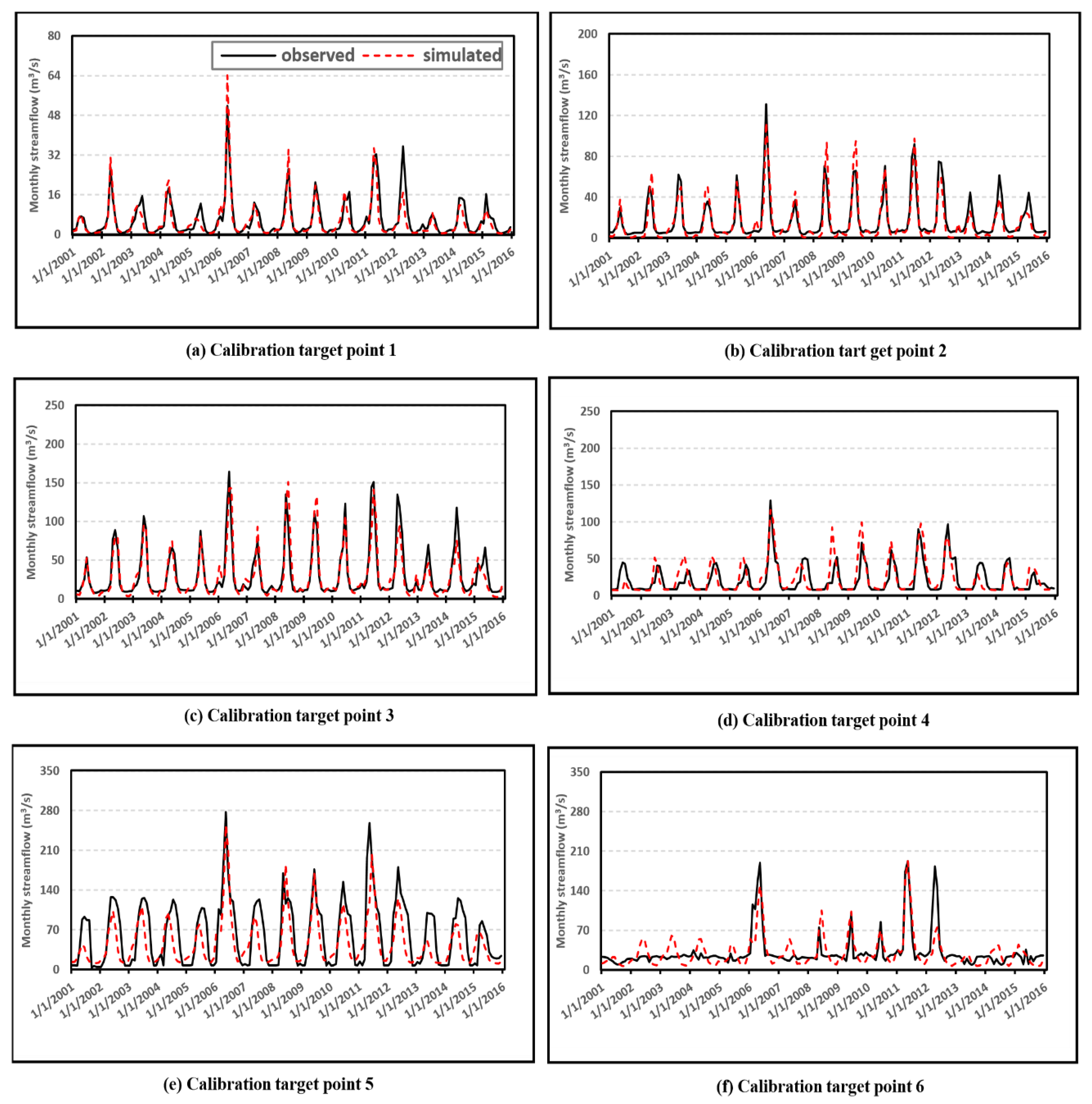
A total of six calibration target points were calibrated from 2001 to 2015 and validated from 1981 to 2000 for streamflow. The initial two years were applied as warm-up periods for calibration (1999 to 2000) and validation (1979 to 1980). Water quality calibration for sediment, TN, and TP were only conducted at the watershed outlet due to the limited observed water quality data. Figure 2 shows hydrographs’ comparison of the monthly observed and simulated streamflow at the calibration target points, and

Table 5. Performance measures of water quality calibration at the watershed outlet.

Performance Statistic	Sediment Load	TN Load	TP Load
R	0.81	0.85	0.85
NSE	0.61	0.51	0.67
RSR	0.63	0.69	0.58
PBIAS (%)	15.32	10.73	8.86

shows the performance measures of water quality calibration at the watershed outlet. Overall, the simulated streamflow closely matched the observed flows. The magnitude of peak flow indicates somewhat different results owing to not only water diversion for irrigation near calibration target point 5 and 6, but also inherent model limitation from reservoir operation rules at the calibration target point 5. Based on the recommend statistics of hydrological model performance at the monthly time step [50], HSPF shows the acceptable performance for calibration and validation at the watershed outlet based on R values for streamflow (above 0.70), sediment load (above 0.8), and nutrient loads (above 0.8) (see Table 5). NSE, RSR, and PBIAS statistics also indicate the fair and good model performance (streamflow, sediment load, and TN load) after calibration.

3.2. Future Climate and Streamflow Variations

Figure 3 shows the projected changes in seasonal precipitation and temperature for the three future time windows (F1: 2021–2045, F2: 2046–2070, F3: 2071–2095) relative to the baseline period (1979–2005). Future precipitation tends to increase substantially in summer by 69.16% and then followed by winter with 34.14% for the F3 period as opposed to the baseline condition. Mean annual precipitation, however, decreases by 2.51% for F1, while it increases by 8.30% and 27.85% for F2 and F3, respectively. Future temperature shows the increasing trend for all three periods as opposed to the baseline. A consistent increase in temperature is observed throughout the future periods under the RCP8.5 scenario. Especially, summer and winter temperatures highly increase over time, while mean annual temperature shows somewhat of a variation (the increasing trend in 3.03 °C, 4.83 °C, and 6.47 °C for F1, F2, and F3, respectively).

Table 6. Future streamflow and water quality variation (Sediment, TN, and TP) associated with the RCP8.5 climate scenario in three different time windows (F1: 2021–2045, F2: 2046–2070, F3: 2071–2095), as opposed to the baseline period (1981–2005).

Component	Baseline	2100 LULC (A2)
		F1	F2	F3	Variation (%)
					F1	F2	F3
Streamflow (m3/s)	31.77	24.10	28.10	32.08	−24.14	−11.19	0.98
Sediment (100 × ton/month)	23.04	25.31	30.02	34.40	9.87	30.30	49.30
TN (ton/month)	94.54	150.61	165.54	174.68	59.31	75.10	84.77
TP (ton/month)	11.25	11.84	12.99	13.63	5.23	15.43	21.16

indicates annual mean variations of streamflow and water quality loads induced by the combined climate variability under RCP8.5 and 2100 LULC associated with the A2 scenario after HSPF calibrations. Annual mean streamflow decreases by 24.14% and 11.19% for F1 and F2, respectively, while it increases by 0.98% for F3 when the combined climate and land use changes are taken into account. The relative change in annual mean sediment load, TN load, and TP load associated with climate variability and land use change show the increasing trend over time for F1, F2, and F3. The period of F3, in particular, shows the most substantial increase in sediment load, TN, and TP by 49.30%, 84.77%, and 21.16%, respectively, as opposed to the baseline. The simulated results under F3, therefore, are used for further analysis to evaluate water management in the study area.

3.3. The Identified Critical Hotspots (CHSs)

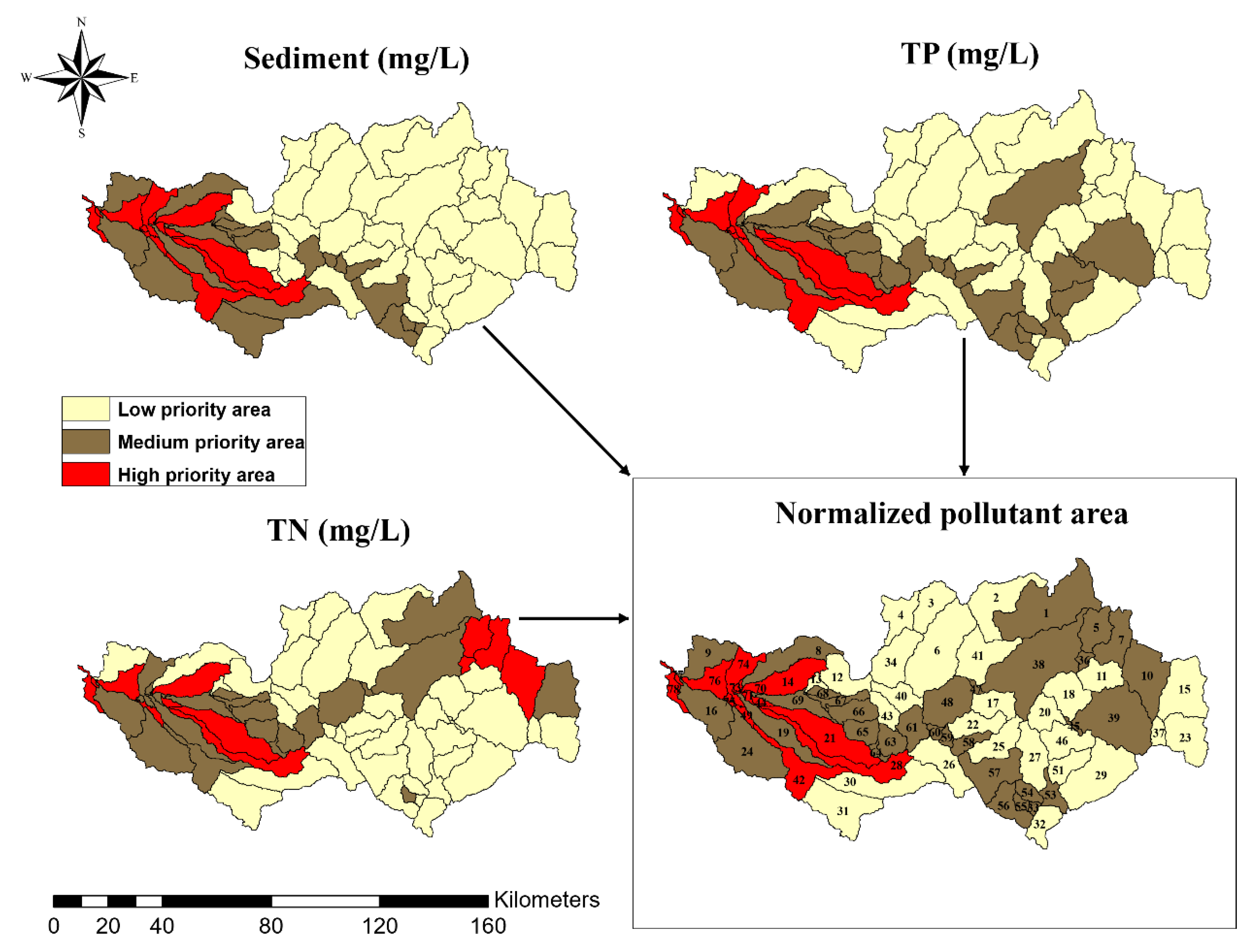
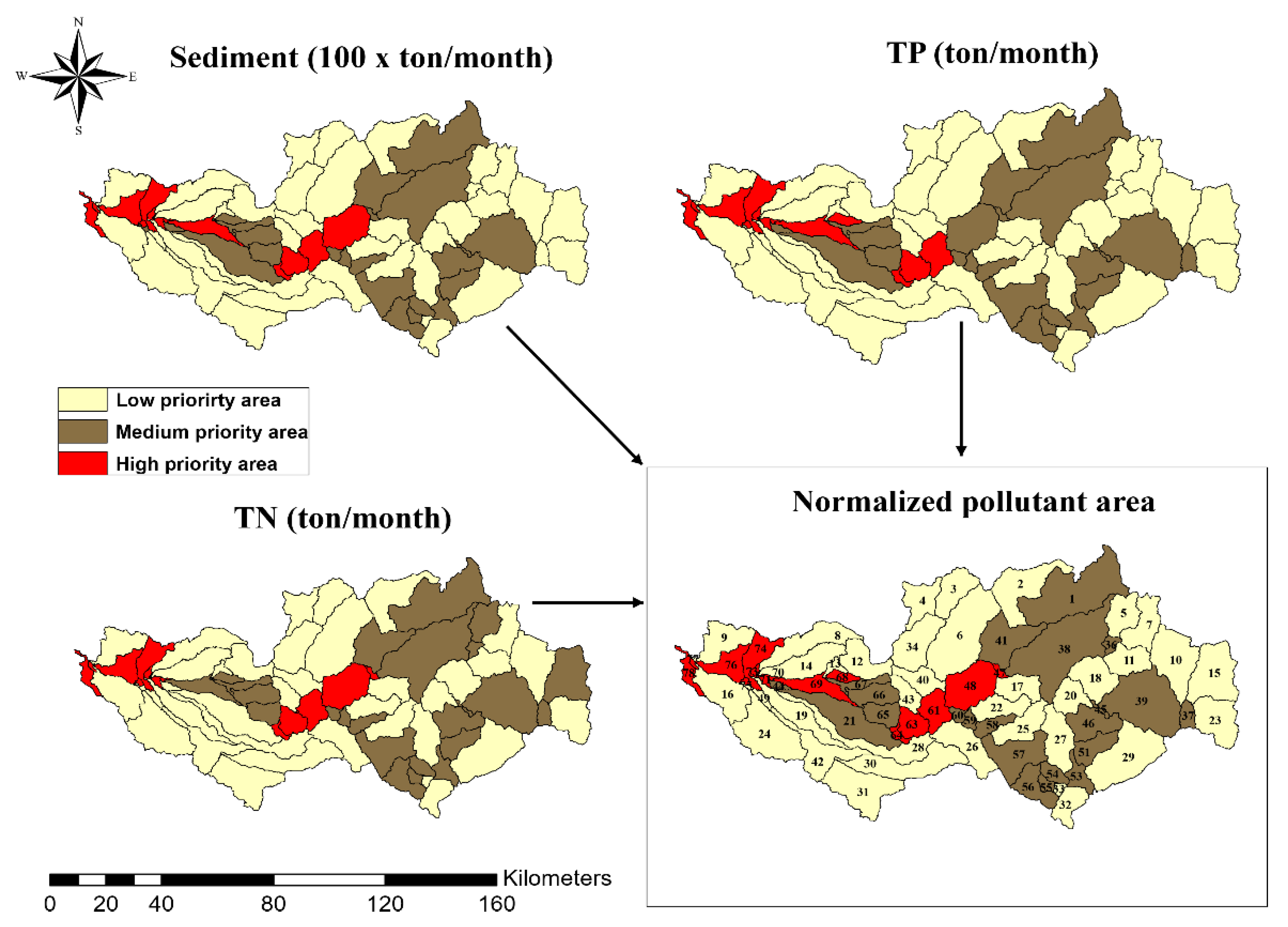
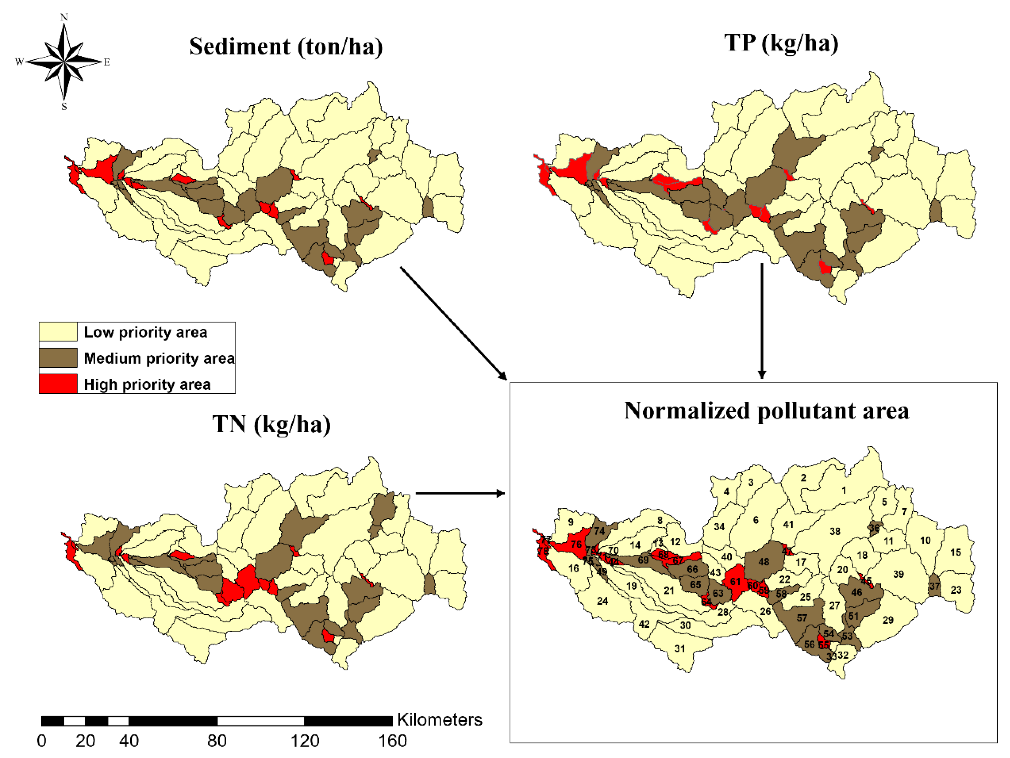
Three indices, including Concentration Impact Index (CII), Load Impact Index (LII), and Load per sub-basin area Index (LPSAI) are used to select critical hotspots (CHSs) in the BRW. As shown in Figure 4, the CII method selects 16 sub-watersheds indicating CHSs (low-, medium-, and high-priority) that are mainly located in the lower Boise watershed below the Lucky Peak dam. It is expected that potential land use change from forestry to marginal/agricultural lands might contribute additional nutrient load (nitrogen) to the Boise River. Similarly, the identified CHSs using the LII method are mostly located in the lower Boise Watershed near the Lucky Peak dam (Figure 5). Perhaps, sediment deposition to the reservoir results in water quality impairment in the middle segment of the Boise River. Unlike CII and LII, LPSAI’s results, however, show very differently in the sense that the identified CHSs are located sparsely across the watershed (see Figure 6). Since the LPSAI method classifies the sub-watersheds with a relatively large amount of pollutants in a small area, significant loads are possibly inherited from upstream to confluences where nutrient converges from small stream segments.

3.4. The Suitable LID/BMP Choice for CHSs

For the identified CHSs above, a decision process to select the best suitable LID/BMP option was carried out based on three different management schemes (EE, EFW, EW) using the AHP structure. The pairwise comparison matrices for CII, LII, and LPSAI are generated as a function of the reduction rate of sediment and nutrient concentration at each sub-watershed level.

Table 7. Pairwise comparison matrix based on sediment reduction at sub-watershed 78 using the CII method.

LID/BMPs	Bioretention	Detention Pond	Filter Strip	Grassed Swale	Wetland
Bioretention	1.00	1.23	2.01	2.28	1.50
Detention pond	0.81	1.00	1.78	2.06	1.27
Filter strip	0.50	0.56	1.00	1.27	0.66
Grassed swale	0.44	0.49	0.79	1.00	0.56
Wetland	0.67	0.79	1.51	1.78	1.00
λmax = 5.004, CI = 0.001, CR = 0.091%.

shows one example of the pairwise comparison matrix for sub-watershed 78 based on sediment reduction using the CII method (not showing all results in this paper). The pairwise comparison matrices of CR (Equation (5)) are calculated 0.091%, 0.001%, 0.01% for sediment, TP, and TN, respectively. Since these CR values are less than 10%, this performance is satisfactory [40]. The weight vector of land feasibility varies depending on slope, drainage area, and land type for an individual sub-watershed.

Table 8. The selected individual LID/BMP at CHSs using spatial targeting methods (CII, LII, and LPSAI) associated with three different weighting schemes (EE, EFW, and EW).

Management Scheme	LID/BMP Types	The Selected CHSs at Sub-Basin Scales
		CII	LII	LPSAI
Equal weight distribution condition (EE)	Grassed swale-LID	13, 21, 42, 44, 76	70, 72, 75, 77	44, 45, 47, 59, 60
	Filter strip-BMP	28, 49, 50, 52, 71, 73, 74, 75, 77, 78	47, 48, 61, 62, 63, 64, 69, 73, 74, 76, 78	55, 61, 62, 64, 68, 71, 72, 73, 76, 77, 78
	Detention pond-LID	72	68, 71	67
Weight on Economic feasibility (EFW)	Filter strip-BMP	44, 45, 47, 55, 59, 60, 61, 62, 64, 67, 68, 71, 72, 73, 78, 77, 78 (all CHSs were selected)
Environmental concern (EW)	Detention pond-LID	14, 21, 42, 44, 72	68, 70, 72, 75, 77	44, 45, 47, 59, 67
	Filter strip-BMP	-	-	55, 60, 61, 62, 64, 68, 71, 72, 73, 76, 77, 78
	Bioretention-LID	28, 49, 50, 52, 71, 73, 74, 75, 76, 77, 78	47, 48, 61, 62, 63, 63, 69, 71, 73, 74, 76, 78	-

shows the selected CHSs associated with their suitable LID/BMP options using three different indices. For example, if a water manager is particularly interested in nutrient concentration (CII) rather than nutrient load (LII or LPSAI), but financial challenge (FC) is inevitable, he or she can select only the filter strip option to be installed at the respective sub-watershed (see Table 8). In contrast, bioretention-LID would be preferable if both nutrient concentration (CII) and nutrient load (LII or LPSAI) are critical, because the environmental concern is evolving in their community. Basically, the water manager can pick and choose the best LID/BMP option to meet their needs.

3.5. Evaluation of LID/BMP Choice

The cost-effectiveness of the management scheme associated with three different indices is summarized in

Table 9. Monthly pollutant load reduction per unit area (kg/ha) and total cost per unit pollutant load reduction ($1000/kg) associated with different management schemes (EE, EFW, and EW).

Management Scheme	Target Method	Load Reduction per Unit Area (kg/ha)				Total Cost per Unit Load Reduction(1000 $/kg)
		Sediment	TN	TP	Mean	Sediment	TN	TP	Mean
Equal weight distribution condition (EE)	CII	7.80	0.10	0.006	2.70	0.43	33.82	552.94	195.73
	LII	8.20	0.06	0.004	2.76	0.42	53.68	916.65	323.58
	LPSAI	12.57	0.07	0.004	4.21	0.27	48.37	813.47	287.37
Weight on Economic feasibility (EFW)	CII	10.66	0.15	0.012	3.61	6.84	496.15	6000.31	2167.77
	LII	10.77	0.09	0.009	3.63	13.31	1537.08	15216.59	5588.99
	LPSAI	11.93	0.09	0.005	4.01	0.44	60.42	1053.50	371.45
Weight on Environmental concern (EW)	CII	7.42	0.13	0.010	2.52	0.95	51.57	740.29	264.27
	LII	8.44	0.07	0.004	2.84	0.50	60.16	1027.46	326.71
	LPSAI	11.16	0.12	0.008	3.76	0.46	44.99	658.76	234.74

to provide useful insights. The pollutant load reduction and efficiency of LID/BMPs vary among their types and location, so the pollutant load reduction per unit area (kg/ha) and total cost per unit pollutant load reduction ($1000/kg) associated with evaluation criteria are great of interest. Overall, filter strip-BMP is the most economical option at the sub-watershed levels compared with other LID/BMP options, while the detention pond-LID and bioretention-LID options are identified as intermediate effectiveness of LID/BMPs due to higher construction cost and pollutant load reduction rate. Thus, when the EE scheme is applied, the results show that LPSAI is the greatest reduction of the average pollutant load by 4.21 kg/ha, while CII is the most cost-effective by 195,728 dollars/kg due to the lower total cost-per-unit pollutant load reduction for TN and TP. Although LPSAI is the greatest reduction of the average pollutant in this particular case, the final decision should be made by the water manager or other decision-maker to select the best LID/BMP out of three options, including Grassed swale-LID, Filter strip-BMP, and Detention pond-LID (see Table 8 and Table 9).

Similarly, when LPSAI is used, the water manager considers that environmental concern is a higher priority so that he/she can select either detention pond-LID or filter strip-BMP. If that is the case, the average pollutant load reduction can be achieved by 3.76 kg/ha, while the cost-effectiveness is reported as $234,736/kg.

4. Summary and Conclusions

The study investigated the potential consequences of climate variability and urbanization associated with land use change on water quality and quantity at the Boise River Watershed over the next few decades. To adapt such consequences, potential water management options, such as LID and BMP, are considered to be implemented in urban (impervious land segment) and rural (pervious land segment) settings. A decision-making process was then proceeded to identify CHSs, to select proper LID/BMP at CHS, and to evaluate the selected LID/BMP options associated with decision factors, including water quality, operational costs, and land feasibility.

A spatial target method using three different indices (CII, LII, and LPSAL) and AHP was then used for CHS identification and LID/BMP selection, respectively. About 8 sub-watersheds out of 78 watersheds are identified as high-priority CHSs using each index, and suitable LID/BMP options are selected and applied accordingly based on different management schemes (economic feasibility, environmental concern). Each LID/BMP option is then evaluated to provide useful insights for water managers to adapt potential consequences in a changing global environment (climate variability and urbanization).

The result shows that only filter strip-BMP is the best option when the economic feasibility is the most critical at the Boise River Watershed, regardless of index values. However, when the environmental concern is the best interest of multiple stakeholders, a water manager may choose the detention pond-LID option as well. It appears that more flexible LID/BMP options are available when all three determining factors (water quality, operational cost, and land feasibility) are treated equally and obviously; a water manager will have more degree of freedom during his decision processes if that is the case. Therefore, these results can strengthen science-based decision-making and provide useful insights to policy-makers in cost-effective water resource management. We anticipate that this informative study can build a case toward developing adaptive water management at the urban–rural interface in a changing global environment. However, in the future, it will be necessary to improve WMT by expanding the number of scenarios through conducting a survey of farmers, water managers, or policy-makers in the watershed to reflect more reliable criteria and their preference for LID/BMPs implementation.

References

1. US.EPA (United State Environmental Protection Agency). National Water Quality Inventory: Report to Congress: 2004 Reporting Cycle; US Environmental Protection Agency, Office of Water: Washington DC, USA, 2009.
2. TNRCC. State of Texas 1998 Clean Water Act Section 303 (d) List and Schedule for Development of Total Maximum Daily Loads; Texas Natural Resource Conservation Commission(TNRCC): Austin, TX, USA, 1998.
3. Dodds, W.K.; Bouska, W.W.; Eitzmann, J.L.; Pilger, T.J.; Pitts, K.L.; Riley, A.J.; Schloesser, J.T.; Thornbrugh, D.J.; Bouska, K. Eutrophication of U.S. Freshwaters: Analysis of Potential Economic Damages. Environ. Sci. Technol. 2009, 43, 12–19. [Google Scholar] [CrossRef] [PubMed] [Green Version]
4. IPCC (Intergovernmental Panel on Climate Change). The Physical Science Basis: Contribution of Working Group I to the Fourth Assessment Report of the Intergovernmental Panel on Climate Change; Cambridge University Press: Cambridge, UK, 2007; pp. 337–383. [Google Scholar]
5. IPCC (Intergovernmental Panel on Climate Change). Climate Change 2013: The Physical Science Basis. Contribution of Working Group I to the Fifth Assessment Report of the Intergovernmental Panel on Climate Change; Cambridge University Press: Cambridge, UK, 2013. [Google Scholar]
6. Giri, S.; Nejadhashemi, A.P.; Woznicki, S.A. Evaluation of targeting methods for implementation of best management practices in the Saginaw River Watershed. J. Environ. Manag. 2012, 103, 24–40. [Google Scholar] [CrossRef] [PubMed]
7. McKinney, D.C.; Cai, X.; Rosegrant, M.W.; Ringler, C.; Scott, C.A. Modeling Water Resources Management at the Basin Level: Review and Future Directions; International Water Management Institute (IWMI): Colombo, Sri Lanka, 1999; Volume ix, 59p. [Google Scholar] [CrossRef]
8. Kaykhosravi, S.; Abogadil, K.; Khan, U.T.; Jadidi, M.A. The Low-Impact Development Demand Index: A New Approach to Identifying Locations for LID. Water 2019, 11, 2341. [Google Scholar] [CrossRef] [Green Version]
9. Kolanuvada, S.R.; Ponpandian, K.L.; Sankar, S. Multi-criteria-based approach for optimal siting of artificial recharge structures through hydrological modeling. Arab. J. Geosci. 2019, 12, 190. [Google Scholar] [CrossRef]
10. Ghebremichael, L.T.; Veith, T.L.; Watzin, M.C. Determination of Critical Source Areas for Phosphorus Loss: Lake Champlain Basin, Vermont. Trans. ASABE 2010, 53, 1595–1604. [Google Scholar] [CrossRef]
11. Panagopoulos, Y.; Makropoulos, C.; Mimikou, M. Decision support for diffuse pollution management. Environ. Model. Softw. 2012, 30, 57–70. [Google Scholar] [CrossRef]
12. Cai, X.; McKinney, D.C.; Lasdon, L. A framework for sustainability analysis in water resources management and application to the Syr Darya Basin. Water Resour. Res. 2002, 38, 21-1–21-14. [Google Scholar] [CrossRef]
13. Li, F.; Liu, Y.; Engel, B.A.; Chen, J.; Sun, H. Green infrastructure practices simulation of the impacts of land use on surface runoff: Case study in Ecorse River watershed, Michigan. J. Environ. Manag. 2019, 233, 603–611. [Google Scholar] [CrossRef]
14. Raei, E.; Alizadeh, M.R.; Nikoo, M.R.; Adamowski, J. Multi-objective decision-making for green infrastructure planning (LID-BMPs) in urban storm water management under uncertainty. J. Hydrol. 2019, 579, 124091. [Google Scholar] [CrossRef]
15. Ryu, J.H.; Palmer, R.N.; Jeong, S.-M.; Lee, J.H.; Kim, Y.-O. Sustainable Water Resources Management in a Conflict Resolution Framework. JAWRA J. Am. Water Resour. Assoc. 2009, 45, 485–499. [Google Scholar] [CrossRef]
16. Roy, B. A multicriteria analysis for trichotomic segmentation problems. Mult. Criteria Anal. Oper. Methods 1981, 8, 245–257. [Google Scholar]
17. Calizaya, A.; Meixner, O.; Bengtsson, L.; Berndtsson, R. Multi-criteria Decision Analysis (MCDA) for Integrated Water Resources Management (IWRM) in the Lake Poopo Basin, Bolivia. Water Resour. Manag. 2010, 24, 2267–2289. [Google Scholar] [CrossRef]
18. Dersseh, M.G.; Kibret, A.A.; Tilahun, S.A.; Worqlul, A.W.; Moges, M.A.; Dagnew, D.; Abebe, W.B.; Melesse, A.M. Potential of Water Hyacinth Infestation on Lake Tana, Ethiopia: A Prediction Using a GIS-Based Multi-Criteria Technique. Water 2019, 11, 1921. [Google Scholar] [CrossRef] [Green Version]
19. Mutikanga, H.E.; Sharma, S.K.; Vairavamoorthy, K. Multi-criteria Decision Analysis: A Strategic Planning Tool for Water Loss Management. Water Resour. Manag. 2011, 25, 3947–3969. [Google Scholar] [CrossRef]
20. Rahman, M.A.; Jaumann, L.; Lerche, N.; Renatus, F.; Buchs, A.K.; Gade, R.; Geldermann, J.; Sauter, M. Selection of the Best Inland Waterway Structure: A Multicriteria Decision Analysis Approach. Water Resour. Manag. 2015, 29, 2733–2749. [Google Scholar] [CrossRef]
21. Ghorbanzadeh, O.; Feizizadeh, B.; Blaschke, T. An interval matrix method used to optimize the decision matrix in AHP technique for land subsidence susceptibility mapping. Environ. Earth Sci. 2018, 77, 584. [Google Scholar] [CrossRef]
22. Bryan, B.A.; Crossman, N.D. Systematic regional planning for multiple objective natural resource management. J. Environ. Manag. 2008, 88, 1175–1189. [Google Scholar] [CrossRef]
23. Santhi, C.; Arnold, J.G.; Williams, J.R.; Dugas, W.A.; Srinivasan, R.; Hauck, L.M. Validation of the Swat Model on A Large Rwer Basin with Point and Nonpoint Sources. JAWRA J. Am. Water Resour. Assoc. 2001, 37, 1169–1188. [Google Scholar] [CrossRef]
24. Cho, J.H.; Sung, K.S.; Ha, S.R. A river water quality management model for optimizing regional wastewater treatment using a genetic algorithm. J. Environ. Manag. 2004, 73, 229–242. [Google Scholar] [CrossRef]
25. Kim, J.; Ryu, J.H. Modeling Hydrological and Environmental Consequences of Climate Change and Urbanization in the Boise River Watershed, Idaho. JAWRA J. Am. Water Resour. Assoc. 2018, 55, 133–153. [Google Scholar] [CrossRef] [Green Version]
26. Chung, E.-S.; Park, K.; Lee, K.S. The relative impacts of climate change and urbanization on the hydrological response of a Korean urban watershed. Hydrol. Process. 2010, 25, 544–560. [Google Scholar] [CrossRef]
27. Jeon, J.-H.; Yoon, C.G.; Donigian, A.S.; Jung, K.-W. Development of the HSPF-Paddy model to estimate watershed pollutant loads in paddy farming regions. Agric. Water Manag. 2007, 90, 75–86. [Google Scholar] [CrossRef]
28. Kim, J.; Ryu, J.H. Quantifying the Performances of the Semi-Distributed Hydrologic Model in Parallel Computing—A Case Study. Water 2019, 11, 823. [Google Scholar] [CrossRef] [Green Version]
29. Mishra, A.; Kar, S.; Raghuwanshi, N.S. Modeling Nonpoint Source Pollutant Losses from a Small Watershed Using HSPF Model. J. Environ. Eng. 2009, 135, 92–100. [Google Scholar] [CrossRef]
30. Yang, Y.; Wang, L. A Review of Modelling Tools for Implementation of the EU Water Framework Directive in Handling Diffuse Water Pollution. Water Resour. Manag. 2009, 24, 1819–1843. [Google Scholar] [CrossRef] [Green Version]
31. Bicknell, B.; Imhoff, J.; Kittle, J., Jr.; Jobes, T.; Donigian, A., Jr. Hydrologic Simulation Program-Fortran (HSPF) User’s Manual for Version 12; US Environmental Protection Agency, National Exposure Research Laboratory: Athens, GA, USA, 2001.
32. Oyj, V. Humidity Conversion Formulas; VAISALA: Helsinki, Finland, 2013. [Google Scholar]
33. Allen, R.G.; Pereira, L.S.; Raes, D.; Smith, M. Crop Evapotranspiration-Guidelines for computing Crop Water Requirements-FAO Irrigation and Drainage Paper 56; FAO—Food and Agriculture Organization of the United Nations: Rome, Italy, 1998. [Google Scholar]
34. USGS (United States Geological Survey). The National Map Download Client. 2015. Available online: https://viewer.nationalmap.gov/basic/ (accessed on 1 January 2018).
35. US.EPA (United State Environmental Protection Agency). Better Assessment Science Integrating Point and Nonpoint Sources (BASINS) Modeling Framework; National Exposure Research Laboratory: Research Triangle Park, NC, USA, 2013. Available online: https://www.epa.gov/ceam/better-assessment-science-integrating-point-and-non-point-sources-basins (accessed on 2 August 2018).
36. Sohl, T.L.; Sayler, K.L.; Bouchard, M.A.; Reker, R.R.; Friesz, A.M.; Bennett, S.L.; Sleeter, B.M.; Sleeter, R.R.; Wilson, T.S.; Soulard, C.; et al. Spatially explicit modeling of 1992–2100 land cover and forest stand age for the conterminous United States. Ecol. Appl. 2014, 24, 1015–1036. [Google Scholar] [CrossRef]
37. Schreüder, W.A. Running BeoPEST. In Proceedings of the 1st PEST Conference, Potomac, MD, USA, 2–4 November 2009. [Google Scholar]
38. Doherty, J.; Skahill, B.E. An advanced regularization methodology for use in watershed model calibration. J. Hydrol. 2006, 327, 564–577. [Google Scholar] [CrossRef]
39. Tuppad, P.; Srinivasan, R. Bosque River Environmental Infrastructure Improvement Plan: Phase II BMP Modeling Report; Texas AgriLife Research; Texas A&M University: College Station, TX, USA, 2008. [Google Scholar]
40. Saaty, T.L. The Analytic Hierarchy Processes; McGraw-Hill: New York, NY, USA, 1980. [Google Scholar]
41. US.EPA (United State Environmental Protection Agency). HSPF Version 12.4. User’s Manual; National Exposure Research Laboratory: Research Triangle Park, NC, USA, 2014.
42. Banai, R. Fuzziness in Geographical Information Systems: Contributions from the analytic hierarchy process†. Int. J. Geogr. Inf. Syst. 1993, 7, 315–329. [Google Scholar] [CrossRef]
43. Zhu, X.; Dale, A. JavaAHP: A web-based decision analysis tool for natural resource and environmental management. Environ. Model. Softw. 2001, 16, 251–262. [Google Scholar] [CrossRef]
44. Nagaraju, D.; Nassery, H.; Adinehvandi, R. Determine suitable sites for artificial recharge using hierarchical analysis process (AHP), remote sensing and geographical information system. Int. J. Earth Sci. Eng. 2012, 5, 1328–1335. [Google Scholar]
45. Brown, W.; Schueler, T. The Economics of Stormwater BMPs in the Mid-Atlantic Region; Center for Watershed Protection: Silver Spring, MD, USA, 1997. [Google Scholar]
46. County, F. National Pollutant Discharge Elimination System; Anne Arundel County Department of Public Works: Annapolis, MD, USA, 2014. [Google Scholar]
47. Dhalla, S.; Zimmer, C. Low Impact Development Stormwater Management Planning and Design Guide, Version 1.0; Toronto and Region Conservation for the living city: Toronto, ON, Canada, 2010. [Google Scholar]
48. NCDENR (North Carolina Department of Environment and Natural Resources). Stormwater BMP Costs; NCDENR: Raleigh, NC, USA, 2007.
49. US.EPA (United State Environmental Protection Agency). Preliminary Data Summary of Urban Storm Water Best Management Practices; United States Environmental Protection Agency, Office of Water: Columbus, OH, USA, 1999. Available online: http://www.epa.gov/waterscience/guide/stormwater/#nsbd (accessed on 1 January 2019).
50. Moriasi, D.N.; Arnold, J.G.; Van Liew, M.W.; Bingner, R.L.; Harmel, R.D.; Veith, T.L. Model Evaluation Guidelines for Systematic Quantification of Accuracy in Watershed Simulations. Trans. ASABE 2007, 50, 885–900. [Google Scholar] [CrossRef]
51. Sadeghi, S.H.; Jalili, K.; Nikkami, D. Land use optimization in watershed scale. Land Use Policy 2009, 26, 186–193. [Google Scholar] [CrossRef]
52. Nash, J.E.; Sutcliffe, J.V. River Flow forecasting through conceptual models-Part I: A discussion of principles. J. Hydrol. 1970, 10, 282–290. [Google Scholar] [CrossRef]
53. LeGates, D.R.; McCabe, G. Evaluating the use of “goodness-of-fit” Measures in hydrologic and hydroclimatic model validation. Water Resour. Res. 1999, 35, 233–241. [Google Scholar] [CrossRef]
54. Gupta, H.V.; Sorooshian, S.; Yapo, P.O. Status of Automatic Calibration for Hydrologic Models: Comparison with Multilevel Expert Calibration. J. Hydrol. Eng. 1999, 4, 135–143. [Google Scholar] [CrossRef]
Figure 1. The map of the Boise River Watershed (BRW).
Water 12 02436 g001
Figure 2. Comparisons of the simulated and observed streamflow at the calibration target points 1–6, (af), respectively.
Water 12 02436 g002
Figure 3. Future precipitation (a) and temperature (b) variations associated with RCP8.5 climate scenarios in three different time windows (F1: 2021–2045, F2: 2046–2070, F3: 2071–2095), as opposed to the baseline period (1981–2005).
Water 12 02436 g003
Figure 4. The identified critical hot spots (CHSs) using the CII method.
Water 12 02436 g004
Figure 5. The identified critical hot spots (CHSs) using the LII method.
Water 12 02436 g005
Figure 6. The identified critical hot spots (CHSs) using the LPSAI method.
Water 12 02436 g006