Validation of Machine Learning Models for Structural Dam Behaviour Interpretation and Prediction

Abstract

The main aim of structural safety control is the multiple assessments of the expected dam behaviour based on models and the measurements and parameters that characterise the dam’s response and condition. In recent years, there is an increase in the use of data-based models for the analysis and interpretation of the structural behaviour of dams. Multiple Linear Regression is the conventional, widely used approach in dam engineering, although interesting results have been published based on machine learning algorithms such as artificial neural networks, support vector machines, random forest, and boosted regression trees. However, these models need to be carefully developed and properly assessed before their application in practice. This is even more relevant when an increase in users of machine learning models is expected. For this reason, this paper presents extensive work regarding the verification and validation of data-based models for the analysis and interpretation of observed dam’s behaviour. This is presented by means of the development of several machine learning models to interpret horizontal displacements in an arch dam in operation. Several validation techniques are applied, including historical data validation, sensitivity analysis, and predictive validation. The results are discussed and conclusions are drawn regarding the practical application of data-based models.

1. Introduction

Dam safety is a continuous requirement due to the potential risk of environmental, social, and economic disasters. In ICOLD’s bulletin number 138 [1] the assurance of the safety of a dam or any other retaining structure is considered to require “a series of concomitant, well-directed, and reasonably organised activities. The activities must: (i) be complementary in a chain of successive actions leading to an assurance of safety, (ii) contain redundancies to a certain extent so as to provide guarantees that go beyond operational risks” [1]. Continuous dam safety control must be done at various levels. It must include an individual assessment (dam body, its foundation, appurtenant works, adjacent slopes, and downstream zones) and, as a whole, in the various areas of dam safety: environmental, structural, and hydraulic/operational [2].

Structural safety can be understood as the dam’s capacity to satisfy the structural design requirements, avoiding accidents and incidents during the service life. Structural safety includes all activities, decisions, and interventions necessary to ensure the adequate structural performance of the dam. The activities performed for the structural safety control of large dams are usually aided by simulation models. According to Lombardi [3]: “the difference between the predicted value and the actual reading is indeed the true criteria to judge the behaviour of the dam”. Such predictions can be based on deterministic models, such as finite element models or data-based models. Most large dams have an essential database of monitoring measurements, recorded along years, both from the environmental variables (related to the main loads) and the dam response. This, together with the developments in Machine Learning (ML) techniques, has led to a significant increase in the use of ML models to support the analysis and interpretation of the observed structural behaviour. The ML algorithms applied [4] include multiple linear regressions [3,5,6], artificial neural networks [7,8,9,10,11,12,13,14,15,16], support vector machines [17,18], random forest [19] and boosted regression trees [20]. A comparison of their performance can be found in [21].

Regression models are the most known and used data-based models for engineers responsible for dam safety activities. They have been validated and tested over years of use, and their capabilities and limitations are well known [21]. In recent years, new data-based models based on ML methods have been adopted as a guaranty in redundancy to the traditional adopted models to describe the observed behaviour or, in some cases, to study a particular aspect of the dam behaviour. However, the growing use of ML models is mainly restricted to scientific publications and academic examples, without a broad and deep discussion about model validation and verification issues. These research and technical gaps are partly because of the lack of agreement regarding how to reliably evaluating the validity of these models and their scope of application. Open issues for their practical implementation include:

• The adequate selection of input variables.
• The possibilities and limitations of their interpretation for identifying the effects of the external variables.
• The required size of the available monitoring data for model fitting.
• The methods for handling missing values.
• The selection of training and predicted sets.
• The procedure for reliably evaluating model accuracy and defining warning thresholds from model predictions.

In other fields with extended background on the application of data-based models, a further effort was put into developing procedures and concepts for model validation. This is the case of electrical engineering, where Sargent [22] proposed an overall framework for verifying and validating simulation models in any area of expertise.

The problem is more relevant in social sciences, where the decisions of the modeller have a substantial effect on the results because of the higher indetermination in the definition of the prediction task (e.g., [23]). Likewise, when complex databases are used, different decisions may lead to opposite conclusions [24].

The main contribution of this work is the presentation of a methodology for the validation and verification of ML models to the analysis and interpretation of the structural behaviour observed in dams. In this work, Sargent’s framework is adapted to dam safety for the validation and verification of data-based models for predicting dam behaviour. The proposed approach is applied to the case study of an arch dam located in Portugal. Models based on neural networks (NN), support vector machines (SVM), random forests (RF), and boosted regression trees (BRT) are fitted for predicting the radial displacement of the highest cantilever. The results are discussed, and conclusions are drawn regarding their application in practice.

The article is organised as follows: Section 2 includes a state of art review regarding the adoption and use of ML models to analyse and interpret the observed structural dam behaviour. The proposed methodology for model validation and verification is presented in Section 3. The case study is described in Section 4. The results of the application of the proposed methods for validation and verification are presented and discussed in Section 5. Finally, conclusions are included in Section 6.

2. State of Art: Machine Learning Models for Dam Behaviour Interpretation and Prediction

2.1. Overview about Machine Learning

Machine Learning is usually described as the study of “computer algorithms that improve automatically through experience” [25]. There are two main ML approaches used in different problems: supervised and unsupervised learning, Figure 1. In unsupervised learning, only the input data is available. The objective is to define groups or classes of similar samples, then assigning some class to new inputs. In supervised learning, both the input variables and the true output of the system are available during the training stage. The algorithm learns the association between inputs and response so that predictions can be obtained when new inputs are provided to the model. Supervised learning is the approach used in dam safety, using measured data from the past behaviour of the dam for model fitting.

Supervised models can in turn be classified into regression, if the output variable is numerical, and classification, in case it is categorical. Although some applications of classification in dam safety can be found in the literature [26,27], the vast majority of examples of ML models in this field are based on regression.

As a result, only supervised regression models are considered in this work. Several mathematical algorithms can be adopted, depending on the goal and the data available, Figure 2. A description of the main algorithms used in the context of the interpretation of the behaviour of dams can be found in [4,21]. As mentioned above, NNs, RF, SVM and BRT are considered in this application. These algorithms are succinctly described herein, together with the conventional multiple linear regression model, which is taken as reference.

The regression problem in dam safety can be formulated as follows: suppose that a dataset with p independent variables and n observations, $\left(X_1,\dots ,X_p,Y\right)$ is available, where Y represents the observed structural response, and X are the functions of water height above the dam base, temperature and time. The goal of a regression model is computing an estimate of the response variable as a function of the inputs (Equation (1)):

$$Y = f\left(X_j\right) + ϵ, j = 1\dots p$$

(1)

where $ϵ$ is the model error.

The overall process for building and applying data-based predictive models is summarised in Figure 3. The monitoring data available is split into two separate datasets. The former is used to calibrate the model parameters (e.g., number of neurons in a NN model), while the latter is fed into the calibrated model for verifying prediction accuracy. Some authors use all available data for training, which may be acceptable if regression models are used. However, leaving an independent data set for model evaluation is essential for most ML models to avoid overfitting.

2.2. Formulation by Separation of the Reversible and Irreversible Effects: The HST and HTT Approaches

In the operation phase of the dam’s life, the thermal effect is directly related to the air and water temperature variations. There are two main approaches for choosing the parameters that represent the thermal effect in data-based models [6]: the $HST$ (hydrostatic, seasonal, time) approach and the $HTT$ (hydrostatic, temperature, time) approach. In the $HST$ approach, the portion of the structural response due to the thermal effects is usually considered as the sum of sinusoidal functions with an annual period, similar to air and water temperatures variations. As a result, the thermal effects are smoothed. In the $HTT$ approach, the thermal effects are associated to temperatures measured on the dam body, therefore, the actual evolution of thermal loads is considered. Although some authors have presented the benefits of using measured temperatures of the concrete dam body with, or instead of, sinusoidal functions [5], $HTT$ models are not often used in day-to-day analysis analysis because of the difficulty in the selection of the variables to represent the thermal effect, especially when there is a large number of input variables. In this work, the $HST$ was the approach adopted to obtain the main results. More details regarding the input variables usually adopted in this type of model can be found in [5,6,7,21,28].

The data-based models used for the prediction of the structural response of concrete dams are based on the following simplifying assumptions:

(i)

The analysed effects refer to a period in the life of a dam for which there are no relevant structural changes.

(ii)

The effects of the normal structural behaviour for normal operating conditions can be represented by two parts: a part of elastic nature (reversible and instantaneous, resulting from the variations of the hydrostatic pressure and the temperature) and another part of the inelastic nature (irreversible) such as a time function.

(iii)

The effects of the hydrostatic pressure, temperature, and time changes can be evaluated separately.

2.3. Machine Learning Models Used for the Dam Behaviour Interpretation and Prediction

Multiple Linear Regression (MLR) models are widely used by dam engineers. The form of Equation (1) for a MLR model relating the independent variables to the dependent variable can be written as (Equation (2)):

$$Y = {\beta }_0 + {\beta }_1{X}_1 + {\beta }_2{X}_2 +\dots + {\beta }_j{X}_j +\dots + {\beta }_p{X}_p + ϵ$$

(2)

where $ϵ$ stands for the random error. The model can be represented by a system of n equations that can be expressed in a matrix notation as $\mathit{Y} \mathbf{=} \mathit{X}\mathit{\beta } \mathbf{+} \mathit{ϵ}$ where Y is a ($n \times 1$) vector of the dependent variable or response, X is a ($n \times \left(p+1\right)$) matrix of the levels of the p independent variables, $\mathit{\beta }$ is a ($\left(p + 1\right) \times 1$) vector of the regression coefficients, and $\mathit{ϵ}$ is a ($n \times 1$) vector of random errors.

The model assumes that the expected value of the random error is zero, i.e., $E\left(\mathit{ϵ}\right) = 0$; the variance $V\left(\mathit{ϵ}\right) = {\sigma }^2$ and the errors are uncorrelated [29,30,31]. In matrix notation, the least squares estimator of $\mathit{\beta }$ is $\widehat{\mathit{\beta }} = {\left({\mathit{X}}^{\mathit{T}}\mathit{X}\right)}^{-1}{\mathit{X}}^T\mathit{Y}$ while the fitted model is $\widehat{\mathit{Y}} = \mathit{X}\widehat{\mathit{\beta }}$ and the vector of the residuals is denoted by $\widehat{\mathit{ϵ}} = \mathit{Y} - \widehat{\mathit{Y}}$.

The general expression of the regression problem shown in Equation (1) applies to ML regression models. However, the final mathematical expression is in general more complex than that of the MLR, and, therefore, more difficult to analyse.

Neural networks can be considered as an extension of MLR models by adding a non-linear transformation of the inputs [32]. The output of the model is computed as presented in Equation (3):

$$y_{NN} = \sum _{l=1}^L{w}^l·g\left(X_t\right) + b$$

(3)

where L is the total number of neurons in the hidden layer, $w^l$ are the weights, $X_t$ is a linear transformation of the inputs $X_j$, and $g\left(X_t\right)$ is a non-linear transformation. In this work, a sigmoid function is used in the hidden layer, different for each neuron l, which is computed as presented in Equation (4):

$$g\left(X_t\right) = \frac{1}{1+e^{X_t}}$$

(4)

Many variations of the original NN model have been proposed and used in different fields: from the addition of several intermediate layers until the introduction of complex algorithms to account for certain aspects of the model [33,34]. NN can be considered the most popular ML algorithm in dam engineering [7,10,17].

In general, NN are prone to overfitting, i.e., their high flexibility allows for increasing the prediction accuracy for the training data (in theory, perfect accuracy could be achieved [35]). This issue can be alleviated using cross-validation or similar resampling techniques.

However, this does not imply that such model will be as accurate for an independent data set. Therefore, the training process needs to be followed with care. An independent data set needs to be considered to evaluate the model, for which prediction error should be similar to that in the training set.

Support vector machines resemble NNs in some aspects, such as the inclusion of non-linear transformations of the inputs. In this case, the inputs are transformed, then linear regression is performed on the modified variables. Overfitting is also an issue for SVM models, and the training parameters strongly influence the results. Consequently, SVM models must be fitted with care: wide ranges of parameter values need to be considered, and cross-validation or similar approaches must be followed to obtain reliable estimates on the prediction accuracy. SVM have been used in some publications related to dam safety, but the effect of the model parameters was not examined in depth [4,11,17,21].

Other ML algorithms recently applied to the prediction of dam behaviour belong to the family of tree-based models: random forests (RF) and boosted regression trees (BRT). In both cases, the model outcome is computed from a typically large amount of simple models, in this case, regression trees.

Regression trees are often used in classification problems because of their ease of interpretation: usual rules can be represented by these models in the form of criteria for dividing the original dataset into a series of groups with common features. However, such approach can also be applied for regression, i.e., for predicting numerical variables, by computing the average of the output variable for all elements in each of the resulting groups. This approach keeps the interpretability, but prediction accuracy is lower than for other algorithms. In addition, the resulting model is strongly dependent on the training set, i.e., the addition of a few samples may result in highly different rules and predictions. To overcome the limitations of regression trees, RF were proposed by Breiman [36], in which a significant amount of simple regression trees is created, and the result is computed as the average of their predictions. Additional ingredients of the RF algorithm include:

• Each tree is created from a bootstrapped sample of the training set, in which some the samples are included, some are excluded, and others are duplicated.
• Only a random subsample of the inputs is taken for creating each split of each tree.

RF models are easy to implement and robust in complex settings [36], particularly when the $\frac{p}{n}$ ratio is high [37].

BRTs are also based on trees, with some differences:

• The tree models in the ensemble are simple, i.e., with just a few branches.
• Each tree is fitted on a random subset of the original training set.
• The residual of the previous ensemble is considered as the objective function for fitting each tree. As a result, the model prediction is computed as the sum of outputs from all trees (instead of the average, as for RF).

BRTs share some of the advantages of RFs regarding their robustness (low dependence on the training parameters) and a lower tendency to overfitting [20].

An in-depth description of the mathematical foundation of these algorithms is out of the scope of this article. They can be found in many publications with different viewpoints, from theory to practice, a selection of which is included in

Table 1. Reference publications on the ML algorithms considered.

	Relevant Publications
Algorithm	Theory and Fundamentals	Practical Implementation
Neural networks	[35]	[7,8]
Support Vector Machines	[38,39]	[18,40,41]
Random Forests	[36]	[19,42]
Boosted Regression Trees	[43,44]	[20,45]

.

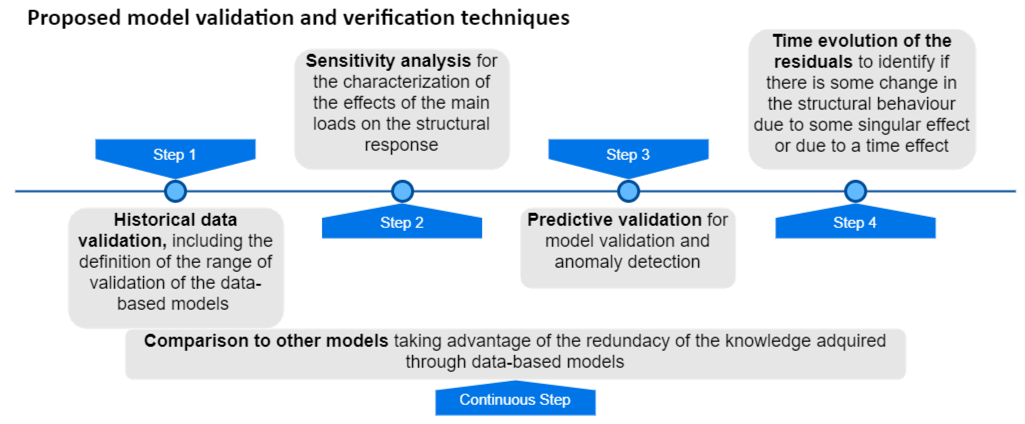
3. Methodology Proposed for Model Validation and Verification

The main concepts coined for general verification and validation of simulation models can be summarised, based on Sargent’s framework [22], as follows:

• Model verification is “ensuring that the computer program of the computerized model and its implementation are correct”.
• Model validation is a “substantiation that a computerized model within its domain of applicability possesses a satisfactory range of accuracy consistent with the intended application of the model”.
• Model accreditation is determining if a model satisfies specified model accreditation criteria according to a specified process.
• Model credibility is the concern with developing in (potential) users the confidence they require to use a model and in the information derived from that model.

A model may be valid for one set of experimental conditions and invalid for another. Performing model verification and validation is usually part of the (entire) model development process. The graphical paradigm developed by Sargent [22] was adapted for dam engineering (Figure 4).

These definitions presented by Sargent [22] were updated for the case of data-based models in the field of dam safety and dam engineering. Thus, specialists in dam safety activities can consider the verification and validation of ML models for the interpretation of structural dam’s behaviour that:

(i)

The problem entity is the system (real) composed of the reservoir, the dam and its foundation.

(ii)

The conceptual model is the mathematical/logical/verbal representation of the problem entity developed for a particular study, usually the analysis and interpretation of the observed structural dam’s behaviour (based on recorded data).

(iii)

The computerized model is the conceptual model implemented on a computer. In this case, machine learning was adopted for the development of the model simulation. A critical aspect of this topic is that the person who develops the ML model (as a programmer or as a software user) must have a strong knowledge of how machine learning techniques work and be familiarized with the programming language or with the software in use.

(iv)

The conceptual model validation is defined as determining that the theories and assumptions underlying the conceptual model are correct and that the model representation of the problem entity is “reasonable” for the intended purpose of the model. For example, dam engineers usually perform this validation through the following questions: Is the horizontal displacement of the dam body increasing with the increase of hydrostatic water effect? Is the displacement downstream or upstream? Is the range of displacements higher near the crest? Is the structural response due to the air temperature variations similar to a sinusoidal shape with an annual period? Can the effects of the hydrostatic pressure, temperature, and time changes be evaluated separately?

(v)

Computerized model verification is defined as assuring that the computer programming and implementation of the conceptual model are correct. In the case of data-based models used in dam engineering, this is performed through the knowledge of the functioning, the field of application and the range of validity of the machine learning methods. The computerized model is developed and tested to verify if the conceptual model is well simulated using a “training set” of data from the reservoir-dam-foundation system (problem entity). For the computerized model verification, two types of verifications can be performed: (i) the first regarding the verification of the programming code (if a home-made software is used) or regarding parameters and to the learning method adopted in each case, and (ii) the second regarding the verification of the conceptual model must be supported by a specialist with a strong knowledge about the dam’s behaviour.

(vi)

Operational validation is defined as determining that the model output behaviour has sufficient accuracy for the intended purpose over the domain of the intended applicability. This is usually achieved through the knowledge of the performance indicators of the data-based models developed. In some cases, a new set of data from the reservoir-dam-foundation system is used to validate the model.

(vii)

Data validity is defined as ensuring that the data necessary for model building, evaluation and testing, and conducting the model experiments to solve the problem are adequate and correct. This is an important task usually performed through the quality control of monitoring data—e.g., repeatability and reproducibility studies [46], comparison between manual and automated measurements [47], the metrological verification of the measuring devices [48], training of the operators, and through the quantification of the measurement uncertainties in dam monitoring systems.

Verification and validation must be performed again when any change is made to the model. For problem entity, some changes can result from some incident, change in the properties of the dam body (e.g., due to changes in concrete proprieties due to alkalis-silica reactions) or even improvement works performed in the structure or surrounding, e.g., due to tunnel excavations near the dam body for the construction of power boosts. In typical situations, these models are used to characterize the pattern of the structural dam behaviour in normal conditions of exploitation and then identify possible changes in the structural condition of the dam.

In addition to the work used as the primary reference, several works [49,50,51,52,53,54] present several validation techniques in different areas of expertise. Some of them have been used in dam engineering for the validation of traditional models.

Based on the referred before, the authors propose the adoption of the following techniques for the verification and validation of ML models for dam behaviour interpretation: historical data validation, parameter variability-sensitivity analysis, predictive validation, comparison to other models, and analysis of the time evolution of the residuals, as presented in Figure 5 and succinctly described in

Table 2. Description of the proposed techniques for model validation and verification of ML models for dam behaviour interpretation, adapted from [22].

Validation Technique	Description
Historical data validation	Part of the data is used to build the model, and the remaining data are used to determine (test) whether the model reproduces the behaviour of the system.
Sensitivity analysis	The values of the input variables are changed and the effect on the model output is analyzed, which should resemble the observed behaviour of the real system. This technique can be used qualitatively—directions only of outputs—and quantitatively—both directions and (precise) magnitudes of outputs.
Predictive validation	The model is used to generate predictions of the behaviour of the system, which are later compared to the observed response to identify anomalies and draw conclusions regarding the safety state of the dam. The data may come from an operational system or be obtained by conducting experiments on the system, e.g., field tests.
Comparison to other models	This action is transversal and is performed for all three previous processes, i.e., results of different models in terms of historical data validation, sensitivity analysis, and predictive validation are compared and discussed.
Time evolution of the residuals	This action allows to easily identify if there are singularities on the observed behaviour or sometrend (such as a change of the observed pattern) over time.

.

In dam engineering, the HST approach is consensually accepted, as referred before. This approach assumes that the effects of the main loads (water level and temperature variations) on the structural response can be considered independently (known as separation effects). This can be checked by applying a sensitivity analysis as proposed in this work. Indirectly, the potential risk of dams (low probability of accident but with very high consequences) is an aspect that justifies the need for robust model validation and verification process.

The mathematical calculation and the graphic representation presented in the following sections were supported by the R project software and several packages [55,56,57,58,59,60,61,62].

4. Case Study

4.1. The Salamonde Dam

Salamonde dam (Figure 6) is located in the Cávado River, which flows through north-western Portugal, being part of the hydro-electrical system of Cávado-Rabagão-Homem owned and operated by EDP [63]. The Salamonde dam consists of a double curvature arch. The construction completion date was 1953. The maximum dam height is 75 m, and the total crest length is 284 m. The maximum reservoir water level is 280.0 m, with a total storage capacity of 65 hm${}^3$. Following the best technical practices, the monitoring system of the Salamonde dam aims at the evaluation of the loads, the characterization of the rheological, thermal and hydraulic properties of the materials, and the evaluation of the structural response.

The monitoring system of the Salamonde dam consists of several devices, which measure physical quantities such as concrete and air temperatures, reservoir water level, seepage and leakage, displacements in the dam and on its foundation, joint movements, and pressures, among others. The deformation of the dam body is controlled with five inverted pendulums (FP1 to FP5).

In this case study, the measurements of the (absolute) horizontal displacements (radial direction) measured at the highest base (at 277.07 m) of the combined FP3 and FP5 pendulums is analysed (FP3/5–277.07 m). The location of the FP3/5–277.07 m base is shown in Figure 6.

4.2. The Analysed Data

The data analysed corresponds to a period between January 2000 and December 2019, resulting in more than 934 observations per variable. The data between January 2000 and December 2014 was used for training the ML models. The dam behaviour and its structural condition during the period of the training set, are considered adequate by the dam engineering specialists. So, the main purpose is to obtain ML models able to represent the behaviour pattern observed in the training set with a good generalization capability. Once the ML models are generated, the purpose is to use them in the day-to-day dam monitoring and safety activities. Thus, the data from the time period between January 2015 and December 2019 was adopted as a predicted set. The time evolution of the reservoir water level and radial displacements in the referred FP3/5–277.07 m base are presented in Figure 7. The statistical characterization of the radial displacement and of the water height variations is presented

Table 3. Statistical parameters for the radial displacement measured in the FP3/5–277.07 m and for the reservoir water level.

		Radial displ. (mm)		Water Height (m)
		Training Set	Predicted Set	Training Set	Predicted Set
Mean	(mm)	14.49	9.90	66.16	69.09
Max	(mm)	39.9	26.9	74.1	73.46
Min	(mm)	−4.1	−3.5	45.8	62.64
$\sigma$	(mm)	10.58	7.69	6.60	2.60

.

The structural response of the displacement at any point of the dam is strongly related to the corresponding variation in the water level in the reservoir. The observations presented in Figure 7 were used for the computation of the models presented in this work. Signs (+) indicate displacements towards upstream and signs (−) towards downstream.

A characterization and knowledge of the main data prior to any deep analysis are essential to avoid misinterpretation of the dam behaviour. One part of this task is usually performed through expedite data visualization, as presented in Figure 7. Figure 8, Figure 9, Figure 10 and Figure 11 can also support this first analysis in order to identify the domain of the training set, in terms of (i) the water level (Figure 8 and Figure 9) and also the thermal (indirectly to the range of data in a month) loads and, (ii) in terms of the displacements observed (Figure 10 and Figure 11).

4.3. The ML Models Developed

Once a basic knowledge about the main loads’ variations and radial displacement is achieved, the ML models were developed following the HST approach. The ML methods used were: the Multiple Linear Regression (MLR), Support Vector Machine (SVM), Multilayer Perceptron Neural Network (NN), Random Forest (RF) and Boosted Regression Trees (BRT).

Although different ML models were considered in this work, the article focuses on the methods and criteria for model validation and verification rather than on the implementation of these models or their capabilities and limitations. This implies that the models showed are not optimal, but they present an adequate generalization capacity. In general, default training parameters were considered and a reduced amount of input variables was included, being the same terms used for all models.

The MLR model was used for comparison since it is widely used and well known in the dam engineering community. In addition, the radial displacement of an arch dam was chosen, for which the HST approach is appropriate.

In this case study, the MLR model with the best performance for the radial displacement of the FP3/5–277.07 m, $y_{MLR}$ was obtained as the sum of the hydrostatic pressure term ${\beta }_4 \times h^4$ (where h is the reservoir water level height and can vary between 0 and 75 m) and the temperature terms ${\beta }_5 \times \sin \left(d\right) + {\beta }_6 \times \cos \left(d\right)$ to represent the effect of the annual thermal variation of the temperature, where $d = \frac{2\pi j}{365}$ and j is the number of days between the beginning of the year and the date of the observation. No relevant variation was recorded on the past behaviour of Salamonde Dam. This was verified in preliminary fits of the MLR model, including time-dependent terms. The results (not shown) confirm the negligible effect of time. Therefore, no time effect was considered in any ML model.

The input variables ($h^4$, $\sin \left(d\right)$ and $\cos \left(d\right)$) were used in the same form in all the ML models. They were previously transformed in order to vary between zero and one. The regression coefficients of the MLR models obtained are ${\beta }_4$ = −26.445, ${\beta }_5$ = −12.378 and ${\beta }_6$ = −12.624, with ${\beta }_0$ = 42.125; being the MLR model represented through the Equation (5).

$$y_{MLR} = -26.445h^4 - 12.378\sin \left(d\right) - 12.624\cos \left(d\right) + 42.125$$

(5)

The residuals were obtained through the difference between the observed horizontal displacement and the corresponding predicted value. These values contain all information that the model cannot explain.

Regarding the development of the remaining ML models:

• SVR model: a Gaussian RBF kernel with an $ϵ$-insensitive loss function was adopted and several values of $ϵ$ (0.05, 0.1, 0.5), C (1, 10, 20) and $\gamma$ (0.1, 0.2, 0.3, 0.4) were tested on 2/3 of the training data, and their accuracy evaluated on the remaining 1/3. The best combination of parameters were $ϵ$ = 0.1, C = 10 and $\gamma$ = 0.3.
• NN model: Every neuron in the network is fully connected with each neuron of the next layer. A logistic transfer function was chosen as the activation function for the hidden layer and the linear function for the output layer. Parameter calibration was used for the NN model to select the number of neurons in the hidden layers: models with 3, 4 and 5 neurons were tested. To find out the optimum result, 15 initializations of random weights and a maximum of 1500 iterations were performed for each NN architecture. A cross-validation technique was adopted to select the best NN: 65% of the training set was used for training, 20% of the training set was used to choose the NN with better performance and 15% of the training set was used to check the performance of the NN model.
• RF model: Default parameters were used for the RF model, i.e., 500 trees and one input variable randomly taken for each split.
• BRT model: Default parameters of the gbm package [62] were applied, with 300 trees in the final model.

Higher prediction accuracy may be obtained for the case study after a throughout selection of variables and model calibration, but that is out of the scope of this article. By contrast, stress is put on analysing the outcomes of the models and their comparison with reference methods and engineering knowledge.

5. Results and Discussion

The results obtained from the proposed model validation and verification techniques, splited in five steps, are presented and discussed in the following sections (Figure 12).

5.1. Step 1: Historical Data Validation

The availability of monitoring data for a certain period is a requirement for fitting any predictive data-based model. In general terms, reserving part of the data for validating the model is always a good practice. The primary step in model validation is thus the comparison between model predictions and the observed response for the time period used for model fitting (training period). Once a model is obtained (e.g., a good performance and generalization capacity are expected) and it is put into operation, new data is presented to the model. In the case study, this new data, from the predicted period, results from measurements obtained after the last measurement record of the training period. Being the training and the predicted periods part of historical data, a similar pattern within the two periods is expected if there is no change in the behaviour of the reservoir-dam-foundation system. As a consequence, a similar performance is expected when the predicted set is presented to the model.

Three different ways of comparison are suggested. First, the time series of predictions can be plotted together with the observations, i.e., placing the date in the horizontal axis and both predictions and observations on the vertical one. This allows for analysing whether the model predictions follow the variations observed due to changes in water level and air temperature. A detailed analysis of this plot also permits identifying periods of large errors, which can be later analysed in detail. Placing the time series of residuals, i.e., the difference between predictions and observations is also a good practice. Figure 13 shows these plots for all models considered.

The nature of the predictive model needs to be considered for the interpretation of these plots. In particular, the MLR model is less flexible and, therefore, usually presents more bias and less variance. It can be taken as a reference for assessing the variance of ML models, more prone to overfitting.

The reading frequency for water level is higher than for the response variable in the selected case study. This is often the case in many dams without a fully automated monitoring system. As a result, model predictions can be plotted with a higher degree of detail, and thus conclusions can be drawn from the time evolution of predictions.

Having a low training error is a necessary condition for a ML model to be effective, but it is not sufficient for ensuring high accuracy in practice. All ML models may overfit the training data, in which case actual prediction accuracy, e.g., that obtained when new data is fed to the model, is much lower. However, computing some error metrics is a useful first step in model validation.

Table 4. Performance parameters for the MLR, SVR, NN, RF and BRT models regarding the training set.

		MLR	SVR	NN	RF	BRT
mean($ϵ$)	(mm)	0.00	0.07	0.02	−0.01	0.02
mean($\left|ϵ\right|$)	(mm)	2.12	1.33	1.51	0.84	1.81
MAPE	(%)	42.78	34.41	34.33	25.86	47.45
$\left|{ϵ}_{max}\right|$	(mm)	8.02	8.90	7.81	5.04	7.51
$\left|{ϵ}_{min}\right|$	(mm)	0.00	0.00	0.00	0.00	0.00
RMSE	(mm)	2.60	1.88	1.97	1.15	2.22

presents some performance parameters for the training set: the mean error, mean($ϵ$), the mean absolute error, mean($\left|ϵ\right|$), the maximum absolute percentage error, $MAPE$; the maximum absolute error, $\left|{ϵ}_{max}\right|$, the minimum absolute error, $\left|{ϵ}_{min}\right|$, and the root mean square error, $RMSE$. As a complement to the table and plots presented, the density function of the residuals is also useful, Figure 14. It can be seen that the overall density functions resemble the normal distribution for all ML models, while that of MLR shows a left tail.

The performance metrics for the training set show higher accuracy for the SVR, NN, RF and BRT models than for MLR model. This can be taken as a first verification of the validity of the calibration process. However, this result should be confirmed by the results on an independent data set, not used for model fitting.

It should be noted that in spite of the low values of the mean absolute error and the RMSE, MAPE is very high. This is because the target variable includes values close to zero, for which even small prediction errors can result in very high MAPE (the error is divided by the observed value). It is thus important to consider several performance parameters.

The graphical analysis of residuals (difference between predictions and observations) is another helpful tool in model validation. This can be done by exploring the predictions vs. observations plot, which is a conventional way of analysing predictive models. Adding a straight line through the origin with a 1/1 slope helps the analysis, since it corresponds to a perfect fit. These plots are included in Figure 13 for all models. In addition to the spread of the results and their distance to the perfect fit line, these plots allow verifying the sign of the errors and detecting changes for certain regions of the range of variation of the target variable.

A modified version of the plots mentioned above that can be interesting in dam safety analysis implies the separation of the overall predictions-observations couples as a function of the month the measurements were taken. Figure 15 includes this representation for all predictive models and the training data. Vertical lines were added to highlight the range of variation of the response variable for each month. This is highly relevant for all models, but particularly for those based on ML: their applicability is restricted to such range of variation of the data. Their higher flexibility implies that their reliability greatly decreases when new inputs are taken out of the scope of the training data. So, the application of any ML model (even MLR models) for new data out of the domain of the training set is not recommended because meaningless or even erroneous results may be obtained.

5.2. Step 2: Sensitivity Analysis

The identification of the effect of each external variable is often used when analysing predictive models in dam safety. Different procedures can be applied, partially dependent on the nature of the model. ML techniques are often criticised for being ”black boxes”, difficult to interpret. These models can capture interactions among inputs and non-linearities, making them more complex and challenging to analyse. Nonetheless, some specific methodologies for model interpretation can be applied to particular algorithms. For example, relative influence and partial dependence plots helped detect thermal inertia in an arch dam from a model based on BRT [20]. Other techniques have been proposed for the same purpose [64].

In the case of MLR, the conventional procedure implies plotting the predictions when the input under analysis is varied along with its range of variation while other inputs are fixed to their mean values. This is the simplest form of sensitivity analysis. This approach has limitations since the external effects are not independent (water level variations affect the thermal field in the dam body). However, it is simple and well known and can be applied to any predictive model. Therefore, it was used in this work. The results are shown and discussed herein.

5.2.1. Effect of Water Level

The analysis of the effect of water level as learned by each predictive model was made based on the plots shown in Figure 16. Curves show models predictions for the 15th day of each month, a vector of values of the water level taken with an interval of 0.1 m, along the possible range of variation. The available measurements are also plotted for reference, as well as vertical lines highlighting the maximum and minimum observed values. However, the distance from the curves to the observations does not reflect the actual prediction errors, since the actual day of record is, in general, different from the 15th for the observations.

The effect of hydrostatic load on the radial displacements in arch dams is well known: higher water levels are associated with deformation toward the downstream side and vice-versa. This was captured by all models considered, though relevant differences can be mentioned.

The curves for models based on trees (BRT and RF) show high non-linearities for some months, e.g., February, June, August. In addition, predictions follow a series of steps as the water level increases. This is due to the underlying mechanism for fitting these models. The regression trees used are created by dividing the input space into adjoint regions and computing predictions independently.

By contrast, NN and SVR, both based on non-linear smooth transformations of the inputs, resulted in smooth effects. In general, this can be considered as more representative of the actual effect of the hydrostatic load. Nonetheless, the results for some months are not in accordance with engineering knowledge. For instance, the curve for July of several models shows a horizontal part followed by a stretch with a high slope, then another inflection. Similar shapes are obtained for May and June. This can reasonably be attributed to some degree of overfitting. It should be noted that a small amount of observations is available for these months and low water levels, whereas the density of records for high levels is greater than for low levels. By contrast, the SVR model shows low variance without inflection points and results close to those obtained from the MLR model.

Since predictions were generated for the whole range of water level variation and all months, this plot is also helpful in observing the behaviour of the models when extrapolating. Tree-based models take constant values when predicting out of the training range. This results in close to horizontal sections of the curves (e.g., January, February, March). The results for other models show the increasing variance from MLR (the lowest) to SVR and NN.

The reliability of the results for all models is nonetheless poor for low water levels and winter months since the information available in the training set for those conditions is also poor.

However, the disagreement observed between the results for the water level effect and the physical phenomenon does not imply that the correspondent models have to be discarded for prediction. Their performance can be useful as far as the input variables remain within the range of variation of the training set. This is actually the situation in the case study: the reservoir level in the prediction period remained high (Figure 7).

5.2.2. Effect of Temperature

A similar process was followed to compute the effect of temperature on the radial displacement. It should be remembered that temperature is indirectly considered in the models as a function of the calendar day. Therefore, the curves are calculated in this case from the predictions for each date. As for the water level, the range of variation from the training set was divided into 8 regions with the same amount of records. Predictions are made from the mean level for each region.

Figure 17 show the results. The size of the intervals reflects the scarcity of records for low water levels: the first two regions include around 8 m of water variation to have as many records as for 1–3 m with a high water level.

The shape of the curves of all models again matches the knowledge on the physical process: high temperatures result in concrete expansion, which generates deformations in the upstream direction due to the mechanical restrictions of arch dams. The same reason results in deformation to the downstream side for the first months of the year.

The thermal effect is also well known in these structures and was captured by the models. The higher deformations toward upstream do not match up with the hottest months, but some time later. This reflects the delay between changes in air temperature and the thermal field in the dam body.

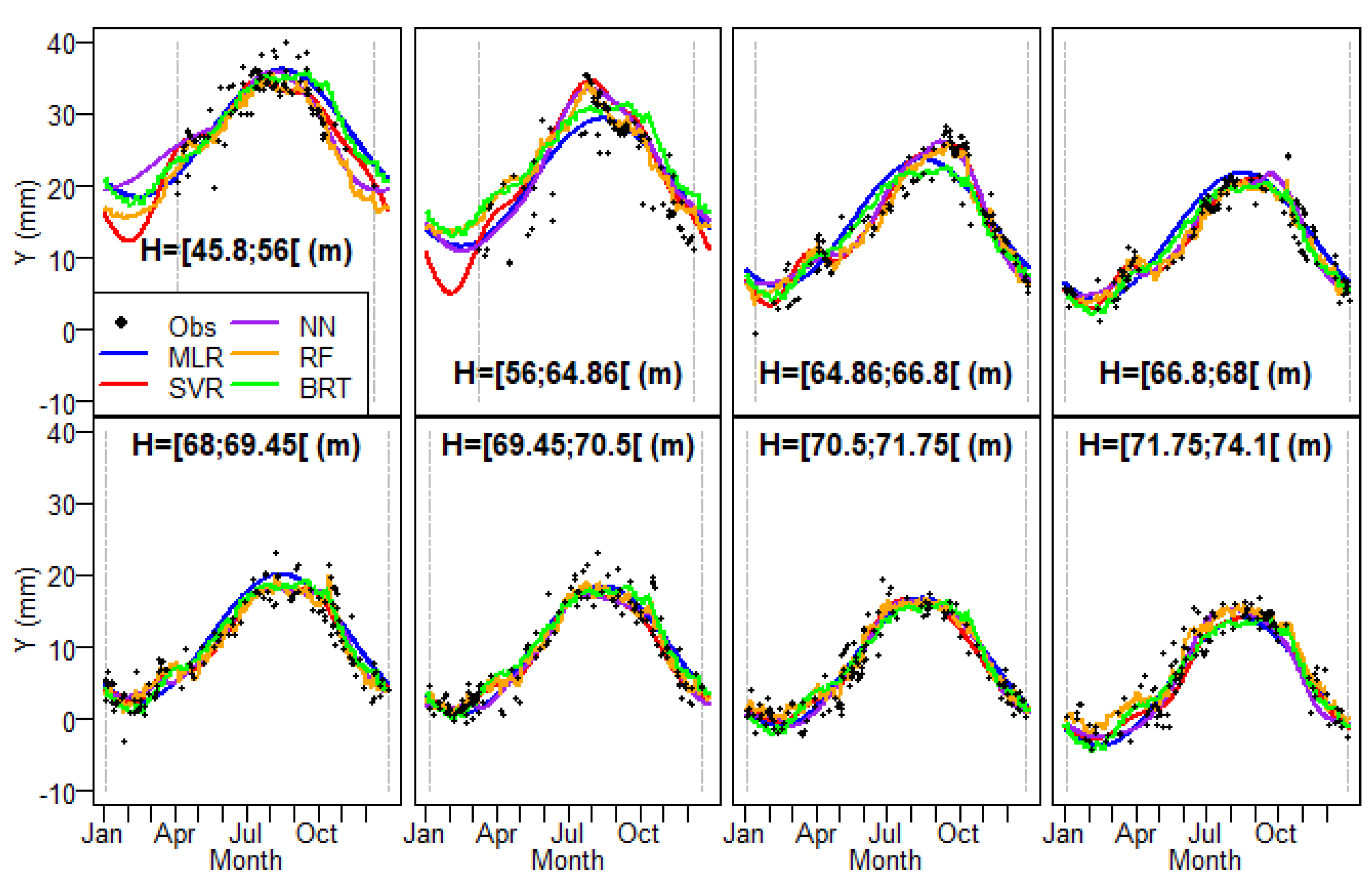
5.3. Step 3: Predictive Validation

The same methods used for historical data can be applied to the recent period of records, which was not used for model fitting.

The analysis of predictions for this period shall focus on detecting whether overfitting exists in ML models. First, prediction errors were computed (

Table 5. Performance parameters for the MLP, SVR, NN, RF and BRT models regarding the predicted set.

		MLR	SVR	NN	RF	BRT
mean($ϵ$)	(mm)	−0.61	−0.25	−0.29	−0.47	−0.52
mean($\left|ϵ\right|$)	(mm)	1.66	1.84	1.85	1.99	1.92
MAPE	(%)	38.41	34.85	37.26	46.88	58.21
${ϵ}_{max}$	(mm)	4.69	7.05	7.44	6.92	6.47
${ϵ}_{min}$	(mm)	0.00	0.01	0.01	0.00	0.02
RMSE	(mm)	2.02	2.39	2.40	2.51	2.42

). The highest prediction accuracy was obtained for MLR, though differences were slight.

The comparison between these results and those for the training set reveals a relevant difference between MLR and ML models: while the performance of MLR is better for the prediction set, all the others ML models featured lower accuracy. This result is reasonable and shows the tendency to overfitting of ML models. MLR is less flexible, which is a limitation under some circumstances (if more relevant inputs are involved or if response variables of a different nature need to be considered) and reduces the risk of overfitting. It can be concluded that training error is a good estimate of generalization capability for MLR but not for ML models. This implies that using a separated part of the training set to evaluate model accuracy is essential when ML models are used (e.g., NN), but not as critical for the MLR model.

The difference between accuracies on both datasets also depends on the distribution of the target variable in both sets. In the case study shown, the water level in the prediction period remains high. Consequently, the performance metrics of the models for this period correspond to their predictive capability for high water levels. In this case, since high levels were more frequent in the training set, model accuracy is also higher. Hence the overall prediction accuracy can be expected to be lower for all models. This should be taken into account in practice if the model is applied during a period of low hydrostatic load.

As in the training set, MAPE is high for all models for the same reason: a relatively low error for small target values may result in extremely high MAPE. As an example, the maximum MAPE for the MLR model is 560% for an observed displacement of 0.7 mm. This suggests that MAPE can be misleading when applied to certain target variables.

Figure 18 shows the time series of predictions and observations with the corresponding residuals. A first exploration of these plots may lead to the conclusion that all models have excessive variance: the time series of predictions is noisier than that of observations. However, it should be reminded that the reading frequency of the water level is higher than that of the displacements, and all predictions are shown in the plot. In addition, the time series of reservoir level is indeed noisy (maybe due to the daily variations of the water height in the reservoir). Taking these factors into consideration, the variance in predictions seems reasonable. In addition, similar variability can be observed for MLR and ML models. These conclusions were confirmed from the comparison between the standard deviation of the observations and that of the predictions from each model (see

Table 6. Standard deviation of predictions and observations for the training and predicted periods.

Time Series	Standard Deviation (mm)
	Training Set	Predicted Set
Observations	10.58	7.69
MLR	10.25	7.86
SVR	10.43	7.9
NN	10.45	7.97
BRT	10.35	8.12
RF	10.19	7.51

).

The plot of predictions vs. observations (Figure 19) shows no relevant differences to that for the training set. However, this kind of representation may be useful to check the performance and confirm that the prediction is within the domain of the horizontal displacements considered in the training set (vertical lines in the figure).

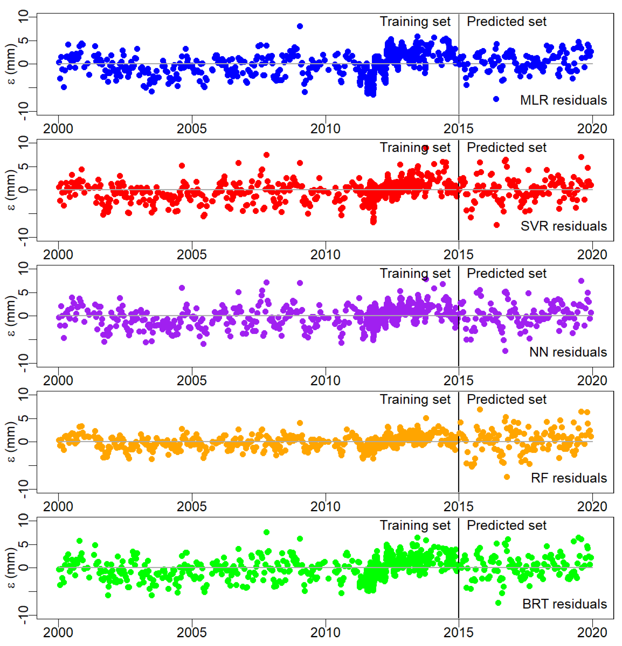
5.4. Step 4: Time Evolution of Residuals

The effect of time is often interpreted as the contribution of irreversible deformations to the displacements since, in principle, such term encompasses all effects not explained by the loads. This is the case of displacements in arch dams. In other typologies and response variables, other inputs may play a role and a more detailed analysis is recommended.

In the case study considered, preliminary tests on the MLR models showed no relevant irreversible effects. As a result, time was not considered as input in the models. However, further verification can be made even in models where time was considered negligible. Since model predictions are solely based on the external loads (temperature indirectly considered from the calendar day), the temporal evolution of the residuals may reveal unforeseen irreversible effects. This approach is similar to the analysis of the ”Corrected measurements” proposed by Guo et al. [65]: the difference between model predictions without time-dependent input and observed data can be considered as the evolution of the response of the dam for identical load conditions over time. It can be thus be expressed as presented in Equation (6):

$$CM = Y_{obs} - Y_{pred}$$

(6)

provided that time is not considered in the calculation of $Y_{pred}$.

Guo and co-authors also suggested fitting a linear model to the $CM$ to draw conclusions on the evolution of the dam behaviour with the Equation (7):

$$CM = a_0 + a_{1}t + ϵ$$

(7)

where t is the time.

The linear model can later be analysed to identify irreversible effects. This procedure was followed for all models. In all cases, the slope of the linear fit is positive and small, which might indicate a temporal evolution of the deformations toward the upstream direction, Figure 20. However, the fit of the linear model to the residuals is also poor for all models (R${}^2$ below 0.1), so no reliable conclusions can be drawn in this case.

5.5. Step 5: Comparison to Other Models

The interpretation of the structural behaviour through different models is fundamental to support an informed decision. This step was performed along with the four steps before, verifying that the presented ML models are suitable for the interpretation of the horizontal displacement analysed in the case study.

6. Conclusions and Final Remarks

In the day-to-day safety control of dams, data-based models are developed to analyse and predict structural dam behaviour (such as displacements in a concrete dam), considering main loads effects (such as the hydrostatic, temperature, and time effects).

The use of data-based models, namely based on $HST$ and $HTT$ approaches, using machine learning techniques, has had an interesting evolution in dam engineering. Worldwide, the increase in the day-to-day use of ML techniques is expected, mainly in large hydroelectric companies and entities responsible for dam safety control activities. In order to ensure that models are adequate, validation and verification of the models by specialists with expertise in dam engineering is necessary. In this work, the authors present several recommendations, with scientific and technical frameworks, to validate and verify ML models.

Based on the specificity of the dam safety control activities, five techniques to perform model validation and verification were proposed and applied to the following ML models: multiple linear regression, support vector machine, multilayer perceptron neural network, random forest, and regression trees. These five techniques were: historical data validation, sensitivity analysis, predictive validation, time evolution of the residuals, and comparison to other models. All the models presented showed to be suitable for the analysis and interpretation of the horizontal displacements presented in the case study. The proposed validation and verification of the ML models is based on five techniques that were never performed simultaneously. Sensitivity analysis is performed on all ML models, which is crucial for improving confidence in their day-to-day use.

Performing model validation and verification is part of the model development process. Our reflections and contributions are based on the article presented by Sargent [22] and on the authors’ experience acquired along years of activity in the field of dam safety control. They can be summarised as follows:

• Dams are made of, and founded on, materials whose properties change with time, so each data-based model has a limited lifetime (from a couple of months until several years) and a regular update of the parameters of the models based on “new data” is recommended. However, the model updating must be performed with data representing the typical (and acceptable) dam behaviour.
• Good data quality is necessary to obtain good ML models, but an adequate learning process is also necessary. The performance of the ML models is a consequence of the quality of data (directly related to the measurements uncertainties or even errors from the measuring process) and the suitability of the ML techniques adopted for the intended purpose (e.g., analysis and interpretation of the dam behaviour).
• ML models showed to be able to learn the pattern behaviour of the data (sometimes unseen from the users of the data). Some ML techniques are too prone to overfitting. However, an adequate generalization capacity can be achieved if a suitable learning strategy is adopted.
• Day-to-day dam safety activities based on data-based models are usually split into two parts: model development and operation. Each part uses different data (from the same source) recorded along time: the training and the prediction sets. However, these two sets are recorded measurements. So, regarding the historical data validation, two strategies can be performed: (i) use a part of the training set to validate the behaviour of the model or, in other words, to verify the adequacy and the generalization capacity of the model, and (ii) to use the own prediction set for this purpose (as usually verified in MLR because the shape of the terms adopted is well known in this field).
• To perform predictive validation is a routine activity of dam engineers. This process of forecast the structural response (based on known inputs) and compare to the observed response is fundamental to identify possible measurement errors or some change of the dam behaviour pattern observed before (namely on the training set) in order to draw conclusions regarding the safety state of the dam.
• The water level and the temperature variations are two important loads to be considered in the study of the dam behaviour, and their effect on horizontal displacements in concrete dams is well known. For this reason, performing sensitivity analysis in the model regarding these two loads is relevant to the model validation process. This is more important because one premise of the $HST$ approach (adopted in this work) is that the effects of the hydrostatic pressure, temperature, and time changes can be evaluated separately.
• The knowledge about the evolution of the residuals over time can provide beneficial information about how the reservoir-dam-foundation system changes. The properties of this system change over time. However, a slow time dependency variation is expected in most dams in normal exploitation. Evidence of trends may be, for example, related to changes in concrete proprieties due to alkalis-silica reactions.
• Using more than one predictive model and comparing the results is strongly recommended. This can also be useful if some of the models are based on the FEM, particularly when complex behaviour is observed or when the interpretation of the model suggests some potential anomaly.

ML methods have proven to be an interesting and suitable tool for developing data-based models, increasingly relevant mainly when the amount of information increases with the measurement history. Like any tool, it has to be used by specialists with a broad knowledge of how it works in order to obtain data-based models that satisfy the needs of the dam safety control activities. Within this continuous process, the validation and verification of the ML models adopted are key to having suitable models for reliable analysis and interpretation of the dam behaviour.

The proposed methodology for validation and verification of ML models can be applied to the prediction and analysis of other dam typologies and physical quantities, such as those related to the dynamic behaviour (e.g., frequencies modes) and hydro-mechanical phenomena (uplift pressure and seepage). This can increase the credibility of ML models in the dam engineering community and thus foster their widespread implementation.

References

1. ICOLD. Surveillance: Basic Elements in a Dam Safety Process; Bulletin Number 138; International Commission on Large Dams: Paris, France, 2009. [Google Scholar]
2. RSB. Regulation for the Safety of Dams; Decree-Law number 21/2018 of March 28; RSB: Porto, Portugal, 2018. (In Portuguese) [Google Scholar]
3. Lombardi, G. Advanced data interpretation for diagnosis of concrete dams. In Structural Safety Assessment of Dams; CISM: Udine, Italy, 2004. [Google Scholar]
4. Salazar, F.; Toledo, M.A.; Oñate, E.; Morán, R. An empirical comparison of machine learning techniques for dam behaviour modelling. Struct. Saf. 2015, 56, 9–17. [Google Scholar] [CrossRef] [Green Version]
5. Swiss Committee on Dams. Methods of analysis for the prediction and the verification of dam behaviour. In Proceedings of the 21st Congress of the International Commission on Large Dams, Montreal, Switzerland, 16–20 June 2003. [Google Scholar]
6. Leger, P.; Leclerc, M. Hydrostatic, Temperature, Time-Displacement Model for Concrete Dams. J. Eng. Mech. 2007, 133, 267–277. [Google Scholar] [CrossRef]
7. Mata, J. Interpretation of concrete dam behaviour with artificial neural network and multiple linear regression models. Eng. Struct. 2011, 33, 903–910. [Google Scholar] [CrossRef]
8. Simon, A.; Royer, M.; Mauris, F.; Fabre, J. Analysis and Interpretation of Dam Measurements using Artificial Neural Networks. In Proceedings of the 9th ICOLD European Club Symposium, Venice, Italy, 10–12 April 2013. [Google Scholar]
9. Ranković, V.; Grujović, N.; Divac, D.; Milivojević, N. Predicting piezometric water level in dams via artificial neural networks. Neural Comput. Appl. 2014, 24, 1115–1121. [Google Scholar] [CrossRef]
10. Granrut, M.; Simon, A.; Dias, D. Artificial neural networks for the interpretation of piezometric levels at the rock-concrete interface of arch dams. Eng. Struct. 2019, 178, 616–634. [Google Scholar] [CrossRef]
11. Rico, J.; Barateiro, J.; Mata, J.; Antunes, A.; Cardoso, E. Applying Advanced Data Analytics and Machine Learning to Enhance the Safety Control of Dams. In Machine Learning Paradigms: Applications of Learning and Analytics in Intelligent Systems 1; Tsihrintzis, G.A., Virvou, M., Sakkopoulos, E., Jain, L.C., Eds.; Springer International Publishing: Berlin/Heidelberg, Germany, 2019; pp. 315–350. [Google Scholar]
12. Li, M.; Wang, J. An Empirical Comparison of Multiple Linear Regression and Artificial Neural Network for Concrete Dam Deformation Modelling. Math. Probl. Eng. 2019, 2019, 7620948. [Google Scholar] [CrossRef] [Green Version]
13. Ren, Q.; Li, M.; Li, H.; Shen, Y. A novel deep learning prediction model for concrete dam displacements using interpretable mixed attention mechanism. Adv. Eng. Inform. 2021, 50, 101407. [Google Scholar] [CrossRef]
14. Chen, S.; Gu, C.; Lin, C.; Wang, Y.; Hariri-Ardebili, M.A. Prediction, monitoring, and interpretation of dam leakage flow via adaptative kernel extreme learning machine. Measurement 2020, 166, 108161. [Google Scholar] [CrossRef]
15. Kang, F.; Li, J.; Zhao, S.; Wang, Y. Structural health monitoring of concrete dams using long-term air temperature for thermal effect simulation. Eng. Struct. 2019, 180, 642–653. [Google Scholar] [CrossRef]
16. Qu, X.; Yang, J.; Chang, M. A Deep Learning Model for Concrete Dam Deformation Prediction Based on RS-LSTM. J. Sens. 2019, 2019, 4581672. [Google Scholar] [CrossRef]
17. Ranković, V.; Grujović, N.; Divac, D.; Milivojević, N. Development of support vector regression identification model for prediction of dam structural behaviour. Struct. Saf. 2014, 48, 142–149. [Google Scholar] [CrossRef]
18. Hariri-Ardebili, M.A.; Pourkamali-Anaraki, F. Support vector machine based reliability analysis of concrete dams. Soil Dyn. Earthq. Eng. 2018, 104, 276–295. [Google Scholar] [CrossRef]
19. Dai, B.; Gu, C.; Zhao, E.; Qin, X. Statistical model optimized random forest regression model for concrete dam deformation monitoring. Struct. Control Health Monit. 2018, 25, e2170. [Google Scholar] [CrossRef]
20. Salazar, F.; Toledo, M.A.; Oñate, E.; Suárez, B. Interpretation of dam deformation and leakage with boosted regression trees. Eng. Struct. 2016, 119, 230–251. [Google Scholar] [CrossRef] [Green Version]
21. Salazar, F.; Morán, R.; Toledo, M.Á.; Oñate, E. Data-Based Models for the Prediction of Dam Behaviour: A Review and Some Methodological Considerations. Arch. Comput. Methods Eng. 2017, 24, 1–21. [Google Scholar] [CrossRef] [Green Version]
22. Sargent, R. Verification and validation of simulation models. In Proceedings of the 2010 Winter Simulation Conference, Baltimore, MD, USA, 5–8 December 2010. [Google Scholar]
23. Schweinsberg, M.; Feldman, M.; Staub, N.; van den Akker, O.R.; van Aert, R.C.M.; van Assen, M.A.L.M.; Liu, Y.; Althoff, T.; Heer, J.; Kale, A.; et al. Same data, different conclusions: Radical dispersion in empirical results when independent analysts operationalize and test the same hypothesis. Organ. Behav. Hum. Decis. Process. 2021, 165, 228–249. [Google Scholar] [CrossRef]
24. Childers, C.P.; Maggard-Gibbons, M. Same data, opposite results? A call to improve surgical database research. JAMA Surg. 2020, 156, 219–220. [Google Scholar] [CrossRef] [PubMed]
25. Mitchell, T.M. Machine Learning; McGraw Hill: Burr Ridge, IL, USA, 1997; Volume 45, pp. 870–877. [Google Scholar]
26. Mata, J.; Leitao, N.S.; de Castro, A.T.; da Costa, J.S. Construction of decision rules for early detection of a developing concrete arch dam failure scenario. A discriminant approach. Comput. Struct. 2014, 142, 45–53. [Google Scholar] [CrossRef] [Green Version]
27. Salazar, F.; Conde, A.; Vicente, D.J. Identification of Dam behaviour by Means of Machine Learning Classification Models. In Lecture Notes in Civil Engineering, Proceedings of the ICOLD International Benchmark Workshop on Numerical Analysis of Dams, ICOLD-BW, Milan, Italy, 9–11 September 2019; Springer: Cham, Switzerland, 2019; Volume 91, pp. 851–862. [Google Scholar]
28. Willm, G.; Beaujoint, N. Les méthodes de surveillance des barrages au service de la production hydraulique d’Electricité de France-Problèmes ancients et solutions nouvelles. In Proceedings of the 9th ICOLD Congres, Istanbul, Turkey, 4–8 September 1967; Volume III, pp. 529–550. (In French). [Google Scholar]
29. Montgomery, D.C.; Runger, G.C. Applied Statistics and Probability for Engineers; John Wiley & Sons, Inc.: Hoboken, NJ, USA, 1994. [Google Scholar]
30. Johnson, R.A.; Wichern, D.W. Applied Multivariate Statistical Analysis, 4th ed.; Prentice Hall: Hoboken, NJ, USA, 1998. [Google Scholar]
31. Kutner, M.H.; Nachtsheim, C.J.; Neter, J.; Li, W. Applied Linear Statistical Models, 5th ed.; McGraw-Hill Higher Education: New York, NY, USA, 2004. [Google Scholar]
32. Hastie, T.; Tibshirani, R.; Firedman, J. The Elements of Statistical Learning-Data Mining, Inference, and Prediction, 2nd ed.; Springer: Berlin/Heidelberg, Germany, 2009. [Google Scholar]
33. Stojanovic, B.; Milivojevic, M.; Milivojevic, N.; Antonijevic, D. A self-tuning system for dam behaviour modeling based on evolving artificial neural networks. Adv. Eng. Softw. 2016, 97, 85–95. [Google Scholar] [CrossRef]
34. Kao, C.Y.; Loh, C.H. Monitoring of long-term static deformation data of Fei-Tsui arch dam using artificial neural network-based approaches. Struct. Control Health Monit. 2013, 20, 282–303. [Google Scholar] [CrossRef]
35. Bishop, C.M. Neural Networks for Pattern Recognition; Oxford University Press: New York, NY, USA, 1995. [Google Scholar]
36. Breiman, L. Random forests. Mach. Learn. 2001, 45, 5–32. [Google Scholar] [CrossRef] [Green Version]
37. Díaz-Uriarte, R.; Alvarez de Andrés, S. Gene selection and classification of microarray data using random forest. BMC Bioinform. 2006, 7, 20. [Google Scholar] [CrossRef] [Green Version]
38. Moguerza, J.M.; Muñoz, A. Support vector machines with applications. Stat. Sci. 2006, 21, 322–336. [Google Scholar] [CrossRef] [Green Version]
39. Smola, A.J.; Schölkopf, B. A tutorial on support vector regression. Stat. Comput. 2004, 14, 199–222. [Google Scholar] [CrossRef] [Green Version]
40. Fisher, W.D.; Camp, T.K.; Krzhizhanovskaya, V.V. Anomaly detection in earth dam and levee passive seismic data using support vector machines and automatic feature selection. J. Comput. Sci. 2017, 20, 143–153. [Google Scholar] [CrossRef]
41. Cheng, L.; Zheng, D. Two online dam safety monitoring models based on the process of extracting environmental effect. Adv. Eng. Softw. 2013, 57, 48–56. [Google Scholar] [CrossRef]
42. Hariri-Ardebili, M.A.; Salazar, F. Engaging soft computing in material and modeling uncertainty quantification of dam engineering problems. Soft Comput. 2020, 24, 11583–11604. [Google Scholar] [CrossRef]
43. Friedman, J. Greedy function approximation: A gradient boosting machine. Ann. Stat. 2001, 29, 1189–1232. [Google Scholar] [CrossRef]
44. Elith, J.; Leathwick, J.R.; Hastie, T. A working guide to boosted regression trees. J. Anim. Ecol. 2008, 77, 802–813. [Google Scholar] [CrossRef]
45. Leathwick, J.; Elith, J.; Francis, M.; Hastie, T.; Taylor, P. Variation in demersal fish species richness in the oceans surrounding New Zealand: An analysis using boosted regression trees. Mar. Ecol. Prog. Ser. 2006, 321, 267–281. [Google Scholar] [CrossRef] [Green Version]
46. Mata, J.; Tavares de Castro, A.; Sá da Costa, J. Quality control of dam monitoring measurements. In Proceedings of the 8th ICOLD European Club Symposium, Graz, Austria, 22–23 September 2010. [Google Scholar]
47. Mata, J.; Martins, L.; Tavares de Castro, A.; Ribeiro, A. Statistical quality control method for automated water flow measurements in concrete dam foundation drainage systems. In Proceedings of the 18th International Flow Measurement Conference, Lisbon, Portugal, 26–28 June 2019. [Google Scholar]
48. Mata, J.; Martins, L.; Ribeiro, A.; Tavares de Castro, A.; Serra, C. Contributions of applied metrology for concrete dam monitoring. In Proceedings of the Hydropower’15, ICOLD, Stavanger, Norway, 14–19 June 2015. [Google Scholar]
49. Sun, X.Y.; Newham, L.T.H.; Croke, B.F.W.; Norton, J.P. Three complementary methods for sensitivity analysis of a water quality model. Environ. Model. Softw. 2012, 37, 19–29. [Google Scholar] [CrossRef]
50. Song, X.; Zhang, J.; Zhan, C.; Xuan, Y.; Ye, M.; Xu, C. Global sensitivity analysis in hydrological modeling: Review of concepts, methods, theoretical framework, and applications. J. Hydrol. 2015, 523, 739–757. [Google Scholar] [CrossRef] [Green Version]
51. Borgonovo, E.; Plischke, E. Sensitivity analysis: A review of recent advances. Eur. J. Oper. Res. 2016, 248, 869–887. [Google Scholar] [CrossRef]
52. Pianosi, F.; Beven, K.; Freer, J.; Hall, J.W.; Rougier, J.; Stephenson, D.B.; Wagener, T. Sensitivity analysis of environmental models: A systematic review with practical workflow. Environ. Model. Softw. 2016, 79, 214–232. [Google Scholar] [CrossRef]
53. Pang, Z.; O’Neill, Z.; Li, Y.; Niu, F. The role of sensitivity analysis in the building performance analysis: A critical review. Energy Build. 2020, 209, 142–149. [Google Scholar] [CrossRef]
54. Douglas-Smith, D.; Iwanaga, T.; Croke, B.F.W.; Jakeman, A.J. Certain trends in uncertainty and sensitivity analysis: An overview of software tools and techniques. Environ. Model. Softw. 2020, 124, 142–149. [Google Scholar] [CrossRef]
55. R Core Team. R: A Language and Environment for Statistical Computing; R Foundation for Statistical Computing: Vienna, Austria, 2021. [Google Scholar]
56. RStudio Team. RStudio: Integrated Development Environment for R; R Studio, Inc.: Boston, MA, USA, 2019. [Google Scholar]
57. Venables, W.N.; Ripley, B.D. Modern Applied Statistics with S, 4th ed.; Springer: New York, NY, USA, 2002; ISBN 0-387-95457-0. [Google Scholar]
58. Liaw, A.; Wiener, M. Classification and Regression by randomForest. R News 2002, 2, 18–22. [Google Scholar]
59. Therneau, T.; Atkinson, B. rpart: Recursive Partitioning and Regression Trees; R Package Version 4.1-15; R Foundation for Statistical Computing: Vienna, Austria, 2019. [Google Scholar]
60. Peters, A.; Hothorn, T. ipred: Improved Predictors; R Package Version 0.9-11; R Foundation for Statistical Computing: Vienna, Austria, 2021. [Google Scholar]
61. Slowikowski, K. ggrepel: Automatically Position Non-Overlapping Text Labels with ‘ggplot2’; R Package Version 0.9.1; R Foundation for Statistical Computing: Vienna, Austria, 2021. [Google Scholar]
62. Greenwell, B.; Boehmke, B.; Cunningham, J. gbm: Generalized Boosted Regression Models; R Package Version 2.1.8; CRAN: Vienna, Austria, 2020. [Google Scholar]
63. Muralha, A.; Couto, L.; Oliveira, M.; Dias da Silva, J.; Alvarez, T.; Sardinha, R. Salamonde dam complementary spillway. Design, Hydraulic model and ongoing works. In Proceedings of the Dam World Conference, Lisbon, Portugal, 21–25 April 2015. [Google Scholar]
64. Cortez, P.; Embrechts, M. Using sensitivity analysis and visualization techniques to open black box data mining models. Inf. Sci. 2013, 225, 1–17. [Google Scholar] [CrossRef] [Green Version]
65. Guo, X.; Baroth, J.; Dias, D.; Simon, A. An analytical model for the monitoring of pore water pressure inside embankment dams. Eng. Struct. 2018, 160, 356–365. [Google Scholar] [CrossRef]
Figure 1. Supervised and unsupervised learning approaches.
Water 13 02717 g001
Figure 2. Main machine learning techniques used in dam safety assessment context.
Water 13 02717 g002
Figure 3. General scheme for fitting and applying predictive models based on monitoring data.
Water 13 02717 g003
Figure 4. Simplified version of the modelling process for dam engineering, adapted from [22].
Water 13 02717 g004
Figure 5. Proposed techniques for the verification and validation of ML models for dam behaviour interpretation.
Water 13 02717 g005
Figure 6. Salamonde dam: Upstream and downstream dam faces and pendulum distribution.
Water 13 02717 g006
Figure 7. Radial displacements in FP3/5–277.07 m and reservoir water level along time.
Water 13 02717 g007
Figure 8. Water height from 2000 to 2019, by month (training set: from 2000 to 2014 and predicted set: from 2015 to 2019).
Water 13 02717 g008
Figure 9. Water height from 2000 to 2019, in polar coordinate system, by month (training set: from 2000 to 2014 and predicted set: from 2015 to 2019).
Water 13 02717 g009
Figure 10. Radial displacements in FP3/5–277.07 m from 2000 to 2019 by month (training set: from 2000 to 2014 and predicted set: from 2015 to 2019).
Water 13 02717 g010
Figure 11. Radial displacements in FP3/5–277.07 m from 2000 to 2019 in polar coordinate system, by month (training set: from 2000 to 2014 and predicted set: from 2015 to 2019).
Water 13 02717 g011
Figure 12. Workflow of the proposed techniques for the verification and validation of ML models for dam behaviour interpretation.
Water 13 02717 g012
Figure 13. Measurements of the training set and output of the Machine Learning models for the horizontal upstream-downstream displacements at FP3/5–277.07 m base, block GH.
Water 13 02717 g013
Figure 14. ML model residuals distribution for the training data.
Water 13 02717 g014
Figure 15. ML model values vs measurements of radial displacements in FP5/5–277.07 m from 2000 to 2014 (training data). The vertical lines are the maximum and minimum measured values obtained during the training set.
Water 13 02717 g015
Figure 16. Sensitivity analysis due to the hydrostatic effect for Machine Learning model results based on the training data. The vertical lines are the maximum and minimum measured values obtained during the training set.
Water 13 02717 g016
Figure 17. Sensitivity analysis due to the thermal effect for Machine Learning model results based on the training data. The vertical lines are the maximum and minimum measured values obtained during the training set.
Water 13 02717 g017
Figure 18. Measurements of the predicted set and output of the Machine Learning models for the horizontal upstream-downstream displacements at FP3/5–277.07 m base, block GH.
Water 13 02717 g018
Figure 19. ML Model values vs measurements of radial displacements in FP5/5–277.07 m from 2015 to 2019 (predicted data). The vertical lines are the maximum and minimum measured values obtained during the training set.
Water 13 02717 g019
Figure 20. Residuals along the training and the predicted sets.
Water 13 02717 g020