Article

A Multigrid Dynamic Bidirectional Coupled Surface Flow Routing Model for Flood Simulation

1
State Key Laboratory of Hydroscience and Engineering, Department of Hydraulic Engineering, Tsinghua University, Beijing 100084, China
2
School of Hydraulic Engineering, Faculty of Infrastructure Engineering, Dalian University of Technology, Dalian 116024, China
*
Authors to whom correspondence should be addressed.
Water 2021, 13(23), 3454; https://doi.org/10.3390/w13233454
Submission received: 17 October 2021 / Revised: 23 November 2021 / Accepted: 2 December 2021 / Published: 5 December 2021
(This article belongs to the Special Issue Urban Flood Model Developments and Flood Forecasting)

Abstract

:
Surface flow routing is an important component in hydrologic and hydrodynamic research. Based on a literature review and comparing the different coupling models (the hydrologic model and hydrodynamic model), a multigrid dynamic bidirectional coupled surface flow routing model (M-DBCM), consisting of diffusion wave equations (DWEs) and shallow water equations (SWEs), is proposed herein based on grids with different resolutions. DWEs were applied to obtain runoff routing in coarse grid regions to improve the computational efficiency, while the DWEs and SWEs were bidirectionally coupled to detail the flood dynamics in fine grid regions to obtain good accuracy. In fine grid zones, the DWEs and SWEs were connected by an internal moving boundary, which ensured the conservation of mass and momentum through the internal moving boundary. The DWEs and SWEs were solved by using the time explicit scheme, and different time steps were adopted in regions with different grid sizes. The proposed M-DBCM was validated via three cases, and the results showed that the M-DBCM can effectively simulate the process of surface flow routing, which had reliable computational efficiency while maintaining satisfactory simulation accuracy. The rainfall runoff in the Goodwin Creek Watershed was simulated based on the proposed M-DBCM. The results showed that the discharge hydrographs simulated by the M-DBCM were closer to the measured data, and the simulation results were more realistic and reliable, which will be useful in assisting flood mitigation and management.

1. Introduction

Surface flow routing, consisting of overland and channel flow routing, refers to the process in which a precipitation-generated surface runoff moves over the land surface from the source to an outlet. An accurate description of surface flow routing plays an important role in a variety of hydrologic, hydrodynamic, and ecological problems, such as flood routing, rainfall runoff modeling, sediment transport, pollutant convection diffusion, and so on [1,2]. In particular, the consequences of flow-related events have recently been described according to abnormal meteorological phenomena, occurring possibly due to climate change, especially extreme flooding events, which have many adverse effects on human life and damage of property [3]. Therefore, simulating the surface flow routing is key to minimizing the potential human and property damage from floods.
Many researchers have studied rainfall–runoff mechanisms and ways to reduce the loss caused by floods, using physically-based hydrologic and hydrodynamic models for simulations [4,5,6,7]. However, the hydrologic model has been widely used for overland flows but rarely expanded to the simulation of flood propagation processes. The hydrodynamic model has played a major role in simulating inundation processes, which have been computationally prohibitive for large-scale applications. Consequently, coupling models have been developed to combine the advantages of the hydrologic and hydrodynamic models to simulate surface flow routing accurately, which can be classified into the external coupling model and internal coupling model [8], as shown in Figure 1. However, these coupling models have two main disadvantages, resulting in inaccurate surface flow routing simulation.
The first disadvantage is the coupling manners. The hydrologic model and hydrodynamic model undergo one-way coupling in most of the existing coupling models, and the boundary positions of the hydrodynamic model are also fixed. In the external coupling model, the hydrographs obtained from the hydrologic model feed the hydrodynamic model and are calculated at the second stage. For example, Li et al. [9] proposed an external coupling model where the TOPMODEL (TOPography-based hydrological MODEL, developed by Lancaster University, Lancaster, UK) was employed to obtain the flood hydrograph, and Mike Flood was used to simulate the floodplain inundation, but there was less accuracy in the estimation of the low flows in tributaries. An external coupling model connecting SWAT (Soil and Water Assessment Tool) and GEMSS (Generalized Environmental Modeling System for Surface waters, a 3D time-dependent hydrodynamic model) was developed by Dargahi and Setegn [10], which was used to simulate flooding in the Tana Basin, and similar methods were used in studies of other catchments [11,12,13,14,15,16,17].
Since the flow information was transferred one way from the hydrologic model to the hydrodynamic model, the external coupling model could not capture the mutual interaction between runoff production and flood inundation, which was not in line with the reality of the situation. What is more, due to the fixed position of the coupling boundary between the hydrologic model and hydrodynamic model and the limited number of coupling boundary points, the runoff generation on both sides of the river was transferred to the upstream of the main stream or tributaries of the river network, resulting in an error in the peak flow rate of the boundary points, and a reduction in the calculation accuracy. Mass conservation of water through the coupling interface also could not be guaranteed.
Unlike in the external coupling model, discharge information can be exchanged between the hydrologic and hydrodynamic models in the internal coupling model; that is, the hydrological process affects hydrodynamic processes, and the hydrodynamic process also affects the hydrological process. The coupling of Mike SHE (Système Hydrologique Européen, a distributed hydrological model) and Mike11 is a typical example of the coupling of the hydrologic and 1D hydrodynamic model [18,19]. The flow discharge rate obtained from the hydrologic model was treated as the mass source of the 1D hydrodynamic model, while the water depth calculated in the 1D hydrodynamic model was fed back to the hydrologic model [20]. However, as the 1D hydrodynamic model was employed in this coupling model, it could not provide enough 2D flood inundation information. The 2D hydrodynamic model was needed for the inundation prediction.
Therefore, the coupling of the hydrologic model and 1D and 2D hydrodynamic model was developed to simulate the flood inundation information more accurately [21,22,23], where the hydrologic model was first coupled with the 1D hydrodynamic model, and then the 1D and 2D hydrodynamic models were dynamically coupled in a bidirectional way, as an indirect dynamic coupling of the hydrologic model and 2D hydrodynamic model. For instance, Mike SHE and Mike11 were coupled to form Mike Urban, and Mike11 and Mike21 were dynamically coupled to form a model called Mike Flood. The indirect coupling between Mike SHE and Mike21 can be realized by coupling Mike Urban and Mike Flood, and Mike11 was the connection channel between Mike SHE and Mike21. Some other similar models for indirect coupling of the hydrologic and 2D hydrodynamic models can be found in [21,24]. The hydrologic model was not directly linked with the 2D hydrodynamic model, and this was inconsistent with actual flood conditions. In reality, the runoff may flow into both the 1D channel and 2D inundation regions simultaneously, and the hydrologic model and 2D hydrodynamic model should be linked directly. It is undeniable that 1D channel flow has an effect on the formation of the 2D inundation region, but the rainstorm can directly form a 2D inundation region in low-lying areas. Direct dynamic coupling of the distributed hydrologic model and 2D hydrodynamic model can reflect the formation of a 2D inundation region more realistically. The dynamic bidirectional coupling of the distributed hydrologic model and the local 2D hydrodynamic model has been paid much attention [25]. However, the problems of determining the coupling boundary and calculating the flux of water and momentum through the coupling boundary have not yet been solved.
Another problem of the coupling models is the computational efficiency, which is more evident in the full 2D hydrodynamic model. In the full 2D hydrodynamic model, the runoff generation is only calculated in the hydrologic model, while the overland flow movement and inundation processes are all calculated in the hydrodynamic model [26] which increases the difficulties of data preprocessing and decreases the computing efficiency. Moreover, its numerical stability problems need to be paid more attention to in the thin-layer water regions [27]. For example, Kim et al. [28] developed a TRIBS-OFM (Triangulated Irregular Network–Based Real-Time Integrated Basin Simulator and Overland Flow Model), where the hydrologic model was only used to calculate rainfall generation and the 2D hydrodynamic model was used to simulate the slope flow and flood-inundation, which showed good calculation accuracy but low calculation efficiency. Some other similar models for the full 2D hydrodynamic model can be found in [6,26,27]. Since the 2D hydrodynamic equation needs to be solved in most areas, this inevitably leads to an increase in the required computational power, especially if results need to be computed at a fine spatial resolution, and its numerical stability problems need to be paid more attention in the thin-layer water regions [27].
It is noted that the flood inundation region is only a part of the watershed. The 2D hydrodynamic model can be solved in the locally inundated region to ensure calculation accuracy, and the hydrologic model can be solved in the non-inundated region to save on calculation time and improve numerical stability. That is, different models were used in different spatial regions. Therefore, it is necessary to develop suitable coupling methods between the hydrologic model and hydrodynamic model. In this study, in order to improve the calculation efficiency while maintaining accuracy, following the previous study of our research group, a multigrid dynamic bidirectional coupled surface flow routing model (M-DBCM) that consisted of SWEs and DWEs is proposed based on grids with different resolutions. In M-DBCM, the SWEs and DWEs were solved synchronously, which ensured the conservation of mass and momentum flux on the coupled boundary, and therefore, the numerical accuracy was improved compared with the external coupling model. The computational domain was divided into zones with different gird sizes in M-DBCM. The coarse grid was used for solving DWEs for less flood-prone areas, thus not unnecessarily increasing computational costs, while the DWEs were spatially coupled in a two-way manner with the SWEs on fine grid regions, allowing for the exchange of information throughout the entire computational domain. The M-DBCM can improve both the computational efficiency and the numerical stability in comparison with the fully 2D hydrodynamic model. Finally, three cases were used to verify the performance of the proposed model, and the rainfall runoff in the Goodwin Creek Watershed was simulated.

2. Methods

In M-DBCM, the computational domain was divided into sub-regions with different grid sizes. In coarse grid regions, DWEs were used to calculate the rainfall runoff, while the simulation on fine grid zones was the same as in DBCM, a dynamic bidirectional coupling model developed by our research group [29]. That is, a water depth threshold was used to determine the calculation regions of the SWEs and DWEs. If the water depth was greater than the threshold, the SWEs were used to calculate the runoff, while in regions in which the water depth was lower than the threshold, the algorithm applying the SWEs to calculate the flow movement in the thin-layer water regions had a numerical instability problem, and therefore, the DWEs were used to simulate the flows in the thin-layer water regions.

2.1. Zone Partition and Grid System

A structured grid was applied to discretize the computational regions, as it has the advantages of simplicity and intuitiveness, and a highly accurate scheme can be built with ease. A uniform grid was used to divide the computational domain in the previous DBCM. The computational domain was divided into the SWE regions and DWE regions according to the water depth threshold. The regions were considered as DWE regions if the water depth was lower than the threshold, where the DWEs were used to calculate runoff, while the regions were defined as SWE regions if the water depth was higher than the threshold, where the SWEs were used to calculate runoff. These two regions were connected by an internal moving boundary. However, for the watershed flood prediction, the DWE regions were much larger than the SWE regions, and it was not necessary to use the same fine grid in both regions. Therefore, the application of multigrid technology can further save computing time, which resulted in the present M-DBCM.
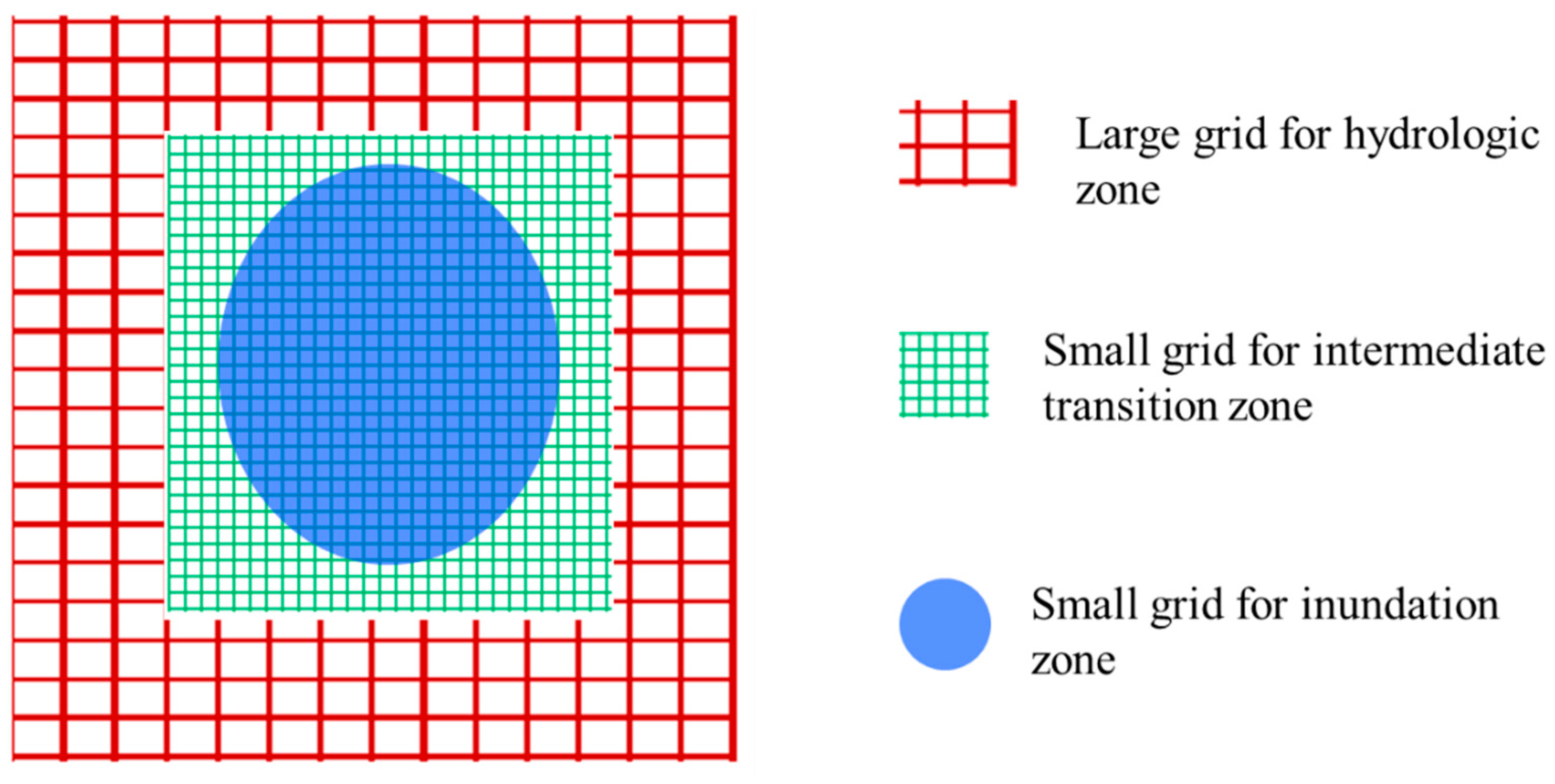
In the proposed M-DBCM, as shown in Figure 2, the computational regions were divided into zones with different grid sizes. The coarse and fine mesh zones were estimated in advance based on the topographic elevation map. The DWEs were used to calculate the runoff routing in coarse grid regions that were not vulnerable to floods. Within the fine grid regions, the DWE regions and SWE regions were determined according to the water depth threshold. In regions with a water depth above the threshold, SWEs were used for hydrodynamic calculations, while in the zones with a water depth below the threshold, DWEs were used for runoff routing calculations.
As shown in Figure 2, connecting lines were formed between the coarse grid and fine grid. The position of the grid size variation line was fixed, which facilitated data exchange among different grids. In the fine grid regions, the coupled moving boundary between the SWEs and DWEs was varied according to the water depth, and the mass and momentum conservation through the internal moving boundary was able to be satisfied. The application of the multigrid technique made the M-DBCM more efficient.

2.2. Description of the Coupled Surface Flow Routing Model

2.2.1. Runoff Generation

The runoff generation of a catchment involves precipitation and infiltration. The precipitation was interpolated from rainfall station data by inverse distance interpolation, which indicated that the hydrological similarity of the two points increased with the decrease in the distance, and the calculation formula was as follows:
R n = i = 1 N λ i R i
where R n is the value (mm/d) to be estimated; R i is the rainfall data (mm/d) of the ith hydrological station; λ i is the interpolation coefficient of the ith hydrological station, and N represents the number of hydrological stations.
Infiltration was calculated using the Green-Ampt equation, and the formulation is shown as follows:
f p = K s ( 1 + ( θ s θ i ) S a F c )
where f p is the infiltration rate (m/s); K s is the hydraulic conductivity (m/s); S a is the average effective suction of the wetting front (mm); θ s and θ i are the saturated and initial soil moisture content (%), respectively; and F c is the cumulative infiltration (mm).

2.2.2. Surface Flow Routing

Shallow Water Equations

The SWEs are the most widely used in hydrodynamic models for flood simulation [27]. Neglecting the Coriolis force, wind resistance, and viscosity, the equations consist of the continuity equation and momentum equations, which can be written as:
U t + F x + G y = S
where U, F, and G are the vectors of the conserved flow variables and fluxes along the x and y directions, respectively; and S is the sources vector including the bed slope, frictional force, and mass source of the continuity equation. These vectors are expressed as:
U = [ h , h u , h v ] T ,   F = [ h u , h u 2 + g h 2 / 2 , h u v ] T G = [ h v , h u v , h v 2 + g h 2 / 2 ] T S = [ Q m , g h z x g C 2 u u 2 + v 2 , g h z y g C 2 v u 2 + v 2 ] T
where u and v are velocities in the x and y directions (m/s), respectively, h is the water depth (m); Q m is the value that is equal to the rainfall rate minus the infiltration rate (m/s); g is gravity acceleration (m/s2); z is the elevation (m), and C is the Chezy coefficient, representing roughness.
A Godunov-type fine volume scheme with an HLLC (Harten-Lax-van Leer contact) approximate Riemann solver [28,29,30] was adopted to discretize the SWEs on a structured grid, and the second-order accuracy in spatial discretization was obtained [24,31]. The discretized form of the governing equations can be written as:
U i n + 1 = U i n Δ t A m = 1 N [ F ( U n ) m d y m G ( U n ) m d x m ] + Δ t S ( U i n )
where n and n + 1 are the variables at the current and next time step, respectively; Δ t is the time step; A is the cell area; i is the index of a cell; N is the number of edges of the cell, and for quadrilateral meshes, m = 1,2,3,4; F ( U n ) m and G ( U n ) m are the vectors of the Riemann flux, calculated by solving a local Riemann problem normal to the edge m; U is the vectors of conservative variables on the edge m, and S ( U i n ) is the source term.
However, the algorithm applying the SWEs to calculate the flow movement in very shallow overland showed numerical instability [28], and it can take more time to solve SWEs in whole regions. In order to overcome the problem of numerical instability and improve calculation efficiency, the SWEs could be solved in local regions, which is one of the innovations of this study.

Diffusion Wave Equations

In order to describe the flow movement more accurately, especially in very shallow overland, the DWEs were used to calculate the runoff routing, which consisted of the mass conservation equation and momentum equations, as follows:
h t + q x x + q y y = Q m
Q x = A x R x 0.67 S x 0.5 n
Q y = A y R y 0.67 S y 0.5 n
where q x and q y are the unit discharges in the x and y directions (m2/s), respectively; h refers to the water depth (m); Q x and Q y denote the flow rate in the directions of x and y (m3/s), respectively; A refers to the flow area (m2); R is the hydraulic radius (m); S is the water level gradient, and n is the roughness coefficient.
In solving the DWEs, the flow velocity only depended on the local water level gradient and roughness, and the water depth was determined through water volume balance and discharge from the neighbor grids. The possible flow at one cell was linked to two adjacent cells at each time step. The solution formula can be further written as:
Q i = w h 5 / 3 S i n ( S i 2 + S j 2 ) 0.25 ,   Q j = w h 5 / 3 S j n ( S i 2 + S j 2 ) 0.25
where S i = η i , j η i ± 1 , j w , S j = η i , j η i , j ± 1 w ,
h i = η i , j max ( z i , j , z i ± 1 , j )
h j = η i , j max ( z i , j , z i , j ± 1 )
where w is the size of the grid (m); S i and S j are the water level slopes in x and y directions; h i and h j refer to the effective depths in x and y directions, and η i , j and z i , j are the water surface level and the ground elevation, respectively.
The effective depth in a grid cell was calculated as follows:
h = h i S i 2 h j S j 2 S i 2 + S j 2
where h is the effective depth of a grid cell.
The change in water depth in each grid cell was calculated as follows:
Δ h = ( Q i n i , j Q o u t i , j Q m ) Δ t Δ x Δ y
where Q i n is the inflow of a grid cell and Q o u t is the outflow of a grid cell.

2.3. Coupling Strategies

2.3.1. Multigrid and Variable Interpolation

In M-DBCM, with sudden changes in mesh sizes, additional nodes need to perform the differential calculations, and data interchange needs to be considered carefully. In the proposed M-DBCM, since the size of the coarse grid was an integer multiple of the size of the fine grid, the coarse grid had corresponding nodes on the fine grid side, and differential calculations could be performed normally. For the calculation of fine grids, the differential calculation had no corresponding nodes on the coarse grid side. Therefore, interpolation functions were constructed to ensure the calculation proceeded normally. The coupling strategies between the coarse grid and fine grid in the fixed boundary are shown in Figure 3. In this figure, P d 1 and P d 2 were considered as shared nodes, and the water depth and flow velocity between different meshes were transmitted directly, while P w 2 , P w 3 , , P w n 1 were defined as unshared nodes. The water depth and flow velocity could be obtained by linear interpolation of the shared nodes P d 1 and P d 2 .
In the areas with the fine grid, according to the water depth threshold, the regions that were calculated using SWEs or DWEs were determined before every time step. The SWEs and DWEs were dynamically coupled, and both algorithms were solved simultaneously within each time step. The conservations of mass and momentum on the internal moving boundary between the SWEs and DWEs were guaranteed by using the cell-centered finite volume (CCFV) scheme, and the position of the coupling boundary was not fixed but rather was time-dependent. The dynamic two-way coupling process of the SWEs and DWEs can be found in [29]. In the proposed M-DBCM, the calculation results of the DWEs affected the calculation of the SWEs, and the results of the SWEs also affected the DWEs, taking into account effects due to overflowing in the floodplain and backwater effects at confluences.
The coupling algorithm between the SWEs and DWEs based on the coarse and fine grids is presented in Figure 4.
In Figure 4, Δ t d is the time step on the coarse grid, while Δ t w is the time step on the fine grid. n represents the number of cycles on the coarse grid, while k represents the number of cycles on the fine grid. h d and h w are the water depth on the coarse grid and fine grid, respectively. u d and v d are the flow velocity along the x and y directions on the coarse grid, respectively, while u w and v w are the flow velocity along the x and y directions on the fine grid, respectively. T is the total simulation time. The coupling process between the SWEs and DWEs based on different gird sizes was as follows:
  • Step 1: The DWEs were used to simulate rainfall runoff on the coarse grid to obtain the water depth h d n , k and flow velocity u d n , k , v d n , k .
  • Step 2: The information, such as water depth and velocity, was updated from the coarse grid to fine grid. The water depth and flow velocity in shared nodes could be transmitted directly between different meshes, and linear interpolation was used to calculate the water depth and velocity in unshared nodes. Therefore, the water depth h w n , k and velocity u w n , k , v w n , k on the coupling boundary between the coarse gird and fine grid were determined to drive the simulation on the fine grid.
  • Step 3: The dynamic two-way coupling of the DWEs and SWEs was developed on the fine grid to obtain the water depth h w n , k + 1 and velocity u w n , k + 1 , v w n , k + 1 .
  • Steps 2 and 3 were repeated k times to obtain the data for the calculation of the DWEs at the next time on the coarse grid.
  • Step 4: The water depth h d n + 1 and velocity u d n + 1 , v d n + 1 were updated from the fine grid to coarse grid to drive the calculation of the DWEs on the coarse grid at n + 1 time.
  • Steps 1–4 can be repeated many times and were not completed until time T.

2.3.2. Explicit Scheme and Numerical Stability

A time explicit scheme was used to solve both the DWEs and SWEs, which can save computational costs and ensure numerical stability in comparison with the implicit scheme. The numerical stability was constrained by the Courant–Friedrichs–Lewy (CFL) condition, where the time step was a dynamic adjustment according to the velocity distribution in the computational domain [32]. Only at C F L < 1 was numerical stability achieved. In M-DBCM, different time steps were adopted in the coarse grid and fine grid, and the time step in the fine grid was calculated as follows:
Δ t w = C r min ( Δ x w , i | u w , i | + g h w , i , Δ y w , i | v w , i | + g h w , i )
where Δ x w , i and Δ y w , i are the length and width of the ith fine grid cell, respectively. u w , i and v w , i are the flow velocity of the ith fine grid cell along the x and y directions, respectively, and h w , i is the water depth of the ith grid cell. C r is the Coulomb number, which is generally less than 1. A value of 0.9 was used for the following simulation cases.
The time step in the coarse grid was determined based on that of the fine grid. If the size of the coarse grid was m times that of the fine grid, the time step on the coarse grid was determined as: Δ t d = m Δ t w .

3. Applications

3.1. Rainfall Runoff over a Mild-Slope Plane

Flow along an incline plane with a unit width and a length of 200 m was simulated [28] to verify the performance of the proposed M-DBCM. Manning’s coefficient was 0.03 s/m1/3, and the bed slope was 0.001. In the simulation, the constant rainfall intensity was 60 mm/h for 3600 s, and the total simulation time was 7200 s. The boundary conditions were a no-flow condition at the inlet and a zero-gradient condition at the outlet. The computational domain was divided into different grid sizes. The size of the fine grid was Δ x w = 5   m , while the size of the coarse grid was twice that of the fine grid. The number of rectangular cells was 38, and the number of calculation nodes was 67. The time step was dynamic adjustment according to CFL conditions. The 2D hydrodynamic model and DBCM were also used to simulate the discharge under the same conditions to compare with the results obtained from the M-DBCM. The DBCM was developed by Jiang et al. [29], while the 2D hydrodynamic model developed in Section 2.2.2 of this study was solved by using the CCFV scheme, which has the second-order precision in time and space, resulting in high calculation precision. The mesh spacing of these two models was 5 m, and the numbers of cells and nodes were 80 and 126, respectively. Moreover, all the simulation results were compared with the analytical solution.
The calculated discharge hydrographs based on different models are shown in Figure 5. In this figure, the “R1–2” represented the size ratio of the coarse grid to fine grid, which was 1:2 in M-DBCM, and the “SWE” represented the 2D hydrodynamic model. From this figure, the overall change trend of the flow hydrograph calculated based on different models was basically consistent with the analytical results. However, there were slight differences in peak discharge between the simulation results and analytical solution. This may have been caused by the data accuracy, mesh generation, approximate solution of the equation, and so on. The discharge hydrographs obtained from different models at the peak were also different, as shown in Figure 5b. Compared with others, the hydrographs simulated using M-DBCM matched the analytical solution better, which proved that the proposed M-DBCM method converged to the analytical solutions. The simulation results obtained from DBCM were closer to the analytical solution than that of the 2D hydrodynamic model. The SWEs were solved in the whole computational domain in the 2D hydrodynamic model, which had numerical instability when the water depth was shallow, while the DBCM and M-DBCM could switch the SWEs to DWEs when the water depth was shallow; therefore, the simulation accuracy of the 2D hydrodynamic model was lower than the M-DBCM and DBCM. Overall, despite this disparity, the trend of the hydrographs indicated that the accuracy of the proposed model was satisfactory.

3.2. Rainfall Runoff over a Steep-Sloped Plane

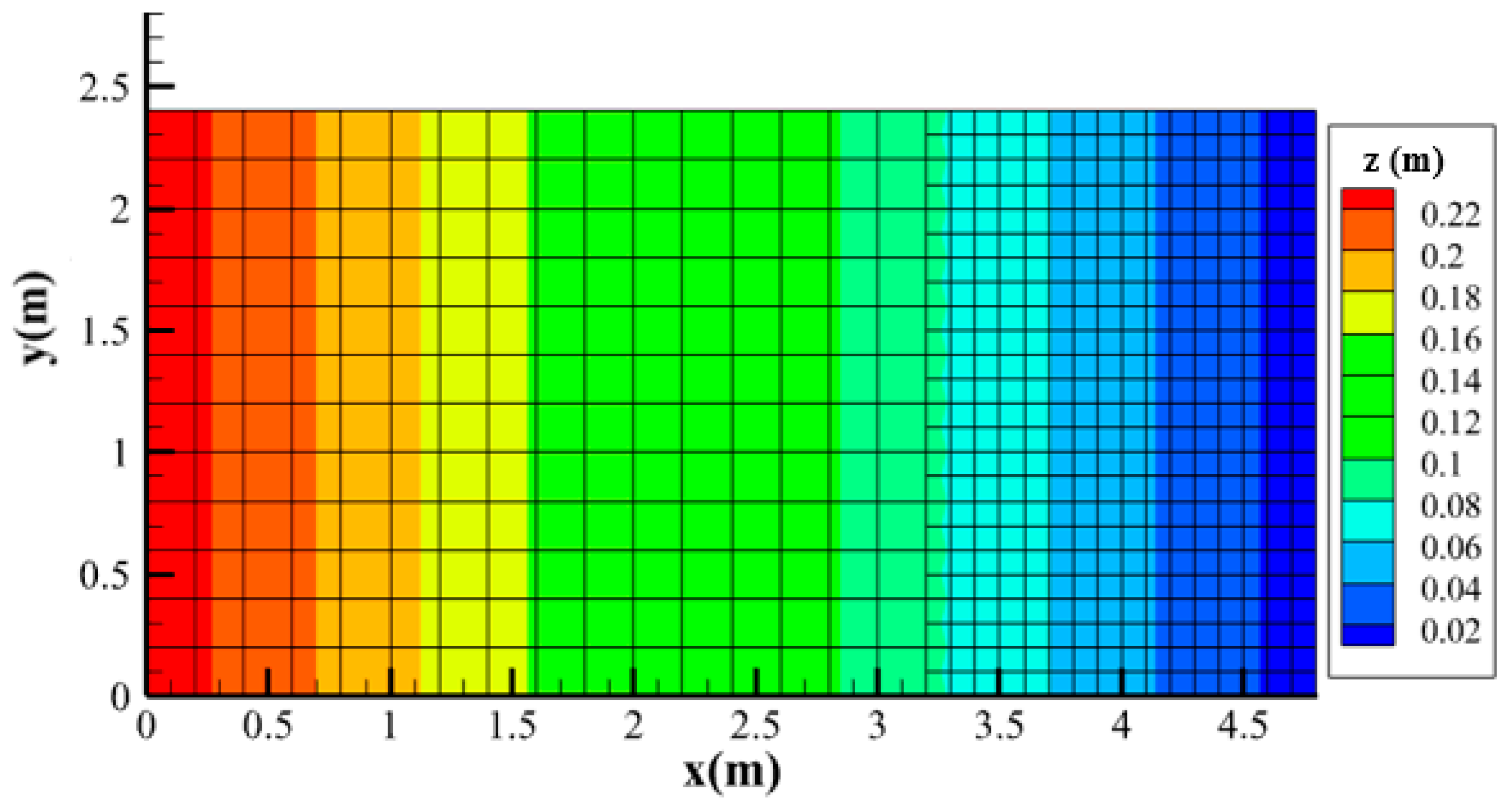
Rainfall runoff over a steep-sloped plane that has a length of 4.88 m and a width of 2.44 m was simulated based on the proposed model [28]. The characteristics of the domain used in their experiment were as follows: the bottom slope was 0.0465, and the Manning coefficient was 0.0125 s/m1/3. The rainfall intensity was 27 mm/h with a duration of 240 s, and the total simulation time was 540 s. The boundary conditions were no-flow conditions at the inlet and zero-gradient conditions at the outlet. The computational domain was divided into different grid sizes. The size of the fine grid was Δ x w = 0.1   m , while the size of the coarse grid was twice that of the fine grid. The grid partition is presented in Figure 6. The 2D hydrodynamic and DBCM models were also used to simulate the runoff under the same conditions, and the mesh space of these two models was 0.1 m.
The discharge hydrographs at the downstream boundary, as well as a comparison with the analytical solution, are shown in Figure 7. Compared with the DBCM and 2D hydrodynamic models, it was observed that the discharge hydrograph obtained from the M-DBCM was essentially identical to the analytical solution, which proved the reliability of the proposed model. The main difference between the DBCM and 2D hydrodynamic model was at peak discharge. That was mainly due to the difference between the calculation methods of these two models.
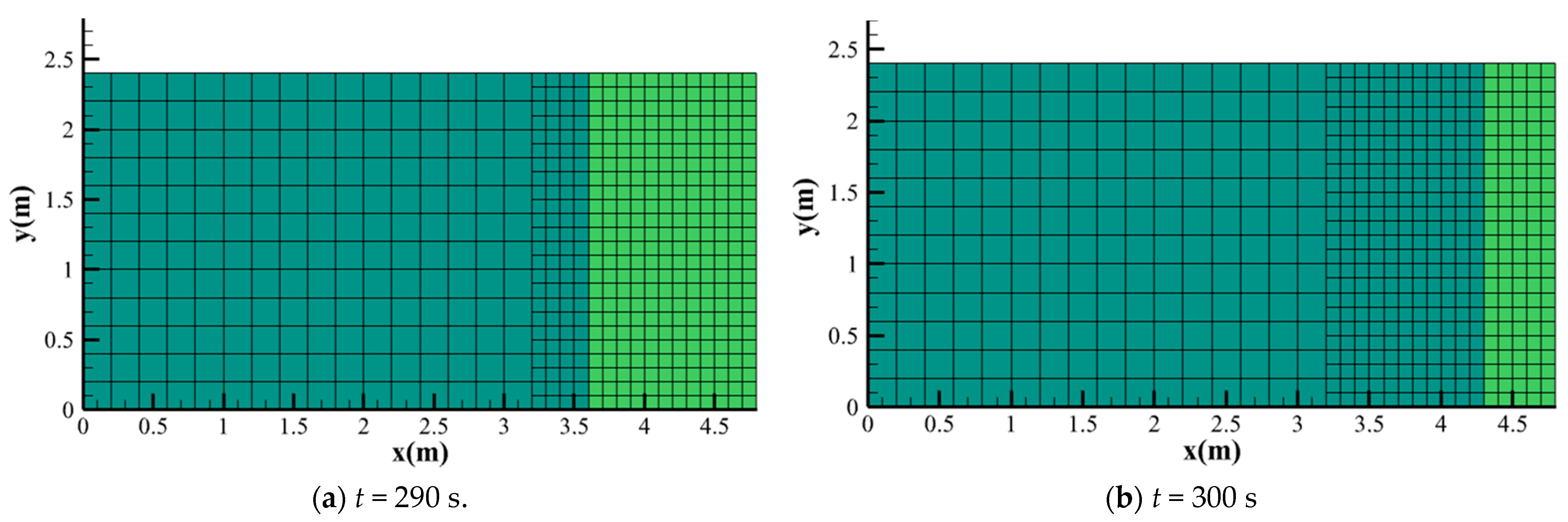
The position of the internal moving boundary between the SWEs and DWEs at different times is shown in Figure 8; the DWE zones are presented in dark green, while the SWE regions are shown in light green. Most of the regions on the fine grid were calculated using the SWEs at 290 s. From Figure 7, the discharge reached the maximum at this time, and the water depth rose in a short time. As a result, in almost all regions, the water depth was higher than the threshold, and SWEs were implemented for most of the computational domain. However, since the rainfall stopped, no extra water flowed into the domain, and therefore, the water depth was decreased. When the water depth was lower than the threshold, the DWEs were used to simulate the discharge and runoff, and the SWE regions were reduced. Therefore, at 300 s, most regions on the fine grid were considered DWE regions, and the SWE regions were reduced compared with the last moment. As a result, the coupling boundary was moved from the SWE zones to the DWE zones. The evolution of the internal moving boundary was in accordance with the natural physical process of flood formation and propagation.
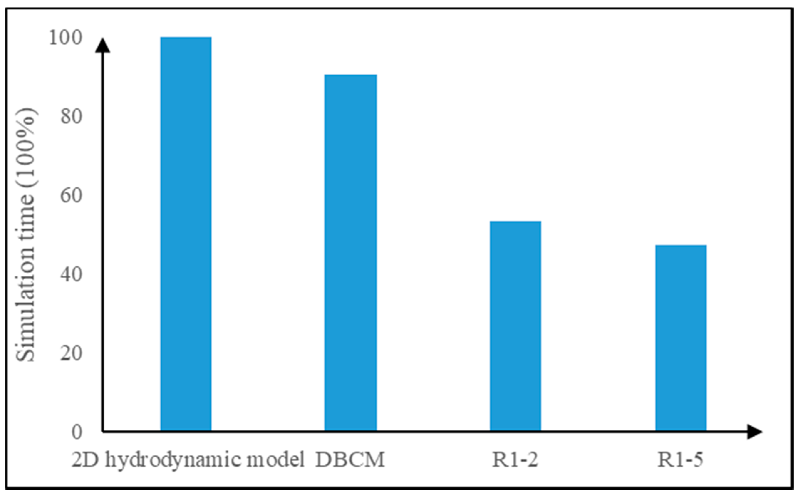
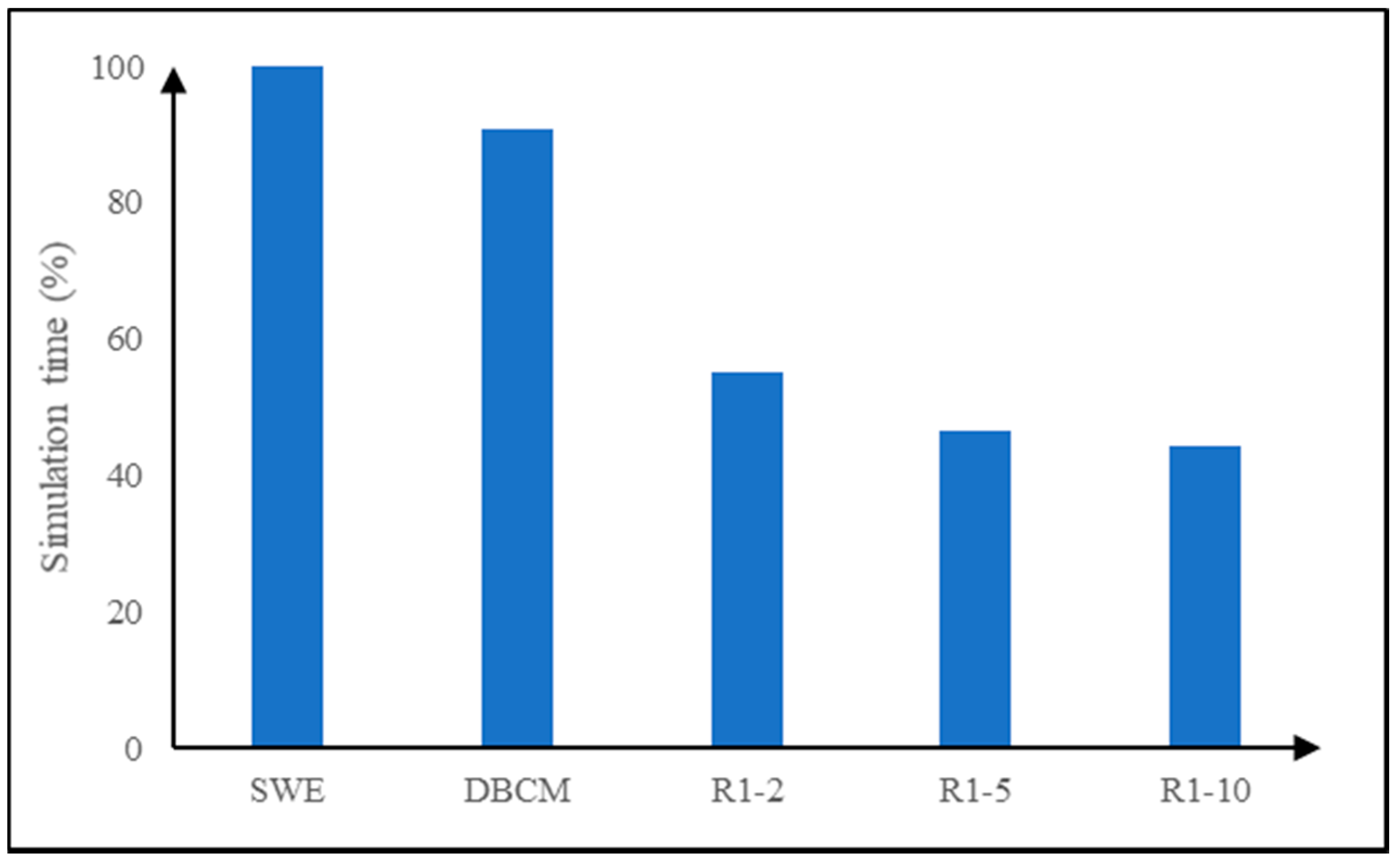
In M-DBCM, most of the regions were calculated based on the coarse grid, and only small parts of the areas where the water depth was high were simulated on the fine grid; therefore, the computational efficiency could be significantly improved compared with the DBCM or 2D hydrodynamic model. The simulation times of different models are shown in Figure 9, where “R1–2” and “R1–5” represent the size ratios of the coarse grid to the fine grid, which are 1:2 and 1:5 in the M-DBCM, respectively, and “SWE” represented the 2D hydrodynamic model. From this figure, in the 2D hydrodynamic model, since the SWEs were used to calculate the flood process in whole regions, it can take more time and have low computational efficiency, while the SWEs and DWEs can be converted to each other at different times according to the water depth threshold in the DBCM, and thus the calculation takes relatively less time. However, the computational time of the M-DBCM was reduced by half compared with the DBCM and 2D hydrodynamic model. It is well known that the computational time can be reduced if the number of calculation nodes is fewer. In this case study, there were 620 computing nodes in total, including 195 nodes on the coarse grid and 425 nodes on the fine grids in M-DBCM, where the grid size ratio was 1:2, while the number of calculation nodes was 1225 in DBCM. As a result, the computational efficiency of M-DBCM was obviously improved. In M-DBCM, as the ratio of the coarse grid and fine grid increased, the computational efficiency was also improved, which was mainly due to the reduction in the number of computing nodes in the coarse grid. Overall, it was shown that the computational efficiency was greatly improved based on the proposed M-DBCM, which can be used in practical applications.

3.3. Rainfall Runoff over a V-Shaped Watershed

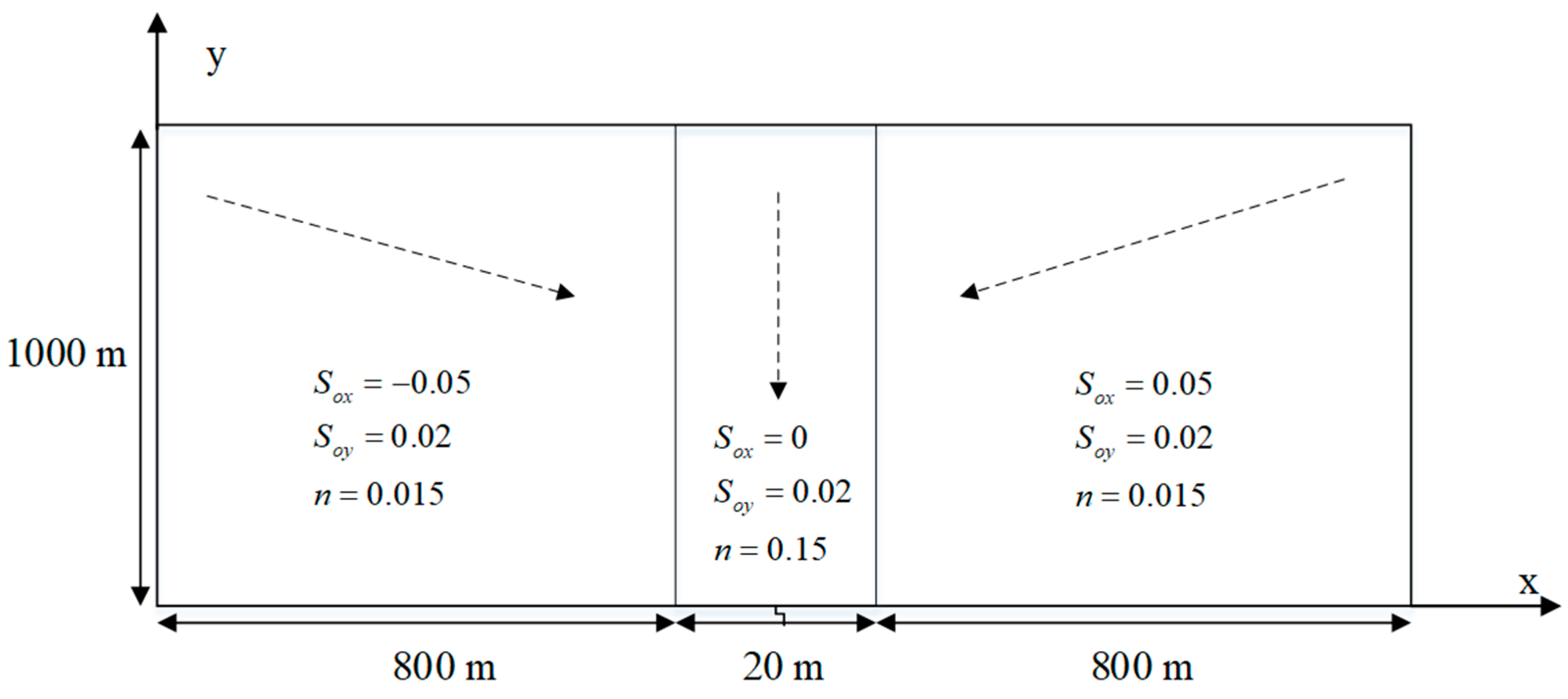
A 2D surface flow over a V-shaped catchment was simulated to verify the performance of the M-DBCM [29,33]. The computational domain was symmetrically V-shaped, with a pair of symmetrical hill slopes forming a channel at the central region. The riverbed slopes on the left and right sides were −0.05 and 0.05, respectively. The bottom slope of the channel in the x-direction was 0 but was 0.02 in the y-direction. The Manning coefficient on the hillslope was 0.015, while it was 0.15 on the main channel. The detailed dimensions and related information of the V-shaped catchment are shown in Figure 10.
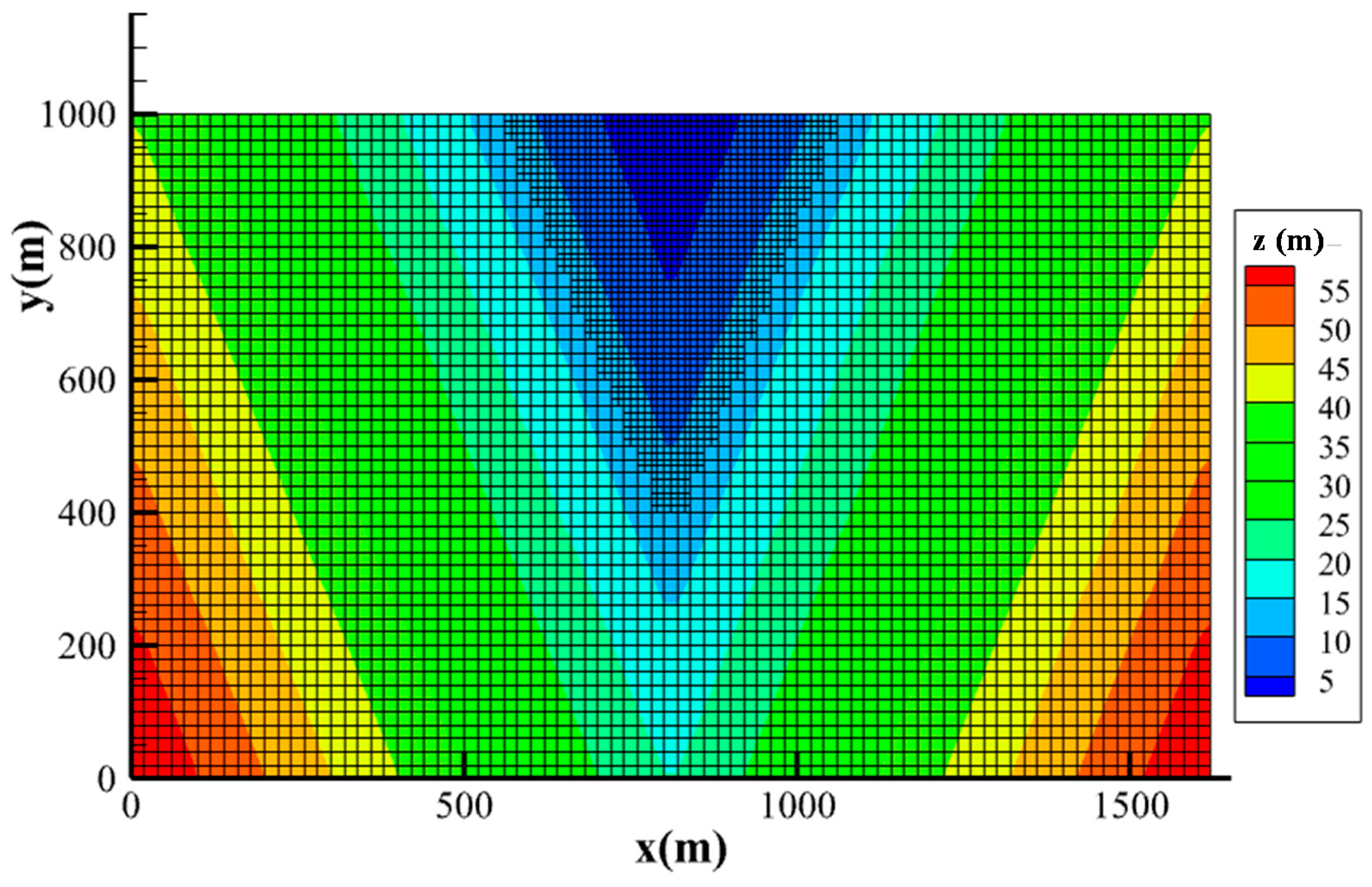
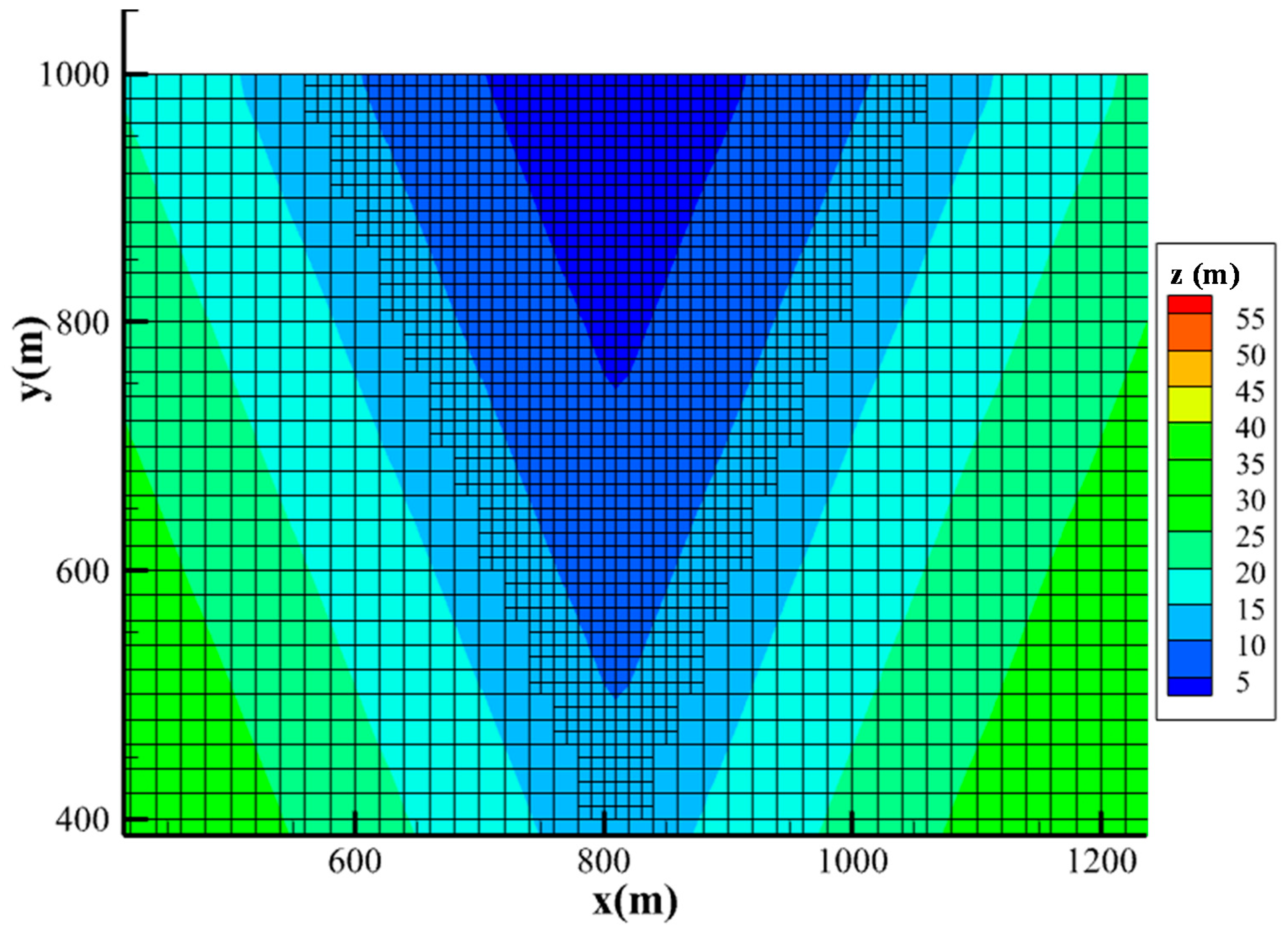
The proposed M-DBCM was used to simulate the 2D surface flow over the V-shaped domain. The total simulation time was 10,800 s, and the constant rainfall intensity was 10.8 mm/h for 5400 s. Two sizes of grid were used to divide the V-shaped catchment. The size of the coarse grid was 20 m resolution, where the DWEs were used to reduce the computational time, while the resolution of the fine grid was 10 m. The grid partition is shown in Figure 11, where a V-shaped zone near the watershed outlet was discretized using fine grids, while the others were discretized using coarse grids. To exhibit the scale of the grid size more clearly, the partition of the fine grid is amplified in Figure 12. The DBCM and 2D hydrodynamic models were also developed to verify the performance of the M-DBCM under the same conditions. In these two models, the grid size was set as Δ x = Δ y = 10   m . The results were all compared with measured data.
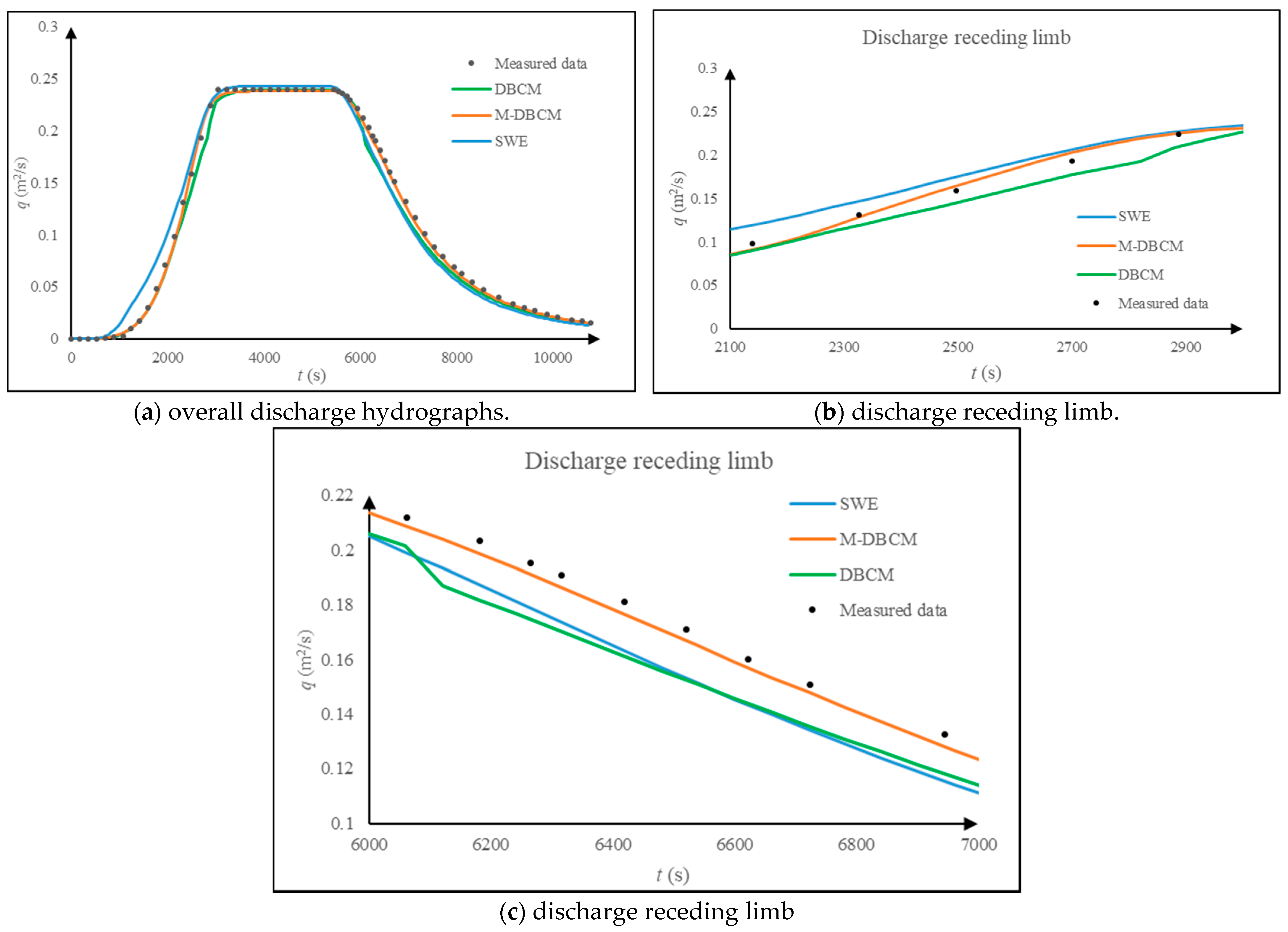
The whole discharge hydrographs obtained from different models are shown in Figure 13a, in which the “SWE” repressed the 2D hydrodynamic model, and the discharge rising limb and discharge receding limb were amplified to clearly express the differences in the hydrographs obtained from different models, as shown in Figure 13b,c. From this figure, a closer match was produced with the measured data and computed results obtained by these models, which indicated that the results were encouraging, and the overall trend was well captured. Comparing the hydrographs between the 2D hydrodynamic model and M-DBCM, the discharge hydrographs showed good agreement for the discharge receding limb and peak discharge, but for the rising limb, the hydrographs simulated by these two models were not consistent. In the rising limb, the flow calculated using DBCM and M-DBCM was lower than that simulated using the 2D hydrodynamic model. The reason for this is that the SWEs were used to calculate and simulate throughout the computational process in the 2D hydrodynamic model, while the DWEs were used to simulate the flood process when the upstream water fell below the threshold in M-DBCM and DBCM. Since there were no time partial derivative terms in the hydrologic model, the velocity at the present moment was a function of the current water level gradient, which was not equal to the velocity at the previous moment plus the flux term. However, compared with DBCM, the match of discharge hydrographs between M-DBCM and the measured data was better, which indicated that the simulation accuracy was not reduced due to the division of different grid sizes in M-DBCM.
The simulation times of the 2D hydrodynamic model, DBCM, and M-DBCM were compared, as shown in Figure 14. The 2D hydrodynamic model solved SWEs in the whole domain, while the DBCM and M-DBCM altered the SWEs and DWEs according to the water depth information. The solution of the SWEs in the whole domain needed a large volume of computational resources and time. Therefore, the DBCM and M-DBCM required less simulation time than the 2D hydrodynamic model. It can be seen from the figure that the calculation time of M-DBCM was reduced by half compared with that of DBCM. A uniform grid was adopted to divide the computing zones in DBCM, and the number of calculation nodes was about 16,463; meanwhile, most of the areas were discretized with coarse grids, and only a small part of the regions was calculated based on the fine grid in M-DBCM, and the number of calculation nodes was much lower than that in DBCM. As a result, the computational efficiency of M-DBCM was greatly improved. However, as for the M-DBCM, the computational efficiency was improved when the grid size ratio increased. The results showed that the computational efficiency was dramatically improved when different grid sizes were used to divide the computational zones, and the M-DBCM proposed in this study required less computation time without significantly compromising the simulation accuracy.
The SWE zones and DWE zones were divided according to the water depth threshold on the fine grid, and the computational domains of the SWEs and DWEs were able to switch dynamically. The location of the coupling boundary between these two algorithms at different times is shown in Figure 15, where the SWE zones are presented in yellow while the DWE regions are expressed in green. It can be clearly seen that the position of the coupling boundary was time-dependent. From Figure 15a, the water depth was high at 5400 s, when the accumulated rainfall reached the maximum, and the water depth in most areas was higher than the threshold. Therefore, most of the regions on the fine grid were defined as SWE regions. After 5400 s, when the rainfall stopped, the water depth began to decrease and became lower than the water depth threshold in most areas, leading to big DWE zones. Accordingly, from Figure 15b, the location of the coupling boundary moved to the SWE zones defined at the last moment, and the area of the SWE zones decreased. The results indicated that the coupling boundary was dynamic during the simulation, in accordance with the natural physical processes of flood formation and propagation.

3.4. M-DBCM Implemented for a Natural Watershed

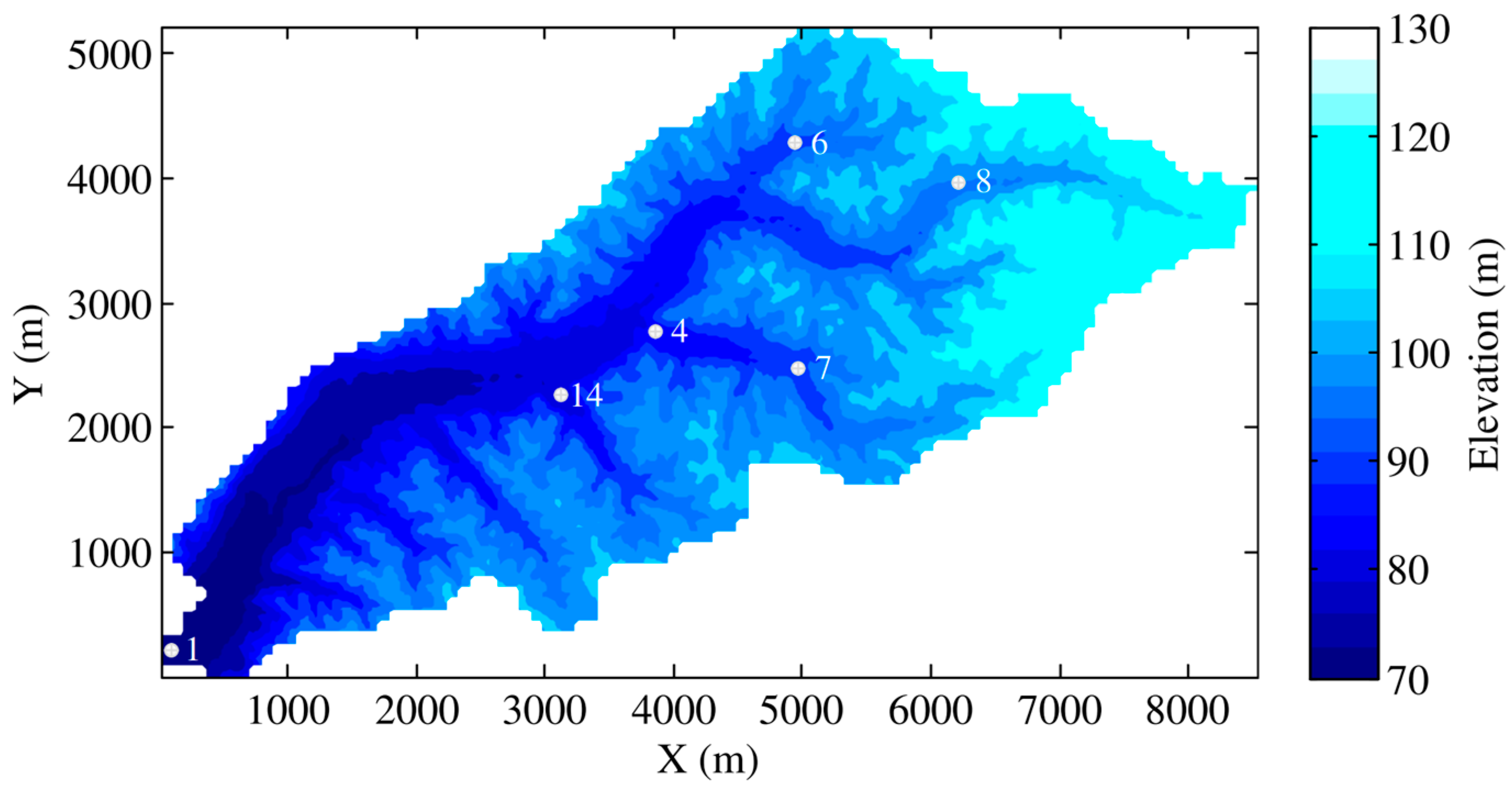
The M-DBCM was used to simulate the flood information in a natural watershed, the Goodwin Creek Experimental Watershed, in Panola County, Mississippi, USA, as shown in Figure 16. The Goodwin Creek Experimental Watershed is a tributary of Long Creek and flows into the Yocona River, Yazoo River Basin. The watershed has a catchment area of 21.3 km2, and the elevation ranges from 71–128 m. The overall terrain gradually goes down from northeast to southwest, consistent with the trend of the main channel.
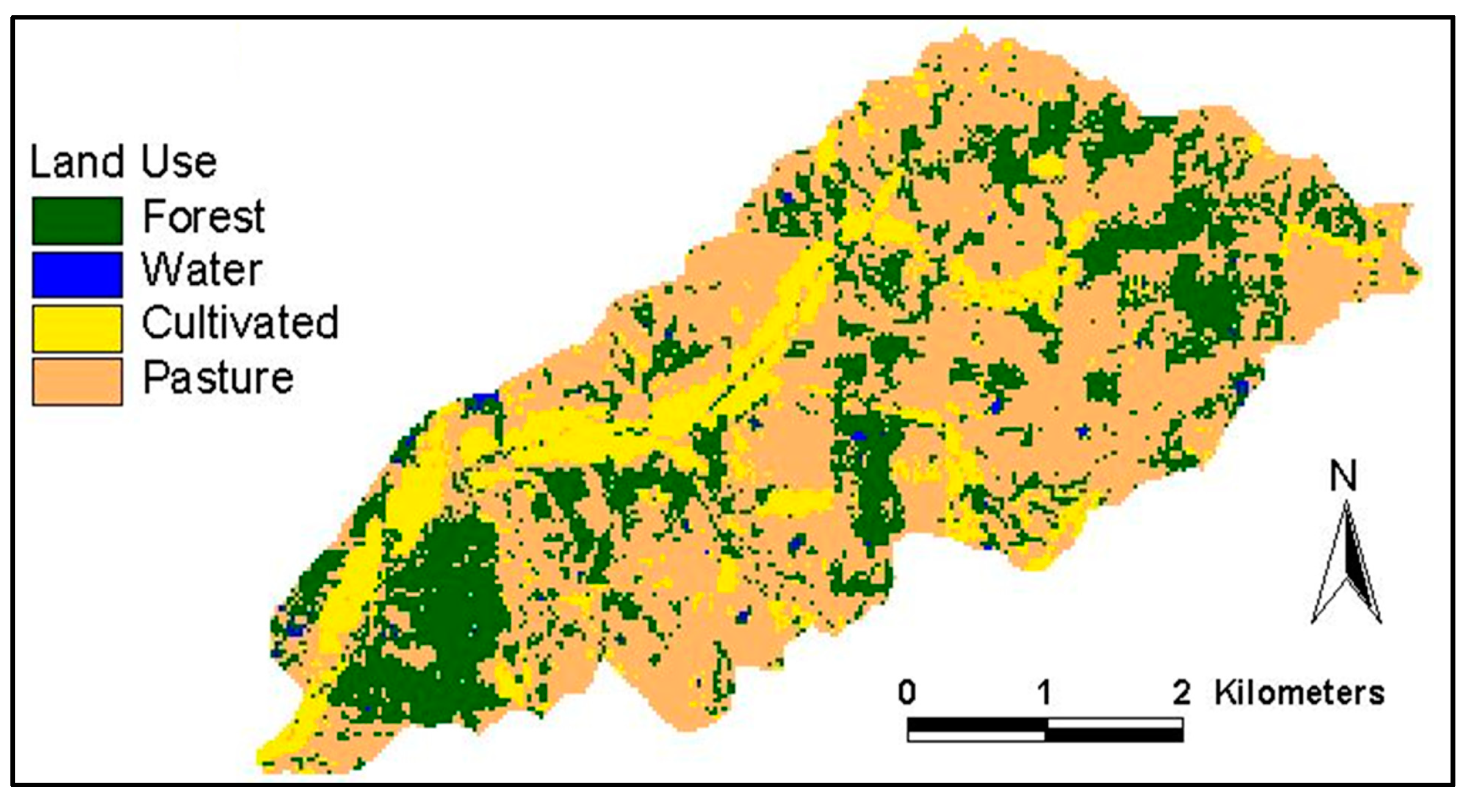
The proposed M-DBCM was applied to simulate the rainfall runoff process in the Goodwin Creek Experimental Watershed. The input datasets for M-DBCM included rainfall, DEM, land use and cover, and soil types. The rainfall event was simulated in Lai [34] and Sanchez [35] on 17 October 1981, and six stream gauges were described in the study by Sanchez [35], as shown in Figure 16. The rainfall duration was 16,200 s, and the inverse distance interpolation method was used to obtain the precipitation data over the entire watershed. The land use was divided into four classes—forest, water, cultivated, and pasture, as shown in Figure 17, and Manning’s roughness coefficients of different land use are presented in Table 1. In addition, seven soil types were identified in the watershed, as shown in Figure 18, and the infiltration coefficients of each soil type are described in Table 2. The soil type, land use, precipitation, and DEM data were also obtained from the studies of Sanchez [35] and Blackmarr [36].
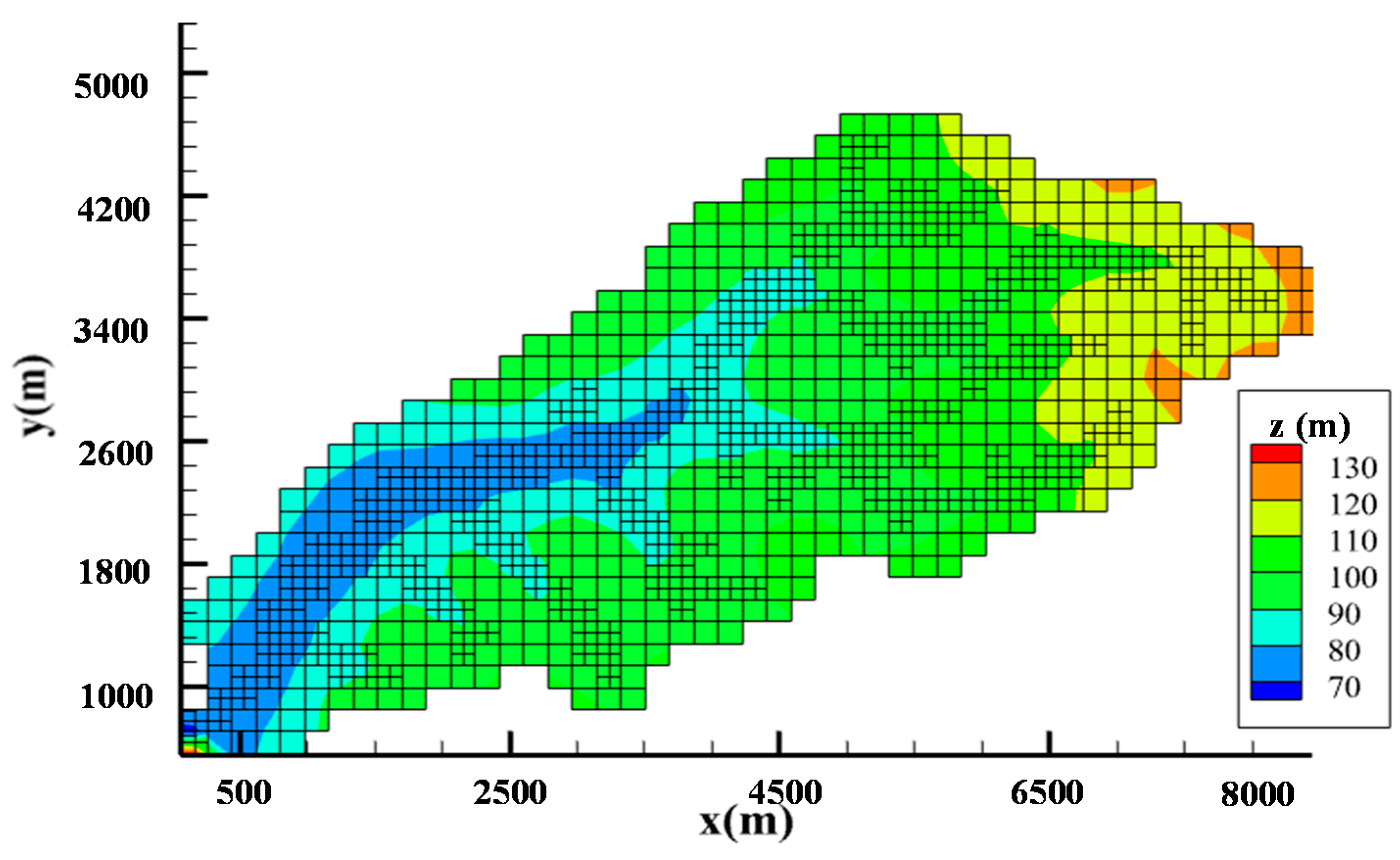
Based on a rectangular grid, the Goodwin Creek Experimental Watershed was divided into zones with different grid sizes to facilitate the setup of the M-DBCM. The DWE calculation was performed on a coarse grid at 180 m resolution to reduce the computational cost, while the spatial step size was Δ x w = Δ y w = 90   m for the fine grid to detail the flood inundation extent. The division of the computational domain is shown in Figure 19. In Figure 19, since the main channel was vulnerable to flooding, it was discretized by a fine grid, and the others were calculated based on the coarse grid. This increased the computing efficiency and decreased its complexity. The time step was dynamically adjusted according to the CFL conditions, and the total simulation time was 42,000 s. The simulation results obtained from the 2D hydrodynamic model under the same conditions were used to validate the performance of the M-DBCM. The mesh spacing was 90 m, and the number of the cells was 9310. All the results were compared with the measured data.
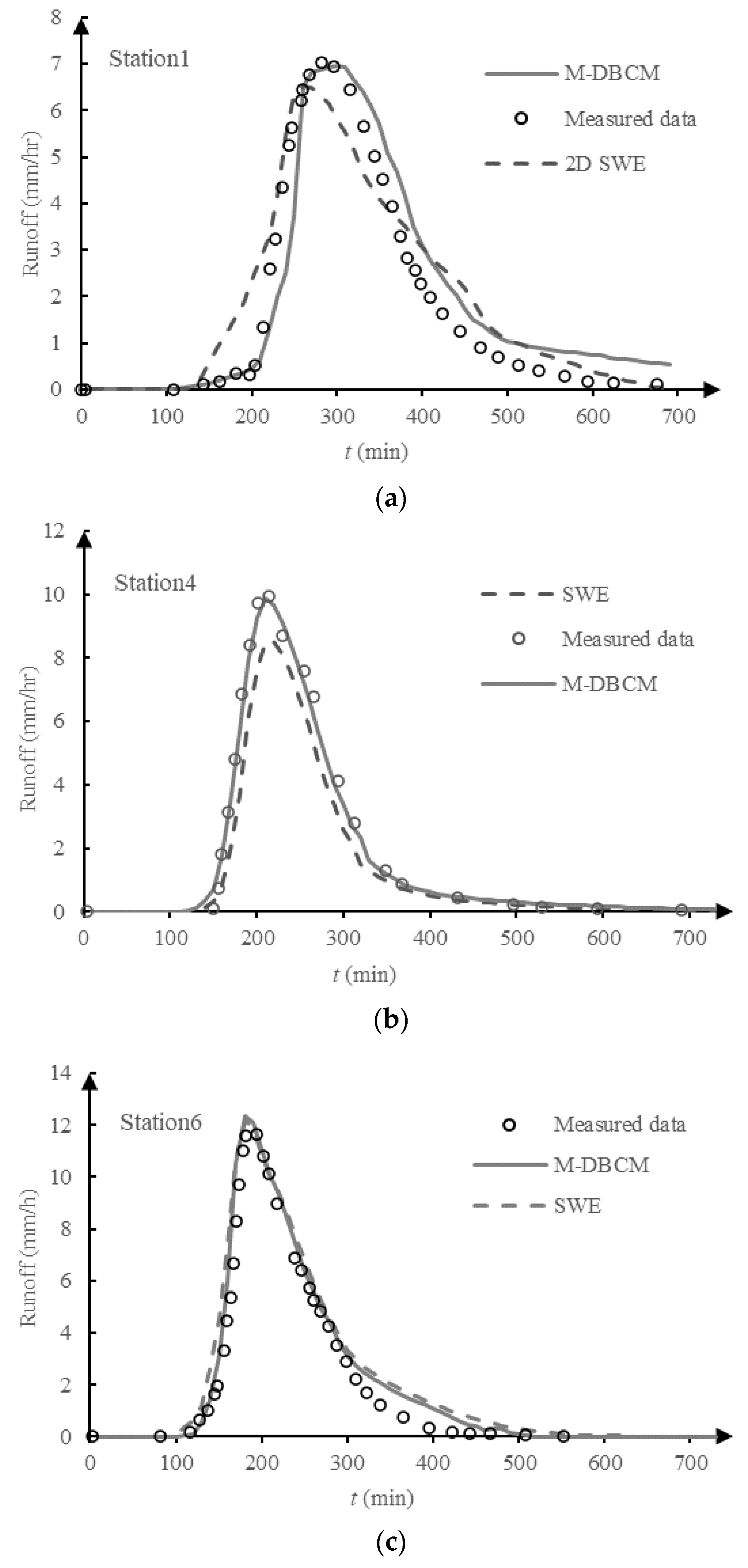
The measured data and simulated discharge hydrographs at the six gauges are compared in Figure 20. The hydrographs from the M-DBCM and 2D hydrodynamic model matched the peak arriving times, and the peak discharges very well, except for a few stations, which showed the rationality of the M-DBCM proposed in this study. For Station 1, it was found that the hydrograph obtained from the 2D hydrodynamic model was well off the measured data in comparison with the M-DBCM. The discharge hydrographs simulated by M-DBCM were not exactly consistent with the measured data in the receding limb. Several reasons may explain this phenomenon. In the simulation process, the accuracy of the input data, such as the topography, infiltration rate, roughness, and so on, can influence the results. There was also uncertainty in the observation data. This problem may be solved by sensitivity analysis in future research. In addition, it was noted that a significant overprediction of the peak occurred for Station 8. Station 8 was located in the small sub-watershed; therefore, errors may be attributed to sources such as the accuracy of precipitation and the difference in mesh size and density for the sub-watershed. Furthermore, the results of the M-DBCM and 2D hydrodynamic models were close but not exactly the same. This may be attributed to a slight difference in the calculation method between the two models. The SWEs were used in all areas in the 2D hydrodynamic model, while the M-DBCM switched between SWEs and DWEs according to the water depth. The algorithm using the SWEs in shallow waters had numerical instability [28], which could reduce the accuracy. Additionally, the uniform grid was used to divide the computational domain in the 2D hydrodynamic model, and the SWEs were implemented in whole regions, which inevitably increased the calculation time. In this case, it took about 77 s to simulate the rainfall runoff with M-DBDM, while the 2D hydrodynamic model took 135 s, indicating that the computational efficiency of M-DBCM was significantly higher than that of the 2D hydrodynamic model. On the one hand, the number of calculation nodes and cells of the 2D hydrodynamic model was far more than that of M-DBCM, which can increase the computing time. Additionally, the SWEs were solved in the whole computational domain, which not only cost a lot of time but was also prone to instability in regions with shallow water. Overall, the results showed that the M-DBCM proposed in this study can improve computational efficiency while maintaining calculation accuracy.
To quantify the error of each model, the root mean square error (RMSE) was used in this study. The RMSE is used to measure the deviation between the observed value and the true value. A smaller RMSE indicates higher accuracy. If the RMSE is 0, the observed value is equal to the true value. If the RMSE is less than half of the standard deviation of the observed value, it indicates that the performance of the model is good. The calculation of the RMSE was as follows:
RMSE = n = 1 N ( S n M n ) 2 N
where N was the number of the sample points; S n was the simulation value, and M n was the measured data.
The RMSE values of M-DBCM and the full 2D hydrodynamic model are given in Table 3, compared with the CASC2D and the model proposed by Yu and Duan [6]. The CASC2D is a typical model that was used to simulate discharge hydrographs by employing different numerical solvers for overland and channel flow and the simulation of runoff in the Goodwin Creek watershed using CASC2D was shown in [34]. From Table 3, the RMSE of M-DBCM and SWEs were lower than for CASC2D and the model proposed by Yu and Duan [6], which indicated that the model proposed in this study performs well. The RMSE of M-DBCM was closer to the SWEs but slightly lower than the RMSE of SWEs, which showed that the M-DBCM has good accuracy. Compared with others, the developed M-DBCM can simulate the rainfall runoff more accurately and efficiently, which provides a new tool for flood simulation in watersheds.
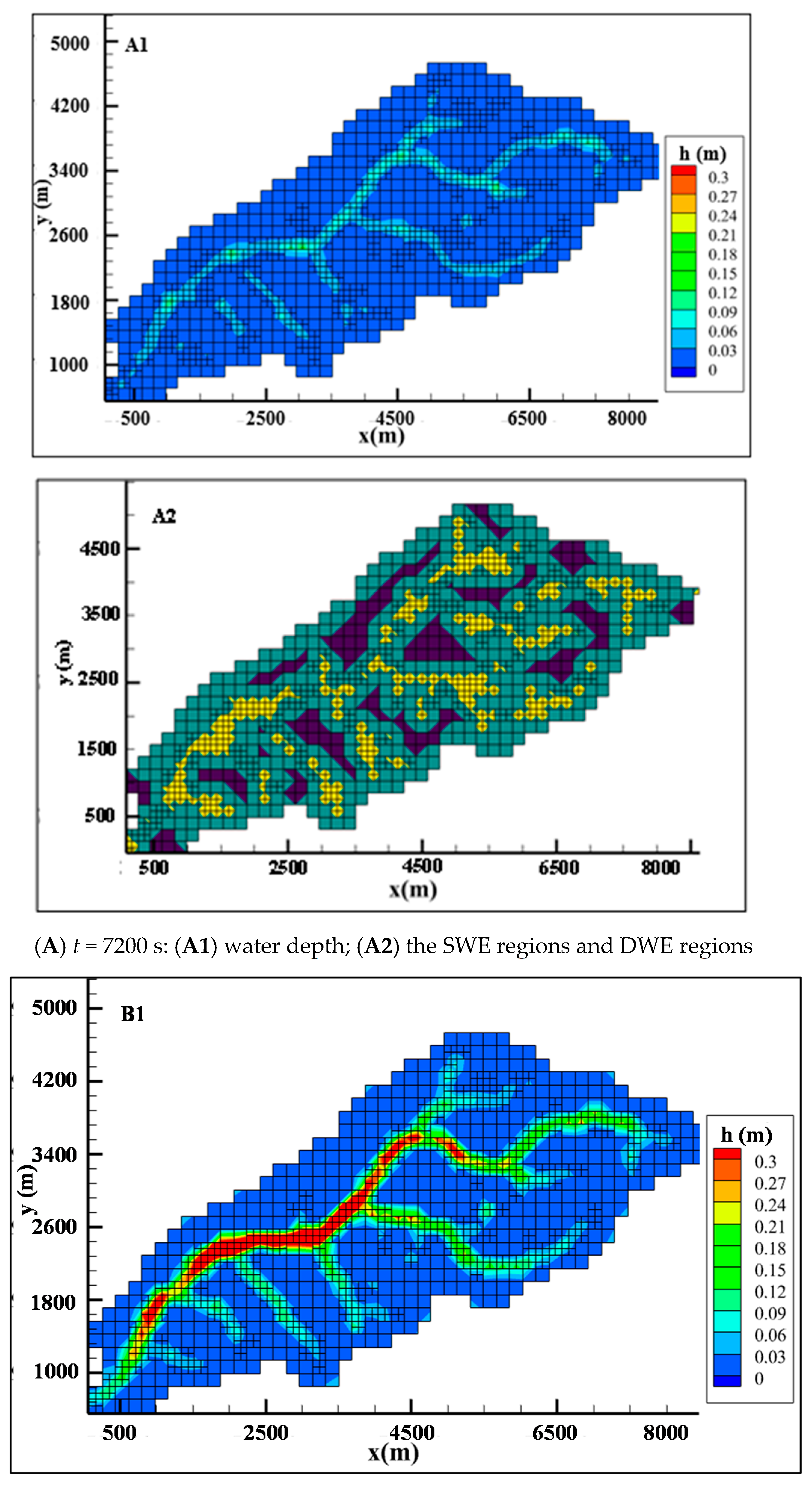
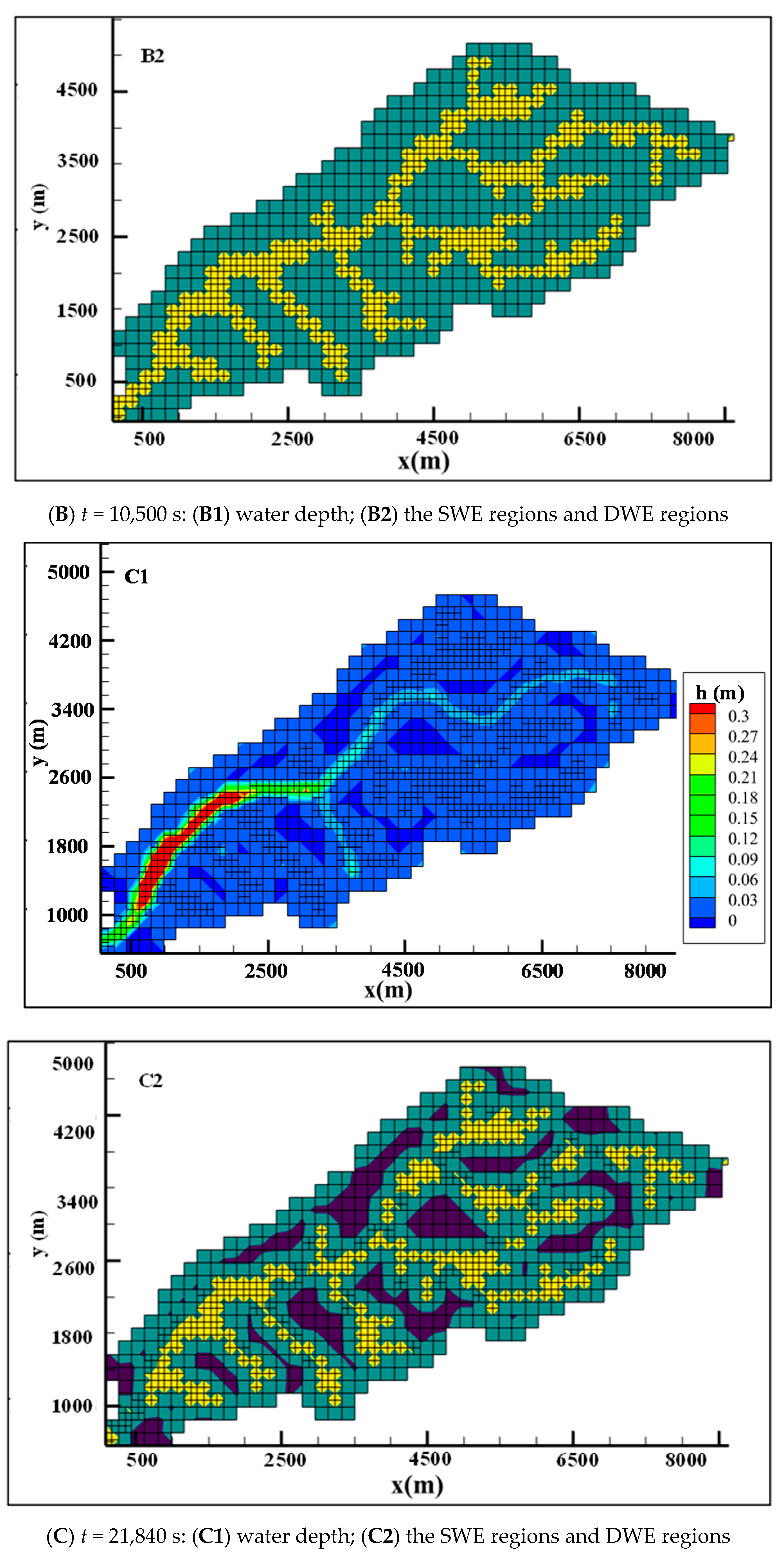
Water depth and the position of the coupling boundary at different times are presented in Figure 21. In Figure 21(A2,B2,C2), the SWE regions are marked by yellow while the DWE regions are marked by green. The black in Figure 21(A2,C2) indicates that the regions could not be calculated; that is, the water depth was approximately 0.
From Figure 21(A1), at 7200 s, the flow had not reached the peak yet at the beginning of the rainfall. The water depth in most areas of the Goodwin Creek Watershed was shallow, except for some parts of the main channel. Since the computational domain was discretized based on water depth, from Figure 21(A2), a few regions in the river were considered SWE zones, while the rest were defined as DWE zones.
The peak discharge increased gradually with the development of the rainfall at 10,500 s, and the water depth in the computational domain increased in a short period of time. At this time, since the water depth in most of the regions was higher than the water depth threshold on the fine grid, the SWEs were used to simulate flood inundation in most of the regions on the fine grid. Therefore, the SWE zones were further expanded, and thus the position of the coupling boundary was also changed, as shown in Figure 21(B2).
When the rainfall stopped, the peak discharge was decreased, so the water depth also decreased, as shown in Figure 21(C1). Once the water depth was lower than the threshold, the DWEs were used to simulate the runoff. Therefore, from Figure 21(C2), it can be seen that most regions were considered as DWE regions, and only a small part of the river channel was defined as a SWE region. Compared with the last moment, the DWE zones were extended, while the SWE regions were reduced since the coupling boundary was moved to the SWE zones.

4. Discussion

In this study, three different cases were simulated to verify the performance of the proposed model. The 2D full hydrodynamic model and DBCM were also used to simulate the runoff under the same conditions to verify the performance of the M-DBCM. Compared with others, the hydrographs simulated using M-DBCM matched the analytical solution better, which proved that the proposed method converged to the analytical solutions. The simulation results obtained from the DBCM were closer to the analytical solution than that of the 2D hydrodynamic model. The SWEs were solved in the whole computational domain and had numerical instability when the water depth was shallow, while the DBCM and M-DBCM could switch the SWEs to DWEs when the water depth was shallow; therefore, the simulation accuracy of the 2D hydrodynamic model was lower than that of M-DBCM and DBCM.
It is well known that computational time can be saved if the number of calculation nodes is low. In M-DBCM, most regions were calculated based on the coarse grid, and only a small part of areas where the water depth was high was simulated on the fine grid. Therefore, the calculation nodes of M-DBCM were fewer than those of DBCM or the 2D hydrodynamic model, and the computational efficiency was significantly improved compared with that of DBCM or the 2D hydrodynamic model. The simulation times for different models in these three cases were compared. The results showed that M-DBCM can save computational costs while maintaining good accuracy.
The runoff in the Goodwin Creek Experimental Watershed was simulated using the M-DBCM, and the hydrograph was compared with the full 2D hydrodynamic model. The results showed that the hydrographs from the M-DBCM and 2D hydrodynamic model matched the peak arriving times and the peak discharges very well, except for a few stations, which showed the rationality of the M-DBCM proposed in this study. The RMSE of solutions obtained by M-DBCM and the 2D full hydrodynamic model was compared with the CASC2D and the model proposed by Yu and Duan [6]. The RMSE of M-DBCM was lower than for the others, indicating that the M-DBCM has high calculation accuracy. In this case, it took about 77 s to simulate the rainfall runoff with M-DBDM, while the 2D hydrodynamic model took 135 s, which indicated that the computational efficiency of M-DBCM was significantly higher than that of the 2D hydrodynamic model. Overall, the results showed that the M-DBCM proposed in this study can improve the computational efficiency while maintaining the calculation accuracy, which could provide a foundation for flood disaster prevention and control.

5. Conclusions

The surface flow routing was simulated by the coupling hydrologic model and hydrodynamic model, combining the advantages of the simple calculation of the hydrologic model and high prediction accuracy of the hydrodynamic model. Various coupling models of hydrology and hydrodynamics for flood prediction in watersheds were compared in this paper. The external coupling was in one-way sequential coupling models, which had the advantages of simple development, but the accuracy of the one-way coupling was relatively low. The full 2D dynamic flood model had the advantage of high accuracy, but it took more computational time than the external coupling models. The hydrologic model and 1D hydrodynamic model were coupled in a dynamic bidirectional manner, which reflected the mutual interactions between the hydrologic and 1D hydrodynamic processes. The indirect dynamic bidirectional coupling between the distributed hydrologic model and the 2D hydrodynamic model required a connection channel through a 1D hydrodynamic model. The DBCM was a direct dynamic bidirectional coupling between the SWEs and DWEs, which was proposed by the author’s group in 2021 [29]. The DWEs were connected to the SWEs through a coupling moving boundary, and the DBCM could reflect the interaction between the hydrological process and the hydrodynamic process, which ensured the conservation of mass and momentum through coupling the dynamic boundary. In DBCM, the SWEs were solved explicitly only in the local region, which enabled good computational efficiency and numerical stability.
Although the computational efficiency and numerical stability can be optimized to a certain extent in the DBCM, the computational efficiency can be further improved. In this study, a dynamic bidirectional coupling of SWEs and DWEs based on different grid sizes was proposed to simulate the surface flow routing. The computational domain was discretized according to the watershed terrain elevation, where the regions that were prone to floods were divided into a fine grid, while the others were divided into a coarse grid. The DWEs were used in thin-layer water regions with a larger-scale grid to reduce the computational costs and improve the numerical stability, while in the areas with a small grid size, the DWEs and SWEs were switched according to water depth to detail the inundation evolution, such as water depth, inundation duration, and so on. In fine grid zones, the DWEs and SWEs were coupled based on an internal moving boundary, and there was a mutual interaction between these two algorithms. The conservation of mass and momentum on the internal moving boundary was guaranteed by using the CCFV scheme, which improved the accuracy of the proposed model. Three case studies were used to prove the performance of the proposed M-DBCM. The results revealed that the M-DBCM had good computational efficiency while maintaining satisfactory simulation accuracy. A flood in the Goodwin Creek Watershed was simulated and calculated. The results obtained from M-DBCM matched well with the measured data, and the water depth was changed with the rainfall, and thus the coupling boundary was also changed. Compared with the full 2D hydrodynamic model, the M-DBCM had high computational efficiency and good numerical stability while maintaining calculation accuracy.
However, the M-DBCM is a newly proposed model, which will have a broader application prospect after improvement. For example, the groundwater simulation could be developed, and the exchanges between surface and groundwater flows considered. Parameter sensitivity analysis could be included to prove the performance of the proposed model. In future research, the 1D river hydrodynamic model and urban drainage network model needs to be added; this research work is in progress.

Author Contributions

Conceptualization, C.J. and Q.Z.; methodology, Y.S.; software, Q.Z.; validation, Y.S.; formal analysis, Y.S.; investigation, C.J.; resources, C.J.; data curation, Q.Z.; writing—original draft preparation, Y.S.; writing—review and editing, D.Z. (Dejun Zhu); visualization, D.Z. (Di Zhang); supervision, C.J.; project administration, C.J.; funding acquisition, C.J. and D.Z. (Dejun Zhu). All authors have read and agreed to the published version of the manuscript.

Funding

This research was co-funded by the National Science Foundation of China [No. 52179068, 52179069], and the Key Laboratory of Hydroscience and Engineering, grant number [No. 2021-KY-04].

Institutional Review Board Statement

Not applicable.

Informed Consent Statement

Written informed consent has been obtained from the patient(s) to publish this paper.

Data Availability Statement

Not applicable.

Acknowledgments

The authors thank the anonymous reviewers for their valuable comments.

Conflicts of Interest

The authors declare no conflict of interest.

References

  1. Tomasz, D.; Ewelina, S.; Joanna, W.D. Long-term impact of sediment deposition and erosion on water surface profiles in the Ner River. Water 2017, 9, 168–182. [Google Scholar]
  2. Hua, J.; Rui, L.; Yu, W.; Prasad, T. Flood-runoff in semi-arid and sub-humid regions, a case study: A simulation of Jianghe watershed in northern china. Water 2015, 7, 5155–5172. [Google Scholar]
  3. Leandro, J.; Chen, A.S.; Schumann, A. A 2D parallel diffusive wave model for floodplain inundation with variable time step (P-DWave). J. Hydrol. 2014, 517, 250–259. [Google Scholar] [CrossRef]
  4. Eum, H.-I.; Dibike, Y.; Prowse, T. Climate-induced alteration of hydrologic indicators in the athabasca river basin, alberta, canada. J. Hydrol. 2016, 544, 327–342. [Google Scholar] [CrossRef]
  5. Yang, W.; Long, D.; Bai, P. Impacts of future land cover and climate changes on runoff in the mostly afforested river basin in north china. J. Hydrol. 2019, 570, 201–219. [Google Scholar] [CrossRef]
  6. Yu, C.; Duan, J. Two-dimensional hydrodynamic model for surface-flow routing. J. Hydraul. Eng. 2014, 140, 04014045. [Google Scholar] [CrossRef]
  7. Mishra, B.K.; Emam, A.R.; Masago, Y.; Kumar, P.; Regmi, R.K.; Fukushi, K. Assessment of future flood inundations under climate and land use change scenarios in the ciliwung river basin, jakarta. J. Flood Risk Manag. 2018, 11, S1105–S1115. [Google Scholar] [CrossRef]
  8. Liu, Z.J.; Hashim, N.B.; Kingery, W.L.; Huddleston, D.H.; Xia, M. Hydrodynamic modeling of St. Louis Bay estuary and watershed using EFDC and HSPF. J. Coast. Res. 2008, 52, 107–116. [Google Scholar] [CrossRef]
  9. Li, W.; Lin, K.; Zhao, T.; Lan, T.; Chen, X.; Du, H.; Chen, H. Risk assessment and sensitivity analysis of flash floods in ungauged basins using coupled hydrologic and hydrodynamic models. J. Hydrol. 2019, 572, 108–120. [Google Scholar] [CrossRef]
  10. Dargahi, B.; Setegn, S.G. Combined 3D hydrodynamic and watershed modeling of Lake Tana, Ethiopia. J. Hydrol. 2011, 398, 44–64. [Google Scholar] [CrossRef]
  11. Bravo, J.M.; Allasia, D.; Paz, A.R.; Collischonn, W.; Tucci, C.E.M. Coupled Hydrologic-Hydraulic Modeling of the Upper Paraguay River Basin. J. Hydrol. Eng. 2012, 17, 635–646. [Google Scholar] [CrossRef]
  12. Laganier, O.; Ayral, P.A.; Salze, D.; Sauvagnargues, S. A coupling of hydrologic and hydraulic models appropriate for the fast floods of the gardon river basin (France). Nat. Hazards Earth Syst. Sci. 2014, 14, 2899–2920. [Google Scholar] [CrossRef] [Green Version]
  13. Hdeib, R.; Abdallah, C.; Colin, F.; Brocca, L.; Moussa, R. Constraining coupled hydrological-hydraulic flood model by past storm events and post-event measurements in data-sparse regions. J. Hydrol. 2018, 540, 160–176. [Google Scholar] [CrossRef]
  14. Choi, C.C.; Mantilla, R. Development and analysis of GIS tools for the automatic implementation of 1D hydraulic models coupled with distributed hydrological models. J. Hydrol. Eng. 2015, 20, 06015005. [Google Scholar] [CrossRef]
  15. Gomes, M.M.D.; Verçosa, L.F.D.; Cirilo, J.A. Hydrologic models coupled with 2D hydrodynamic model for high-resolution urban flood simulation. Nat. Hazards 2021, 108, 3121–3157. [Google Scholar] [CrossRef]
  16. Bhola, P.K.; Leandro, J.; Disse, M. Framework for offline flood inundation forecasts for two-dimensional hydrodynamic models. Geosciences 2018, 8, 346. [Google Scholar] [CrossRef] [Green Version]
  17. Liu, Z.; Zhang, H.; Liang, Q. A coupled hydrological and hydrodynamic model for flood simulation. Hydrol. Res. 2019, 50, 580–606. [Google Scholar] [CrossRef]
  18. Thompson, J.R.; Sørenson, H.R.; Gavin, H.; Refsgaard, A. Application of the coupled MIKE SHE/MIKE 11 modelling system to a lowland wet grassland in southeast England. J. Hydrol. 2004, 590, 151–179. [Google Scholar] [CrossRef]
  19. Chalkidis, I.; Seferlis, M.; Sakellariou-Makrantonaki, M. Evaluation of the environmental impact of an irrigation network in a ramsar area of the greek part of the strymonas river basin using a coupled Mike SHE/Mike 11 modelling system. Glob. Nest J. 2016, 18, 56–66. [Google Scholar]
  20. Laganier, O.; Ayral, P.A.; Salze, D.; Sauvagnargues, S. A coupling of hydrologic and hydraulic models appropriate for the fast floods of the Gardon river basin (France): Results and comparisons with others modelling options. Nat. Hazards Earth Syst. Sci. 2013, 1, 4635–4680. [Google Scholar] [CrossRef] [Green Version]
  21. Chen, W.; Huang, G.; Han, Z. Urban stormwater inundation simulation based on SWMM and diffusive overland-flow model. Water Sci. Technol. 2017, 76, 3392–3403. [Google Scholar] [CrossRef]
  22. Chen, W.; Huang, G.; Han, Z.; Wang, W. Urban inundation response to rainstorm patterns with a coupled hydrodynamic model: A case study in Haidian Island, China. J. Hydrol. 2018, 564, 1022–1035. [Google Scholar] [CrossRef]
  23. Seyoum, S.D.; Vojinovic, Z.; Price, R.K.; Weesakul, S. Coupled 1D and noninertia 2D flood inundation model for simulation of urban flooding. J. Hydraul. Eng. 2012, 138, 23–34. [Google Scholar] [CrossRef]
  24. Wu, J.; Yang, R.; Song, J. Effectiveness of low-impact development for urban inundation risk mitigation under different scenarios: A case study in Shenzhen, China. Nat. Hazards Earth Syst. Sci. 2018, 18, 2525–2536. [Google Scholar] [CrossRef] [Green Version]
  25. Brewer, S.K.; Worthington, T.A.; Mollenhauer, R.; Stewart, D.R.; Mcmanamay, R.A.; Guertault, L.; Moore, D. Synthesizing models useful for ecohydrology and ecohydraulic approaches: An emphasis on integrating models to address complex research questions. Ecohydrology 2018, 11, e1966. [Google Scholar] [CrossRef]
  26. Hou, J.; Liang, Q.; Simons, F.; Hinkelmann, R. A 2D well balanced shallow flow model for unstructured grids with novel slope source term treatment. Adv. Water Resour. 2013, 52, 107–131. [Google Scholar] [CrossRef]
  27. Yu, C.; Duan, J.G. Simulation of surface runoff using hydrodynamic model. J. Hydrol. Eng. 2017, 22, 04017006. [Google Scholar] [CrossRef]
  28. Kim, J.; Warnock, A.; Ivanov, V.Y.; Katopodes, N.D. Coupled modeling of hydrologic and hydrodynamic processes including overland and channel flow. Adv. Water Resour. 2012, 37, 104–126. [Google Scholar] [CrossRef]
  29. Jiang, C.; Zhou, Q.; Yu, W.; Yang, C.; Lin, B. A dynamic bidirectional coupled surface flow model for flood inundation simulation. Nat. Hazards Earth Syst. Sci. 2021, 21, 497–515. [Google Scholar] [CrossRef]
  30. Liang, Q. Flood simulation using a well-balanced shallow flow model. J. Hydraul. Eng. 2010, 136, 669–675. [Google Scholar] [CrossRef]
  31. Leer, B.V. Towards the ultimate conservative difference scheme V: A second order sequel to Godunov′s method. J. Comput. Phys. 1979, 32, 101–136. [Google Scholar] [CrossRef]
  32. Delis, A.; Nikolos, I. A novel multidimensional solution reconstruction and edge-based limiting procedure for unstructured cell-centered finite volumes with application to shallow water dynamics. Int. J. Numer. Methods Fluids 2013, 71, 584–633. [Google Scholar] [CrossRef]
  33. Panday, S.; Huyakorn, P.S. A fully coupled physically-based spatially-distributed model for evaluating surface/subsurface flow. Adv. Water Resour. 2004, 27, 361–382. [Google Scholar] [CrossRef]
  34. Lai, Y.G. Watershed runoff and erosion modeling with a hybrid mesh model. J. Hydrol. Eng. 2009, 14, 15–26. [Google Scholar] [CrossRef]
  35. Sánchez, R.R. GIS-Based Upland Erosion Modeling, Geovisualization and Grid Size Effects on Erosion Simulations with CASC2D-SED. Ph.D. Thesis, Colorado State University, Fort Collins, CO, USA, June 2002. [Google Scholar]
  36. Blackmarr, W. Documentation of Hydrologic, Geomorphic, and Sediment Transport Measurements on the Goodwin Creek Experimental Watershed, Northern Mississippi, for the Period 1982—1993; Technical Report for United States Department of Agriculture: Oxford, MS, USA, October 1995. [Google Scholar]
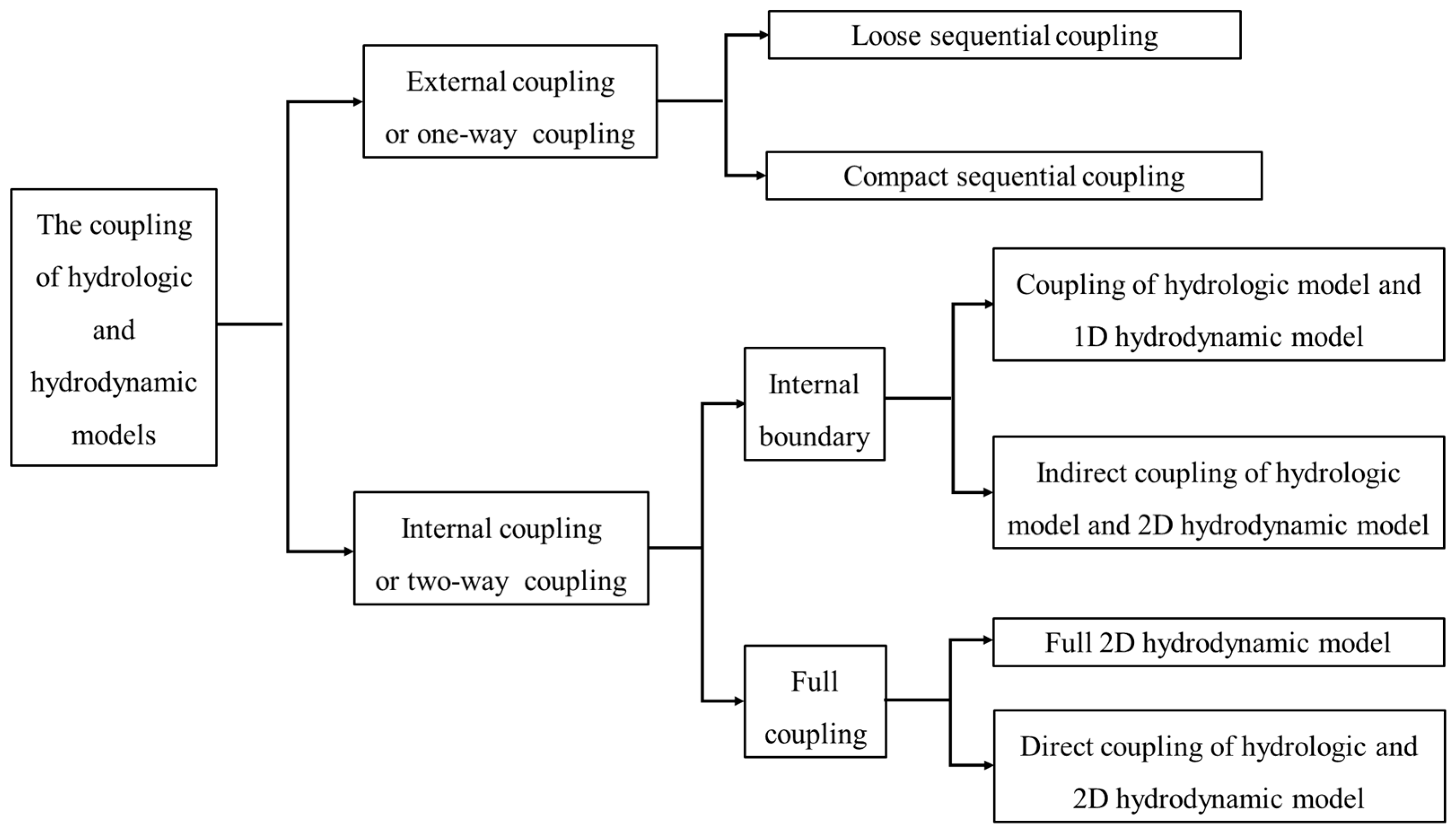
Figure 1. The classification of the coupling of the hydrologic and hydrodynamic models.
Water 13 03454 g001
Figure 2. Schematic diagram of zone partition.
Water 13 03454 g002
Figure 3. The variable interpolations between the coarse and fine grids.
Water 13 03454 g003
Figure 4. The coupling process between SWEs and DWEs based on different grid sizes.
Water 13 03454 g004
Figure 5. Discharge hydrographs obtained from different models of the case study: (a) whole discharge hydrograph; (b) peak discharge.
Water 13 03454 g005
Figure 6. The grid partition of the case study.
Water 13 03454 g006
Figure 7. The discharge hydrographs obtained from different models.
Water 13 03454 g007
Figure 8. The positions of the internal moving boundary between the SWEs and DWEs in the fine grids at different times.
Water 13 03454 g008
Figure 9. The simulation time of different models.
Water 13 03454 g009
Figure 10. Detailed dimensions and related information of the V-shaped watershed.
Water 13 03454 g010
Figure 11. The grid partition of the V-shaped catchment (fully computational domain).
Water 13 03454 g011
Figure 12. The gird partition of the V-shaped catchment (local computational domain).
Water 13 03454 g012
Figure 13. The hydrographs obtained from different models.
Water 13 03454 g013
Figure 14. The simulation times of different models in different grid sizes.
Water 13 03454 g014
Figure 15. The position of the coupling boundary at different times.
Water 13 03454 g015
Figure 16. The Goodwin Creek Experimental Watershed.
Water 13 03454 g016
Figure 17. The classification of land-use types.
Water 13 03454 g017
Figure 18. The soil types of the watershed.
Water 13 03454 g018
Figure 19. The gird partition of the Goodwin Creek Experimental Watershed.
Water 13 03454 g019
Figure 20. Discharge hydrographs obtained from different models of the watershed. (a) Station 1; (b) Station 4; (c) Station 6; (d) Station 7; (e) Station 8; (f) Station 14.
Water 13 03454 g020aWater 13 03454 g020b
Figure 21. Map of flow depth and position of the coupling boundary at different times.
Water 13 03454 g021aWater 13 03454 g021b
Table 1. The Manning’s roughness coefficients of different land types.
Land UseForestWaterCultivated LandPasture
Manning’s roughness coefficient0.050.010.030.04
Table 2. Infiltration coefficients of different soil types.
Soil TypeCallowayFallayaGrenadaLoringCollinsMemphisCullied
Land
Infiltration coefficients3.363.0723.5523.6483.4564.323.84
Table 3. RMSE of the solutions of the Goodwin Creek case.
NameM-DBCMSWECASC2DYu and Duan
Station 10.930.970.620.96
Station 40.560.420.840.73
Station 60.370.301.031.06
Station 71.051.531.421.18
Station 80.890.971.881.04
Station 141.231.311.531.07
Publisher’s Note: MDPI stays neutral with regard to jurisdictional claims in published maps and institutional affiliations.