4.1. Flow Velocities in Scour Cross-Sections
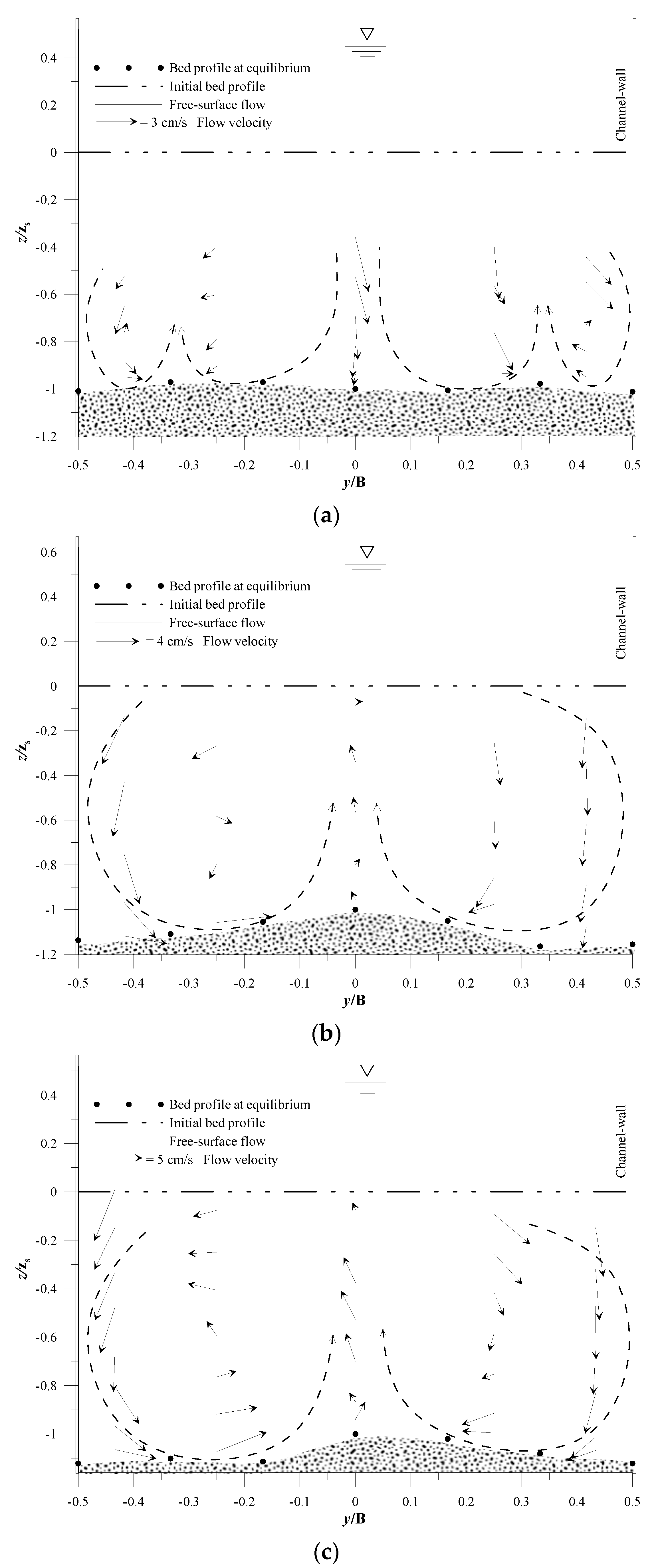
Figure 2 shows examples of the flow velocity distribution,
Vyz, across the equilibrium scour hole at
xs for tests T10, T12, and T13. The
Vyz velocity is the resultant of the span-wise
V and vertical
W time-averaged velocity components. The profiles of the free surface flow (solid line), the initial bed (dash-dotted line), and the bed at the equilibrium state (bullet) are also reported in
Figure 2. The rest of the sediment at the channel bottom is indicated by a random point cloud. The transversal position
y is normalized by the channel width
B, and the vertical position
z is normalized by the maximum scour depth at equilibrium
zs. In
Figure 2, the coordinates
y and
z originate from the channel axis (
y/
B = 0) and the initial bed profile (dash-dotted line), respectively. The maximum scour depth
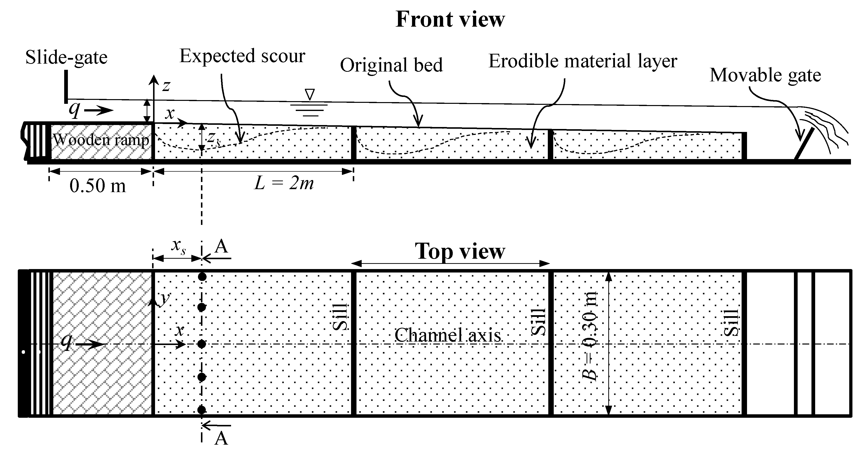
zs is determined based on the longitudinal profile of the equilibrium scour at the channel axis (
y/
B = 0), downstream of the wooden ramp (
Figure 1). The absence of velocity measurements in the upper flow region is due to the limitation of the ADV down-looking probe, being that the uppermost 7 cm of the flow could not be sampled.
To investigate the hydrodynamic structure across the scour hole well, a high-resolution time series of the flow velocities with high quality is required. The magnitudes of the flow velocity vectors reported in
Figure 2 are the result of over 4500 measurements of the instantaneous velocity components.
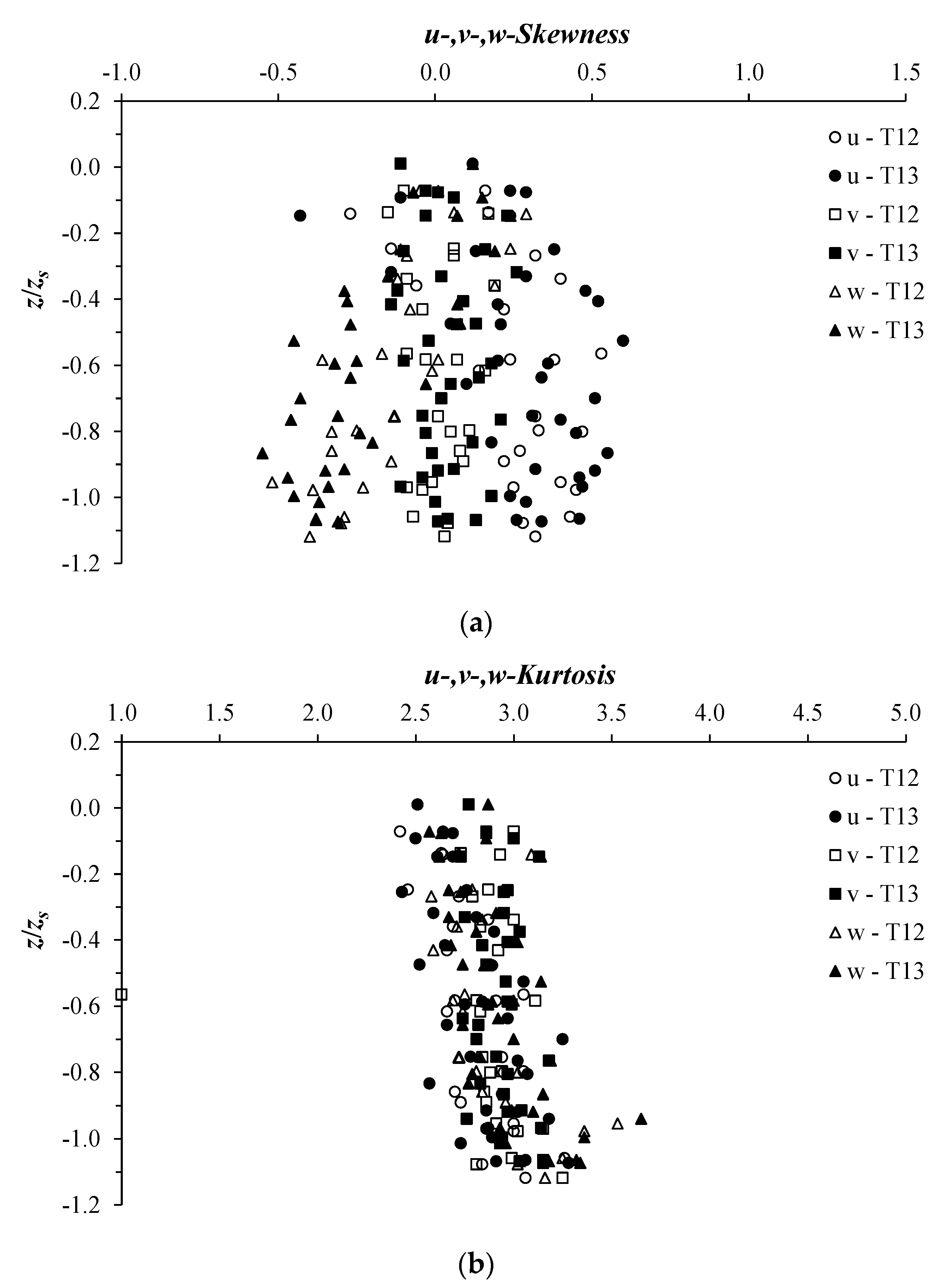
Figure 3, as an example, shows the velocity skewness and kurtosis distribution of all measured velocities across the scour hole at
xs for tests T12 and T13.
Figure 3a shows that the skewness of the three velocity components
u,
v, and
w was between −0.5 and 0.5 in most measuring positions. This implies that the measured velocity data were symmetrical.
Figure 3b shows that
u,
v, and
w kurtosis saturated to a value around 3. These results are similar to the Gaussian case (skewness = 0 and kurtosis = 3), indicating that most of the values of each measured velocity component clustered around the mean value, which means that the ADV instrument was performing satisfactorily.
In
Figure 2, the flow velocity distributions in the scour cross-sections (looking downstream) clearly show the development of secondary current cells. The secondary current cells represent a circulation of fluids in the plane orthogonal to the axis of the primary flow.
Figure 2 shows the formation of a helical motion rotating in opposite directions, as indicated by the curved arrow made of dashed lines in the figure. For test T10,
Figure 2a shows the formation of a series of secondary current cells across the scour hole, similarly to what happens in large straight channels [
20]. The four helical cells shown in the figure are symmetric with respect to the (
x,
z) plane at
y/
B = 0 (plane of flow symmetry).
Figure 2a also shows an undulating sediment profile (manifested by two sediment ridges at
y/
B = −0.25 and 0.25) in the transverse direction. According to previous studies [
20,
21], the undulating sediment profile, generated by secondary current cells, may affect both the whole depth-flow field and the free surface flow pattern.
Figure 2b,c indicates the formation of only two large counter-rotating vortices and a single sediment ridge, located around the channel axis (
y/
B = 0). For tests T12 and T13, the vortices pushed the water outward (towards the channel wall) in the upper part of the scour cross-section, while, near the bottom, the water was driven inward [
19], forming the sediment ridge at the center of the channel. According to previous studies (e.g., [
20,
21]), the hydrodynamics of secondary currents is strongly influenced by the aspect ratio,
Ar (
Table 1), and the number of secondary current cells varies in proportion to the latter. This could explain the increase in the number of secondary current cells with test T10, of
Ar = 2.44, compared to tests T12 and T13, of
Ar = 1.76 and 1.55, respectively.
Figure 2 shows that the width of the secondary current cells is 0.6
hs, 0.9
hs, and 0.8
hs with tests T10, T12, and T13, respectively. This finding agrees with that found in previous studies [
20,
34], claiming that the width of secondary current cells scales with the flow depth.
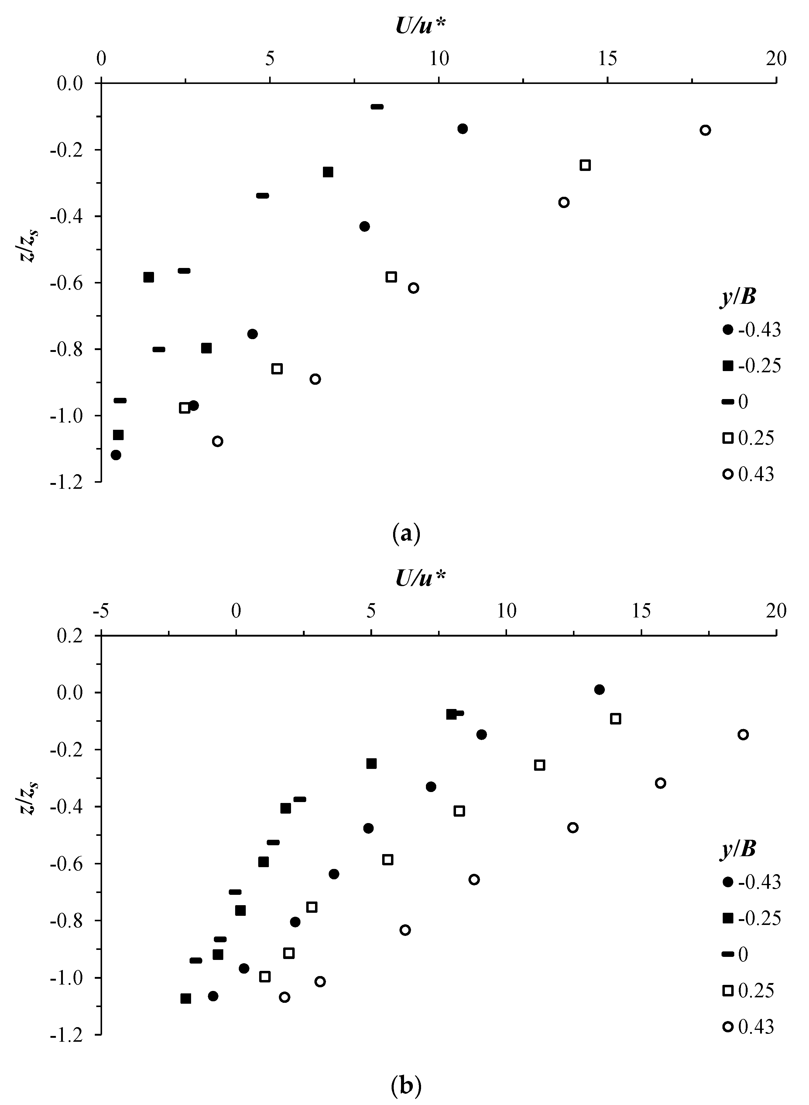
Figure 4 shows the vertical profiles of the normalized velocity
U/
u* at the transversal positions
y/
B = −0.43, −0.25, 0, 0.25, and 0.43 across the scour hole at
xs. Here, the friction velocity
u* was determined based on the measured primary Reynolds shear stresses
U′W′ near the scour bed, and
Z/
hsy < 0.2,
u* = (−
U′W′)
0.5,
Z, and
hsy are defined below. The vertical position
z is normalized by
zs, and originates at the initial bed profile, as shown in
Figure 2. The data refer to test T12 (
Figure 4a) and test T13 (
Figure 4b). At the different transversal positions
y/
B,
U/
u* shows the same trend along the vertical. It is considerably reduced approaching the scour bed. For both tests, the profiles of
U/
u* are shifted from each other, indicating an anisotropic transversal distribution. At the downwelling flow regions, at
y/
B ≤ −0.25 and
y/
B ≥ 0.25 (see
Figure 2), the stream-wise velocity shows the largest values, while it is reduced at the upwelling flow region, around
y/
B = 0. This result is in good agreement with that found by Albayrak and Lemmin [
20] and Stoesser et al. [
27], confirming the significant influence on the primary flow by the secondary current cells.
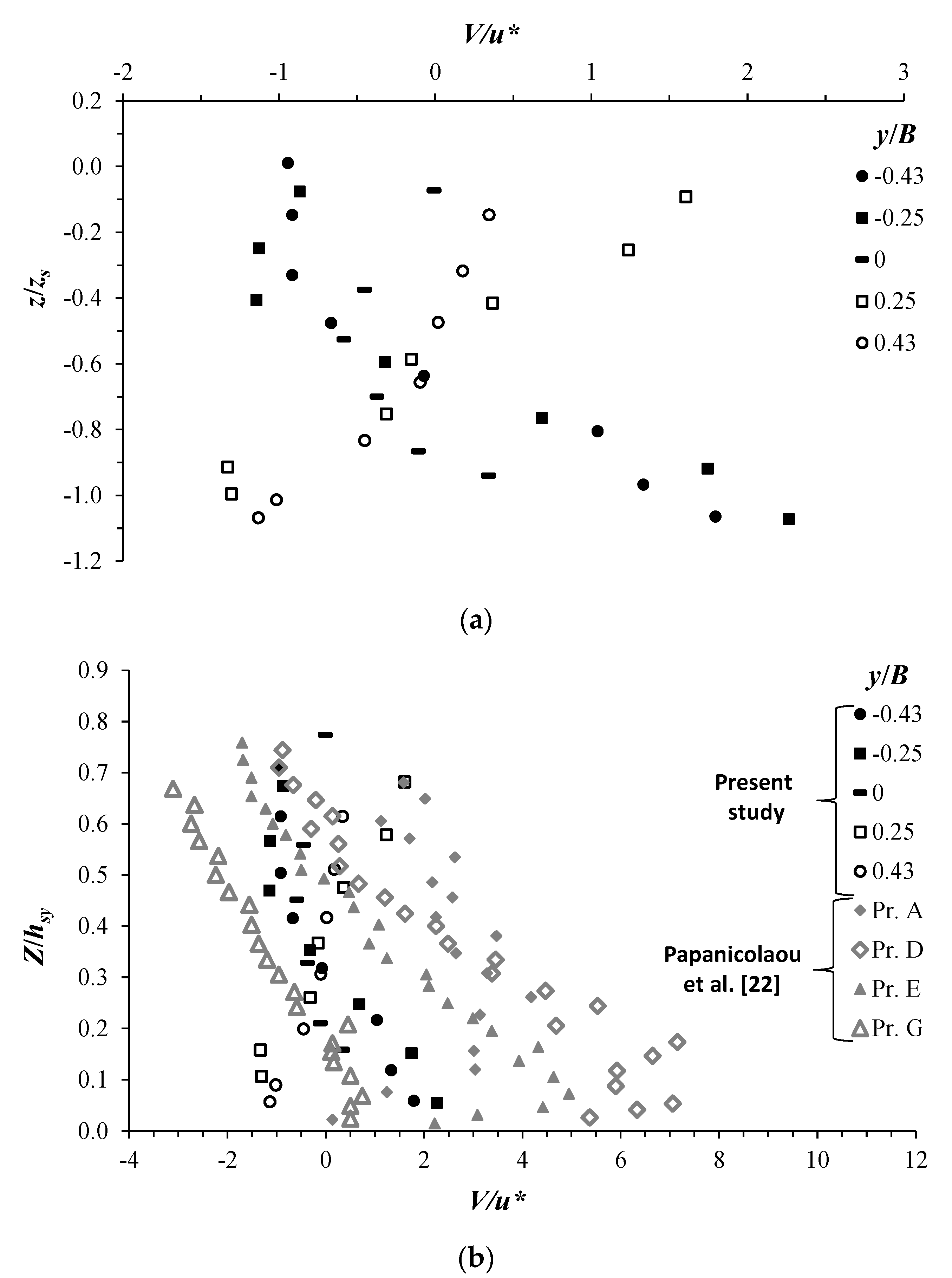
Figure 5a shows an example of the normalized span-wise velocity distribution
V/
u* at the transversal locations
y/
B = −0.43, −0.25, 0, 0.25, and 0.43, across the scour hole at
xs. For the sake of brevity, due to the similar behavior of
V/
u* observed with the different tests, only the profiles of test T13 are included in
Figure 5a. At
y/
B = 0,
V/
u* shows small values tending to zero. This is consistent with the fact that, in the plane of flow symmetry (
y/
B = 0), the transversal velocity component is theoretically null. Moving right or left from the plane of flow symmetry,
V/
u* shows considerable magnitudes. The vertical profiles clearly indicate that
V/
u* changes sign from negative to positive, going towards the scour bed, in the right half of the channel (
y/
B < 0) and vice versa in the left half, forming an x-shape with the different vertical profiles. This behavior of
V/
u* is a result of the development of secondary current cells across the scour hole. The x-shape of the different profiles is due to the symmetry of the vortices with respect to the (
x,
z) plane at
y/
B = 0, as shown in
Figure 2c. To highlight the important role of secondary currents of the second kind in flow dynamics, a comparison of the data in the present study to field data of secondary currents of the first kind, which is usually generated in natural watercourses, is of high interest.
Figure 5b shows a comparison between the vertical
V/
u* profiles of T13, as shown in
Figure 5a, and those obtained by Papanicolaou et al. [
22] on a natural river, characterized by a sequence of channel expansions and contractions along its length. It is worth mentioning that the data of Papanicolaou et al. [
22] were collected along a cross-section of a natural channel of arbitrary geometry (see
Figure 3 in this cited study) without GCS. Seven vertical velocity profiles were taken along the cross-section at different transversal locations A-G, using a SonTek ADV. Analysis of the vector field of the flow velocity,
Vyz, in this cross-section indicates the formation of a single counterclockwise flow circulation, occupying the right half (
y/
B > 0) of the river (see Figure 7 in Papanicolaou et al. [
22]). For the sake of comparison, in
Figure 5b, the vertical position
Z (capital) originates from the channel/scour bed, as in Papanicolaou et al. [
22], and is normalized by
hsy, the local flow depth at a given transversal position
y. Applying the same procedure in normalizing the transverse direction by the width,
B, of the cross-section, as in the present study, where
y = 0 at the center of the cross-section, the profiles Pr. A, Pr. D, Pr. E, and Pr. G, obtained by Papanicolaou et al. [
22], correspond to
y/
B = −0.34, 0, 0.16, and 0.40, respectively.
Figure 5b shows that
V/
u* in the present study behaves quite similarly to that obtained by Papanicolaou et al. [
22]. Moreover, the order of magnitude of
V/
u* within the secondary current cells for both studies seems comparable, as shown by the profiles at the counterclockwise vortices (
y/
B < 0 for the present study and Pr. E and Pr. G in Papanicolaou et al. [
22]). The secondary current in Papanicolaou et al. [
22] (of the first kind) was strongly influenced by the distortion of the primary flow, caused by an upstream bend (convex to the right riverbank) of the channel. The distortion of the primary flow underlies the formation of a single counterclockwise flow vortex, located near the right side of the channel. This could also explain the considerable increase of
V/
u* in the left half of the cross-section at Pr. A and Pr. D (
y/
B = 0), contrary to what happens in the present study conducted in a straight channel, where
V/
u* ≈ 0 at
y/
B = 0, due to the flow symmetry.
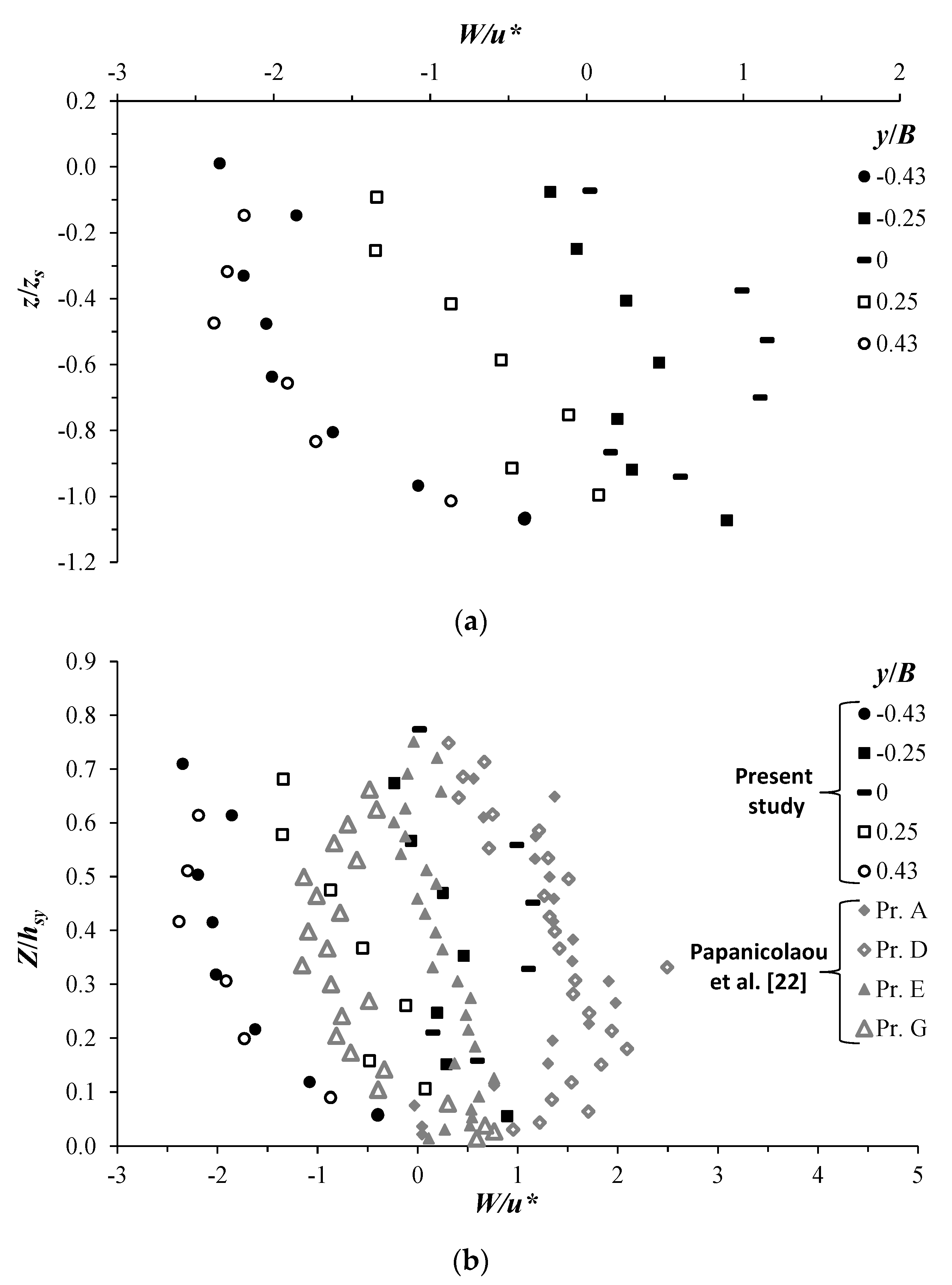
Figure 6 shows the profiles of the normalized vertical velocity
W/
u* for the present study and that by Papanicolaou et al. [
22].
Figure 6a illustrates the profiles of
W/
u* of test T13 of the present study in the scour hole at the downstream position
xs. To clearly show the flow features in the scour hole, we also plotted
W/
u* versus
z/
zs (as explained above). In the downwelling flow regions (
y/
B < −0.25 and
y/
B < 0.25) (see
Figure 2),
W/
u* undergoes negative values, varying in an arched way (of concavity to the right) along the vertical: it increases in magnitude with increasing depth, reaches extreme values of O(−3) at
z/
zs ≈ −0.5, and then begins to gradually decrease (in magnitude), tending toward zero close to the scour bed. In the upwelling flow region (around
y/
B = 0),
W/
u* shows positive values, behaving in a similar fashion (in an arcuate way, but with concavity to the left) along the vertical as in the downwelling flow regions. In the intermediate regions (
y/
B = −0.25 or 0.25, as an example),
W/
u* can change sign from negative to positive and vice versa along the vertical. This behavior of
W/
u* through the scour hole is a result of the flow circulation caused by the secondary current cells.
Figure 6b represents a comparison between the
W/
u* profiles of test T13 of the present study and those by Papanicolaou et al. [
22]. Here,
W/
u* is plotted versus
Z/
hsy (as explained above). The profiles shown in
Figure 6b almost indicate the same order of magnitude of
W/
u* for both studies, ranging between about −3 and 3. At relative transversal positions within a secondary current cell,
Figure 6b also reveals that
W/
u* follows a similar trend along the vertical direction for both studies. The different vertical profiles of
W/
u* relative to a single secondary current cell show a sort of φ-shaped distribution.
4.2. Turbulence Intensities and Shear Stress Across Equilibrium Scour Hole
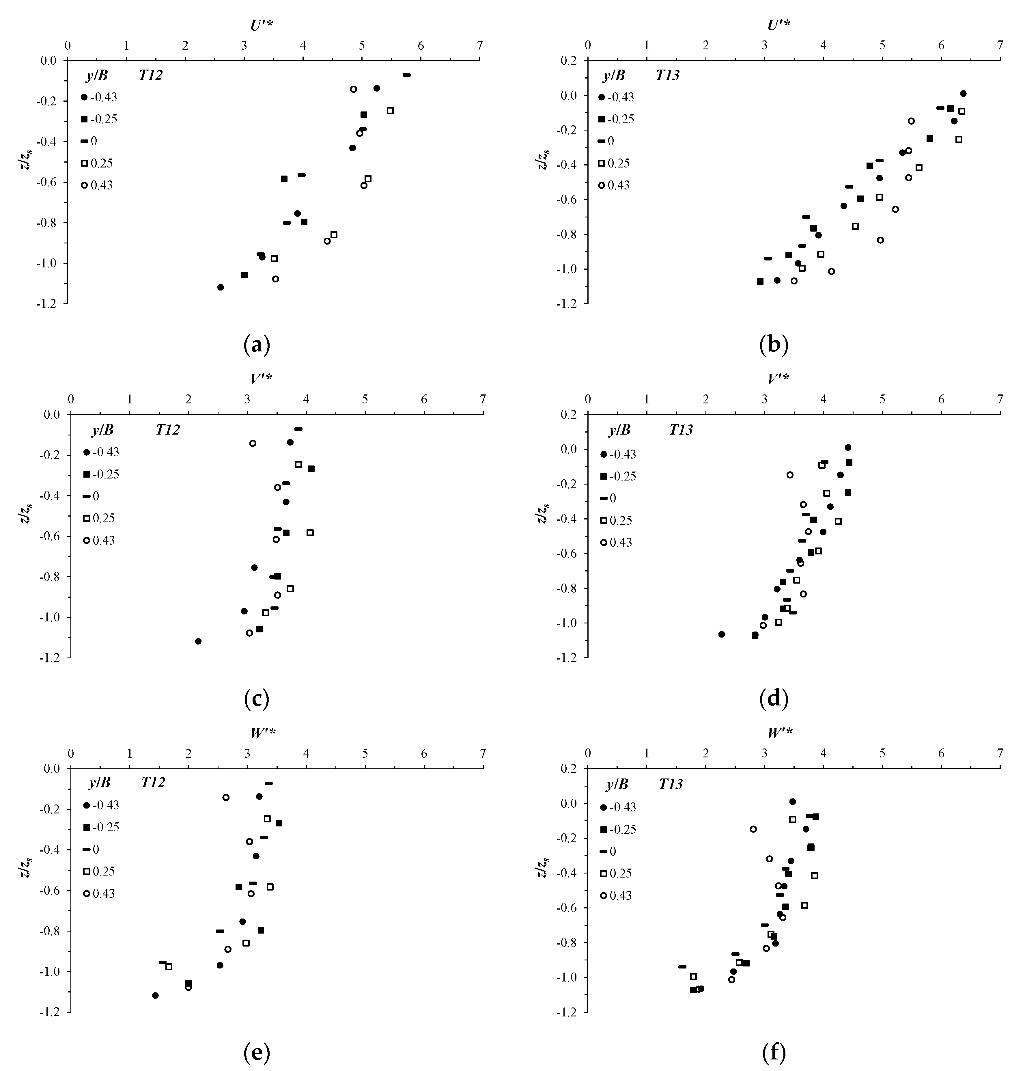
The profiles of the flow turbulence intensities at the different transversal locations
y/
B = −0.43, −0.25, 0, 0.25, and 0.43 across the equilibrium scour hole at the downstream position
xs are shown in
Figure 7. The normalized turbulence intensities in the stream wise direction,
U′*, span-wise direction,
V′*, and vertical direction,
W′* for tests T12 and T13 are plotted in
Figure 7a–f, respectively. Here,
U′*,
V′*, and
W′* are defined as the ratio of the standard deviation of the stream-wise, span-wise, and vertical flow velocity component fluctuations in the friction velocity,
u*, respectively. To show the profiles inside of the scour hole, in
Figure 7, we adapt the normalized vertical coordinate
z/
zs (as explained in
Section 4.1).
Figure 7a,b points out that the stream-wise turbulence intensity generally behaves in the same way at the different transversal locations along the water column in the scour hole.
U′* decreases going down towards the scour from values of O(6) and O(7) at
z/
zs ≈ 0 to values of O(2) and O(3) near the scour bed in tests T12 and T13, respectively. In the upwelling flow region,
U′* decreases almost linearly as
z/
zs decreases. In the downwelling flow region,
U′* decreases in a curved way, which is more pronounced at
y/
B = 0.43. The profiles illustrated in
Figure 7c–f also show, at first glance, a decreasing trend of
V′* and
W′* going to the scour bed. At
z/
zs ≈ 0,
V′* and
W′* have an order of magnitude almost half that of
U′*. Contrary to what happens with
U′*,
V′* and
W’* seem to change more gradually with the distance from the initial bed profile at
z/
zs = 0. Looking closely at
Figure 7c–f, it can be noted that
V′* and
W′* change their magnitudes in an arched way along the vertical; it slightly increases starting from
z/
zs ≈ 0, peaks at almost
z/
zs = −0.5, and then begins to decrease reaching the scour bed. This is more pronounced at the downwelling flow regions, especially with
W′*. The trend of variation of
V′* and
W′* is physically consistent with the behaviors of
V/
u* and
W/
u*, as shown in
Figure 5 and
Figure 6. Similar results of the flow turbulence intensity behaviors were achieved in Chang et al. [
35], studying the scour process downstream of a groundsill.
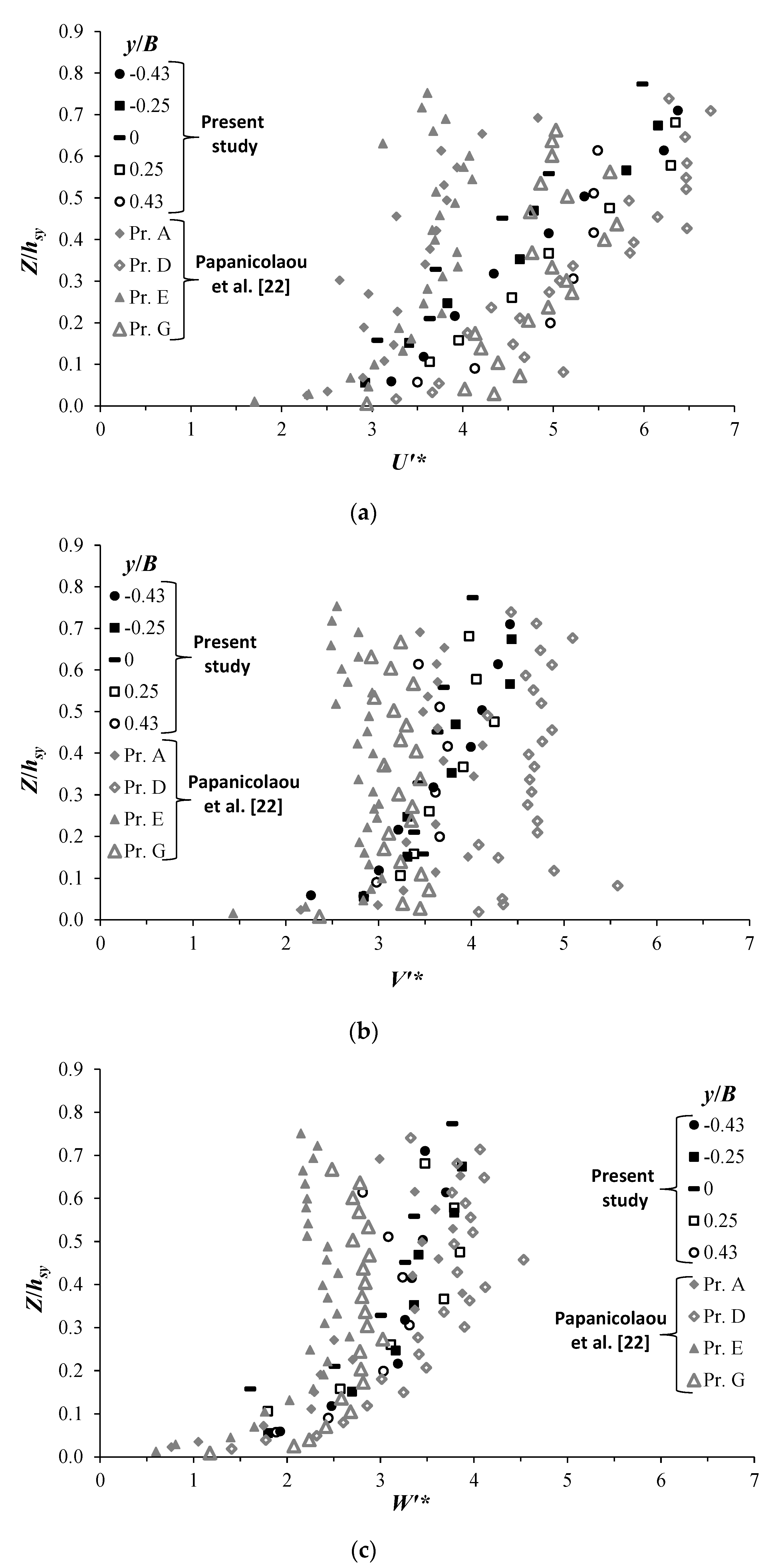
In
Figure 8, we plotted the vertical profiles of
U′*,
V′*, and
W′* of test T13, together with those conducted by Papanicolaou et al. [
22]. Note that, for the sake of consistency between both studies, we adopted in these figures the normalized vertical coordinate system
Z/
hsy. In
Figure 8,
U′*,
V′*, and
W′* show similar trends along the water column. Furthermore,
U′*,
V′*, and
W′* experience quite comparable values, despite the difference in hydraulic and geometric conditions among both studies. A shifting between the profiles of turbulence intensities occurred for both studies, which is pronounced with the data of Papanicolaou et al. [
22], possibly due to the strong bending effect. Contrary to conventional findings in open channels,
Figure 7 and
Figure 8 show that the three turbulence intensities
U′*,
V′*, and
W′* decrease as the channel bottom approaches. This means that the momentum exchange occurs from the bottom towards the surface and not the opposite, as usually confirmed by conventional findings, which may be attributed to the presence of secondary flows [
22].
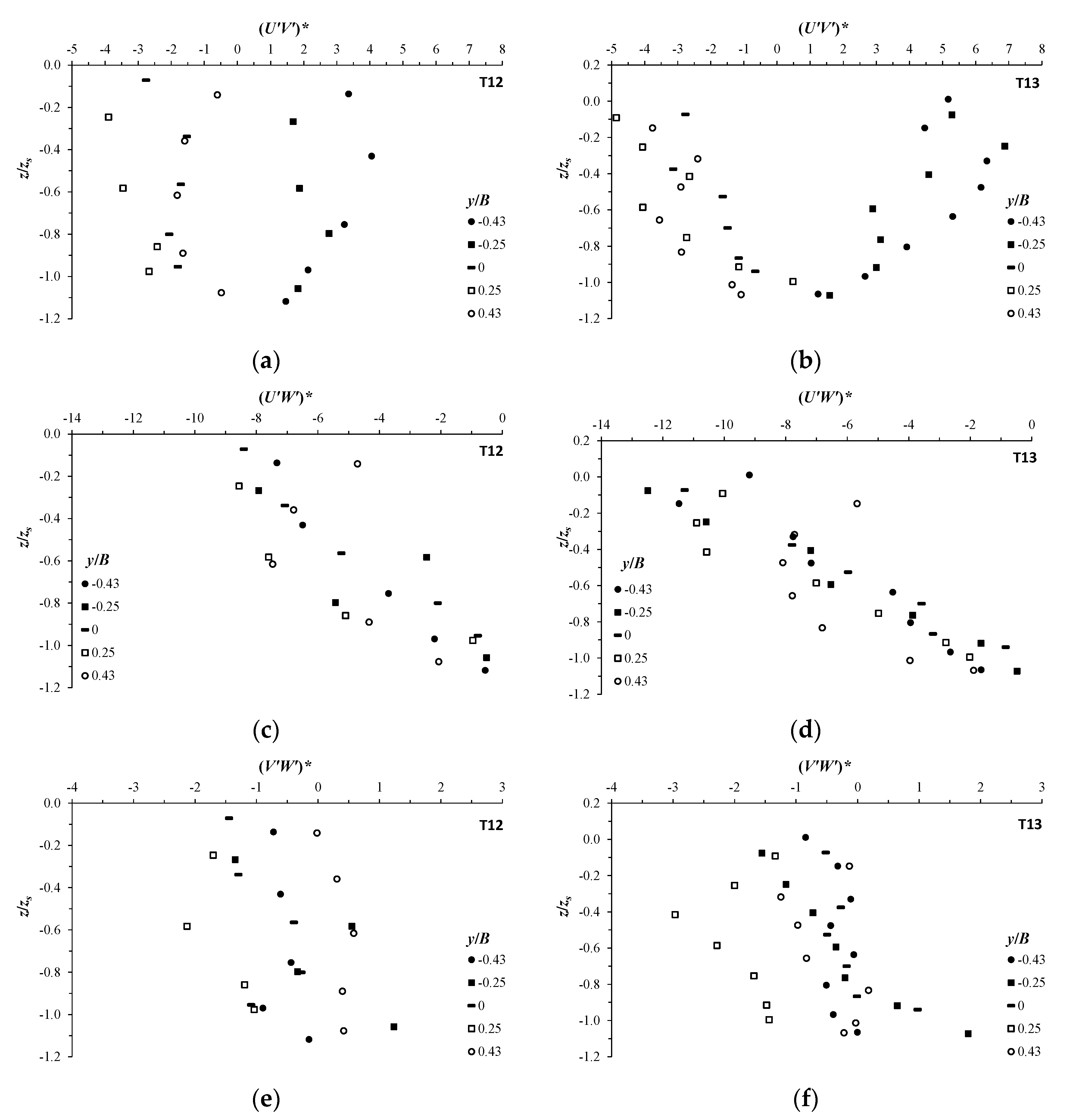
The analysis of the normalized shear stresses across the equilibrium scour hole at
xs was also performed.
Figure 9 reports the vertical profiles of the normalized Reynolds shear stresses at different transversal locations. The measured Reynolds shear stresses,
U′iU′j (see
Section 2) were normalized by the square friction velocity,
u*
2, and for simplicity, they are denoted as (
U′iU′j)*.
Figure 9a,b shows the profiles of (
U′V′)* for tests T12 and T13, respectively.
Figure 9c,d shows the profiles of (
U′W′)* for tests T12 and T13, respectively.
Figure 9e,f shows the profiles of (
V′W′)* for tests T12 and T13, respectively. The shear stresses in
Figure 9 indicate similar behavior to the turbulence intensities. They all show a tendency of decreasing going further towards the scour bed.
Figure 9a,b shows that the span-wise shear stress (
U′V′)* is of considerable magnitudes through the scour hole; it is of magnitudes almost half those of the primary shear stress (
U′W′)*, shown in
Figure 9c,d. The presence of positive and negative values of (
U′V′)* indicates the flow symmetry with respect to the vertical (
x,
z) plane at
y/
B = 0. Theoretically, at y/
B = 0, (
U′V′)* must be null, which is difficult to reach experimentally. The development of secondary currents in the scour hole contributes to a significant momentum transfer in the transverse direction [
27]. The secondary (cross-plane) shear stress (
V′W′)*, as illustrated in
Figure 9e,f, shows the smallest strengths through the scour cross-section, which are two to four times lower than those of (
U′V′)* and (
U′W′)*. By looking at each profile separately in
Figure 9, one can note that the shear stresses show one or more peaks along the vertical, showing in general a curved profile of left or right concave distribution, which agrees well with previous studies (e.g., [
20,
21]).
Figure 9 highlights that the three shear stress components slightly increase when comparing tests T13 with T12, which reflects a proportionality to the Reynolds number
Res (
Table 1).
Figure 9 also points out that the shear stresses (
U′V′)*, (
U′W′)*, and (
V′W′)* exhibit a slight increase in the downwelling flow regions compared to the upwelling regions. This behavior agrees with that observed by Albayrak and Lemmin [
20] in the wall region. Albayrak and Lemmin [
20] noted an opposite behavior, away from the wall region, where (
U′W′)* is larger in the upwelling flow regions than that in the downwelling regions. This may imply, due to the channel’s narrowness in the present study, that the flow in the equilibrium scour hole behaves similarly to that in the wall region in straight open channels with uniform flows (without scours).
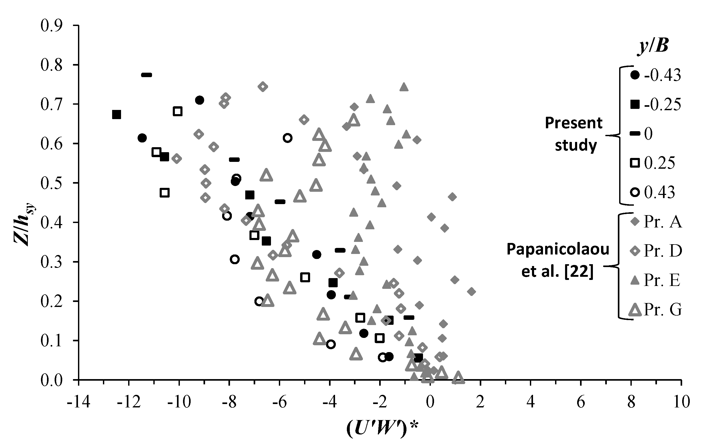
Figure 10 presents a comparison between the shear stress (
U′W′)* of test T13 of the present study and that obtained by Papanicolaou et al. [
22]. Here, we adopt the normalized vertical coordinate system
Z/
hsy (as explained above).
Figure 10 indicates that, for both studies, (
U′W′)* profiles have a similar tendency, especially over
Z/
hsy < 0.3, where the data of both studies tend to collapse together. Furthermore, at
Z/
hsy < 0.3, (
U′W′)* in Papanicolaou et al. [
22] shows the largest strengths in the downwelling regions (Pr. G) compared to that in the upwelling regions (Pr. D and Pr. E). The variation of the Reynolds shear stress values along the transverse direction, between downwelling and upwelling flow regions, reflects the oscillatory nature of the flow induced by the secondary currents, as also confirmed by Albayrak and Lemmin [
20].
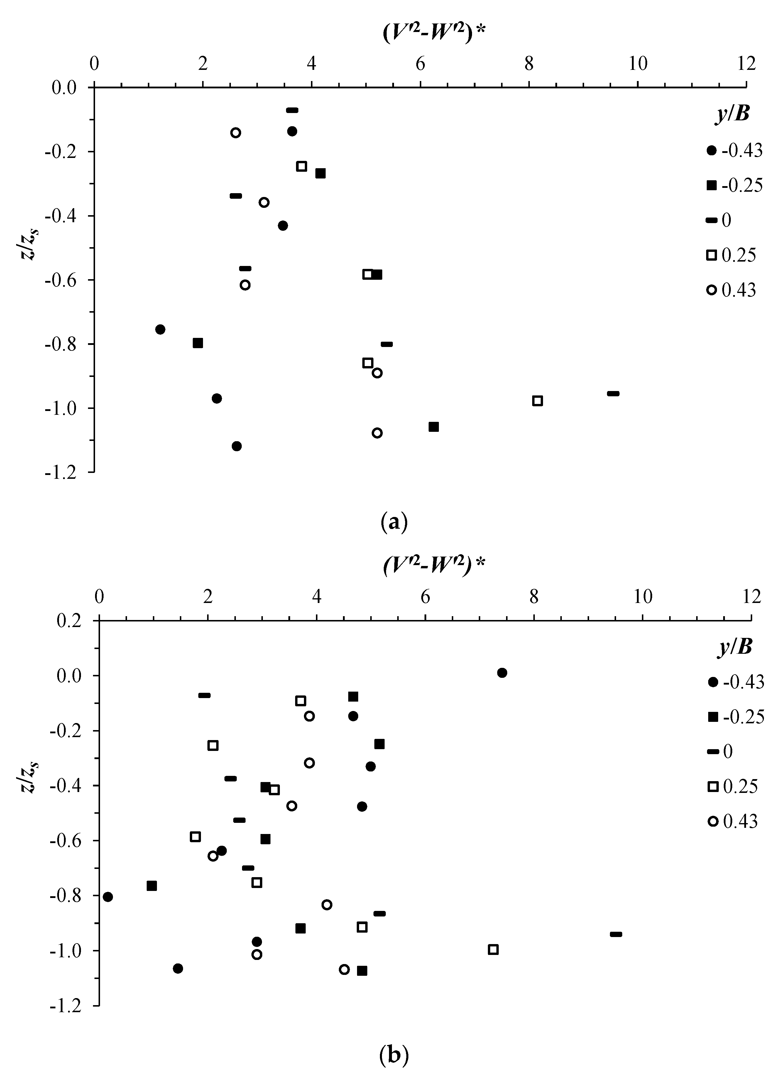
4.3. Contribution of Normal Stress Spatial Anisotropy to Stream-Wise Vorticity
Since the generation of the second kind of secondary currents in the cross-section plane of a straight channel is induced by the inhomogeneity of the Reynolds normal and shear stresses (terms A4, A5, and A6 in Equation (4)), as cited in several previous studies (e.g., [
20,
26]), in
Figure 11, we illustrate the vertical profiles of the anisotropy term of the normal stresses (
V′2 −
W′2)* at different transversal locations
y/
B. Here, by anisotropy, we are addressing the spatial heterogeneities of (
V′2 −
W′2)*. This term is normalized by the square friction velocity as: (
V′2 −
W′2)* = (
V′2 −
W′2)/
u*
2. It is worth mentioning that, according to the literature (e.g., [
28]), the driving mechanism of stress-induced secondary flows only induces secondary currents in straight non-circular turbulent channel flows, not in laminar channel flows.
Figure 11 shows considerable values of the anisotropy term of the normal stresses for both T12 and T13 tests. The profiles of (
V′2 −
W′2)* indicate that the latter varies considerably, both transversely and vertically. This implies the significant contribution of the term A5, as shown in Equation (4), to stream-wise vorticity generation, confirming previous findings in rough-bed, open-channel flows [
27]. By treating each profile separately, it can be noted that (
V′2 −
W′2)* shows a maximum value near the scour mouth, and at
z/
zs = 0, it decreases, reaching a minimum at a vertical position of −0.8 <
z/
zs < −0.6, and then increases, attaining another maximum near the scour bed. This tendency is more pronounced with test T13, and is in good agreement with that shown in a previous study by Stoesser et al. [
27].
For the sake of simplicity, if we neglect all gradients with respect to the stream-wise direction, i.e., ∂/∂
x = 0 (which is physically valid only along a small strip
dx around the downstream location of maxim equilibrium scour depth
xs), the first addends in terms A1 and A3 disappear, while the term A4 vanishes completely. After some additional mathematical operations, the term A2 reduces to zero. After these assumptions, Equation (4) of the mean stream-wise vorticity for turbulent straight non-circular channel flows becomes:
The remaining terms in Equation (5) represent a balance between the convection process (term A1), the diffusion process (term A3), production process (term A5), and suppression process (term A6). The convection by secondary flow serves the transport of vorticity from production regions to the regions of diffusion by viscosity (destruction of vorticities) [
28]. Previous studies [
20,
26] stated that the secondary current is enhanced by the production term A5 and suppressed by the term A6, which are of opposite signs, and are dominant with respect to the terms A1 and A3. Equation (5) reflects the highest importance of the production/suppression processes of vorticity, revealing the critical consideration and analysis of terms A5 and A6.
The comparison between the anisotropy term of the normal stresses (
V′2 −
W′2)*, shown in
Figure 11, and the secondary shear stress (
V′W′)*, shown in
Figure 9, indicates that they have opposite signs, and (
V′2 −
W′2)* has an order of magnitude larger than (
V′W′)*, agreeing with most of the findings in the literature. Furthermore, (
V′2 −
W′2)* shows greater (
y,
z) spatial variation compared to (
V′W′)*, obviously leading to higher gradients. In the literature (e.g., [
26,
28,
34,
35,
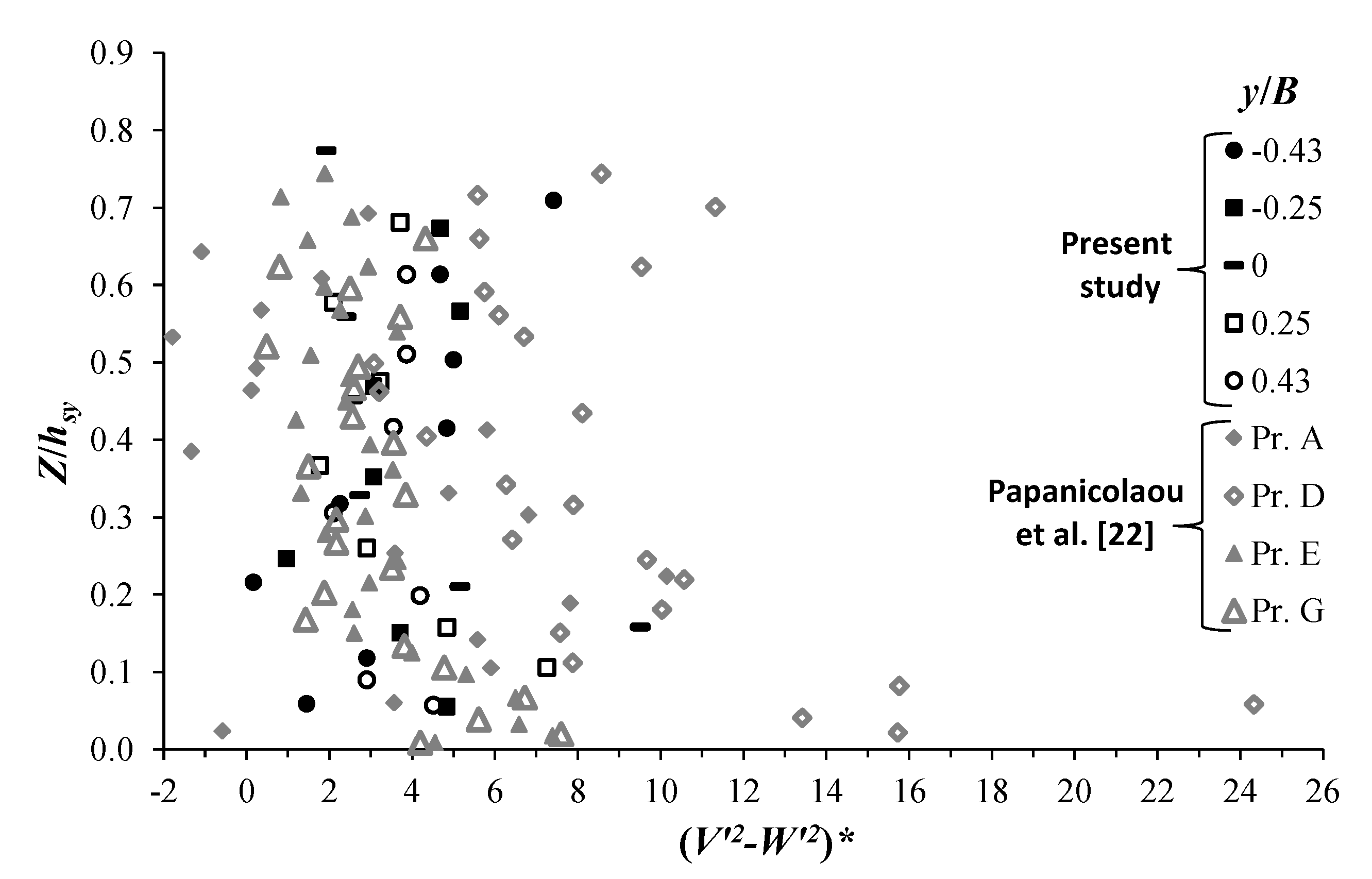
36]), the condition for the generation of a secondary current in straight non-circular turbulent channel flows was considerably discussed, giving rise to two opinion groups. The first group suggested that the anisotropy term of normal stresses, A5, is dominant, providing an essential condition to induce the secondary currents. The second group argued that this term does not play a main role in the generation of secondary currents, but that the latter are the results of the variation of bed roughness or morphology. As indicated above,
Figure 11 shows maximum values of (
V′2 −
W′2)* near both the scour mouth and scour bed, which is more pronounced with test T13 in
Figure 11b. The large values of (
V′2 −
W′2)* in the vicinity of the scour mouth may be the results of high turbulence intensities induced by the incoming jet flow from the grade control structure [
17], while those close to the bed are perhaps enhanced by the deformation of the transversal scour bed and development of sediment ridges [
1,
20,
22]. A significant increase of (
V′2 −
W′2)* near the bed channel is also clearly distinguishable with the data of Papanicolaou et al. [
22], as shown in
Figure 12.
Figure 12 reports a comparison among the data of test T13 in the present study and those of Papanicolaou et al. [
22], plotted with the normalized vertical coordinate
Z/
hsy. Since the secondary currents (of the first kind) in Papanicolaou et al. [
22] were driven by a vortex tilting mechanism due to the channel curvature effect, the presence of high turbulence in the cross-sectional planes, generating an imbalance of normal Reynolds stresses, provides additional driving forces that maintain and enhance secondary flow motions.


