Abstract
An efficient inundation model is necessary for emergency flood responses during storm events. Cellular automata (CA)-based flood models have been proven to produce rapid results while maintaining a certain degree of accuracy. However, the need for computational resources dramatically increases when the number of grid cells increases. Digital elevation model (DEM)-based models generate results even faster, but the simplified governing equations within the models fail to reflect temporal flood evolution. To achieve rapid flood modeling while maintaining model simplicity, a novel two-dimensional hybrid inundation model (HIM) was developed by combining the CA- and DEM-based concepts. Given the temporal flood evolution generated by the CA concept, final finer-scale predictions were obtained by applying the DEM-based concept. The performance of this model was compared to those of widely used, physically based hydraulic models using three UK Environment Agency (EA) benchmark test cases. The HIM yielded consistent prediction results but was faster than the CA-based model. Finally, a comparison was made against flood observations, and the overall root mean squared error (RMSE) for flood depth was 0.388–0.400 m. Considering the uncertainty in the observed flood depths, the HIM shows promising potential to serve as an intermediate tool for emergency response in practical cases.
1. Introduction
Flooding is a major natural hazard that can arise for several reasons, such as reduced river and channel capacity, high rainfall intensity, topography issues, drainage system failure, and storm surges. Floods are among the most devastating natural disasters and cause massive casualties and economic losses [1]. The impact of floods on the global Gross domestic product (GDP) each year amounts to 96 billion US dollars (USD) on average. An average of 21 million people worldwide are affected by floods each year, and this number will rise to 54 million in 2030 due to climate change and socioeconomic development [2]. For these reasons, the prevention and mitigation of flood hazards have become crucial. To support these efforts, a robust and efficient model to predict flood inundation is necessary.
A two-dimensional (2D) hydraulic model solves the 2D governing equations of flow to determine the water depth and depth-averaged velocity on a grid or mesh. The models consider velocity variation on the floodplain and provide flood maps and depth grids as direct outcomes. Therefore, 2D models are suitable for the predictive analysis of a potential flooding situation for emergency response in urban areas. However, applying a 2D hydraulic model to an urban area is complicated and challenging. Detailed settings in 2D models (e.g., drainage and pumping systems, culverts, gates, manholes, etc.) and the need for finer grids for higher-resolution results lead to a high demand for computing power if the response time is limited. Efficiency is also necessary for emergency flood responses during extreme events. To support the evacuation process or rescue operations during flood disasters, decision makers prefer high-resolution forecasts based on current weather conditions within a limited time [3]. If the length of the limited time, named the lead time, is longer, the emergency preparedness or response is more comprehensive. Therefore, an efficient flood model must provide results in a rapid manner so that decision makers can have as much lead time as possible. Thus, developing robust and efficient inundation models has become an important research topic in recent years. Models such as TELEMAC [4], InfoWorks ICM [5], MIKE FLOOD [6,7], HYDRO_AS 2D [8], and NUFSAW2D [9] use shallow water equations (SWEs) to simulate flood inundation. These models provide detailed and accurate results but are computationally expensive because of the internal complexities and associated governing equations. Many physically based models have benefited from efficient solutions since hardware capable of parallel computation (e.g., the GPU) is currently available and parallel computing techniques are rapidly advancing [9,10,11]. Although the computation time has been reduced, these types of models cannot fully utilize parallel processing [9,12]. Moreover, these tools require highly trained personnel to successfully build a model and smoothly run the simulation. This becomes an obstacle when seeking to easily distribute these models to those in need. Another approach to reducing the computation time is to suppress or neglect less important terms within the SWEs for different purposes. For example, the inertial terms are less than the gravity, friction, and pressure terms and can be neglected in the SWEs. This approach can be used to simulate inundation in urban areas [13]. Models such as LISFLOOD-FP [13,14,15], JFLOW [16], and Urban Inundation model-UIM [17] were developed based on simplified versions of the SWEs. These models successfully decreased the computation time while still giving acceptable results. However, for finer-resolution (1–10 m) grids, to maintain numerical stability, the simulation cost is increased by several orders of magnitude due to the smaller time step [15]. It turns out that the full 2D models show better performance in terms of efficiency. As a consequence, solving SWEs, even in their reduced complexity formulations, is still computationally expensive. Parallel computational techniques or high-performance computing (HPC) are still required to cope with this issue [16,17,18,19].
In recent years, many studies have focused on developing simple 2D flood models using the cellular automata (CA) approach [20]. This discrete and abstract computational system introduced by Wolfram [21] has been proven to be faster than physically based models in various applications. This approach considers three fundamental aspects: the world, transition rules, and agents. The world is the place in which the agents reside. In terms of the inundation model, the world could be described as a digital elevation model (DEM), and the agent is water. The evolution of each agent within a cell (central cell) is defined by a set of transition rules and the neighborhood system (NH). The concept of CA has been widely used in several fields; examples include urban growth [22,23], wildfire propagation [24], debris flows [25,26,27], and transportation engineering [28]. In the application of flood simulation, Dottori and Todini [29,30] first applied the CA model to develop a storage-cell-like flood model. Later, many algorithms focusing on the transition rules were developed, such as the ranking system [31], minimization [32,33], weighted parameter [12], and motion cost field [34]. All of the abovementioned CA models rely on similar definitions of state variables but differ in the formulation of the fluxes [20]. Although these methods can reduce the computation time, applying the algorithms for each cell is still a burden, especially when the number of cells is massive or for complex terrain shapes [35].
Other researchers have used a very different approach as an alternative to rapidly simulate floods in urban areas with high-resolution DEMs. The approach is based on the topography of the area. It is assumed that floodwater always fills the depression storage within the area and that the water surface remains flat when it reaches equilibrium. This kind of approach considers the continuity equation to predict the maximum inundation (GUFIM by Chen et al. [36]; ISIS FAST by CH2M [37]; SPM by Yang et al. [38]; RUFIDAM by Jamali et al. [39]. This concept type is considered a DEM-based concept hereafter in this paper. By neglecting the complicated momentum equations and the temporal variation in flooding (Δt), these models can rapidly provide maximum water elevation or water depth predictions. The computation time is short, but data processing time is needed. These types of models require DEM pre- and postprocessing to generate inundation maps. The time to execute these steps is dependent on various factors, such as user capability, study area size, and grid resolution. For example, these steps can take up to 2–10 min for DEMs covering an area of 0.8 to 10 km2 with a 1 m resolution [39].
In terms of accuracy, physically based models are the best choices for applications. Solving SWEs is challenging and computationally costly, particularly for the large domains typical of hydrological problems [40]. The same issue can also be found in CA models. Although the drawback in computation time can be addressed by using parallelism or HPC, in practice, not all sites have the budget or personnel to operate such complex models. On the other hand, the DEM-based approach provides rapid results but lacks detail. For example, the temporal evolution of flooding, which is very important for decision-making, cannot be modeled in the DEM-based approach.
This study proposes a novel hybrid approach that integrates CA- and DEM-based flood models to provide a detailed inundation map with acceptable accuracy and efficiency for emergency purposes without excessively complex mechanisms. The objectives of this study are (1) to seamlessly combine CA- and DEM-based models to generate efficient and operational flood forecast information and (2) to develop an easy-to-use tool that can help quick decision-making for flood preparedness and response.
2. Hybrid Inundation Model
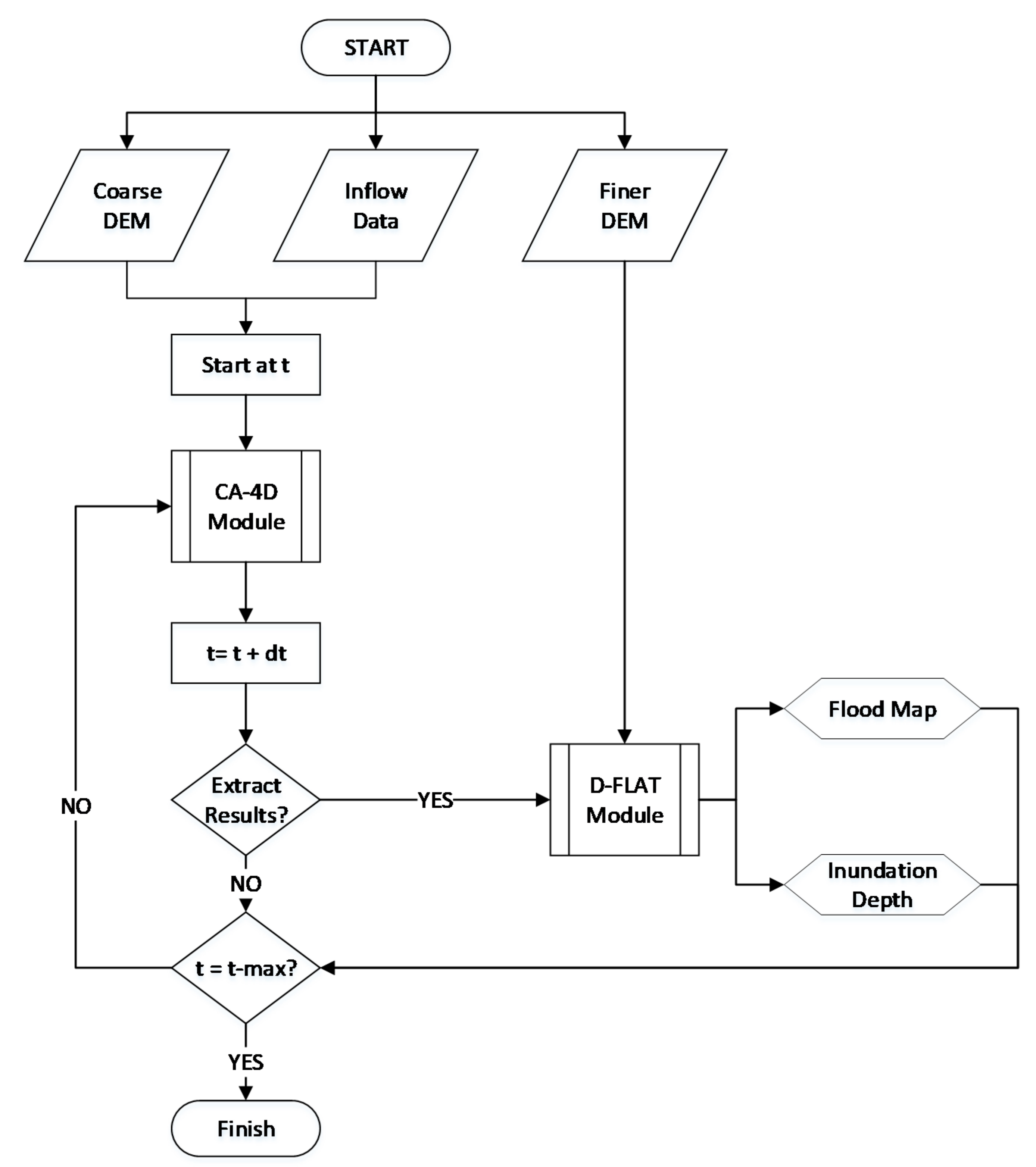
The purpose of this study is to develop a model that can provide fast and accurate enough results for emergency purposes while maintaining simplicity in operation. The proposed hybrid inundation model (HIM) utilizes two models, the CA-4D model and the D-Flat model, which are described in the next section. The basic idea of the HIM is to let the CA-4D model calculate the water depth for the next time step using a coarse grid (e.g., 5 m and coarser). If the marching time reaches a certain time to extract or save the results (e.g., a user-defined value, usually every 5 or 10 min), the results from CA-4D at that specific marching time will be transferred to the D-Flat model. For the next step, the D-Flat model interpolates the results from CA-4D and generates a higher-resolution (e.g., 2 m and finer) inundation map. The concept is similar to the concept of the subgrid method used by different studies [41,42,43,44]. In these studies, the subgrid method addressed the disagreement between topographic data resolution and model grid resolution. A flood model can use this method to run simulations with a coarser grid resolution while producing a solution with a finer grid resolution. Using the subgrid method, faster computation time is achieved by performing fewer flux computations in each time step. Additionally, a higher time step can be used without destroying the model stability. This approach has been intensively studied for the last decade, especially for SWE models. However, the proposed HIM used a different concept from the subgrid approach. For example, HIM does not derive or discretize any equations into subgrid solutions as the subgrid method does. Instead, HIM uses the outputs from the CA model with coarse grids as input for the DEM model with finer grids. The workflow of the HIM is shown in Figure 1. In the figure, the flood map is the inundation extent, while the inundation depth is the water depth for each grid cell. Overall, the HIM can be defined as a CA model that works in conjunction with subgrid-scale interpolation strategies to generate higher-resolution results. For preliminary analysis, the model was designed to work with rectangular grids with the von Neumann NH system. The details of this new model are described as follows.
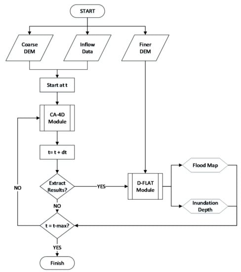
Figure 1.
Flowchart of the HIM.
2.1. Cellular Automata 4-Direction (CA-4D) Model
The CA-4D model uses the von Neumann NH system. This means that a square grid DEM is applied. A central cell is considered to calculate flood exchange between its four cardinal adjacent cells. The basic principle of the CA-4D model uses the zero-inertia equation as the governing equation. Although some other models, such as the raster-based storage model LISFLOOD-FP [14] and the model proposed by Dottori and Todini [29,30], also use similar principles, some aspects are different. The difference is addressed below. CA-4D assumes that the change in cell volume over time is equal to the fluxes in and out of the cell during the time step (Equation (1)). However, CA-4D considers only water flow out of a cell, while water flowing into the cell can be treated as water flowing out of the neighboring cells. This assumption can speed up the calculation process. The calculation is repeatedly performed for each cell until equilibrium is reached. It is not necessary to address water flowing in/out of the same cell. Manning’s equation is used to calculate the flow rates between cells (Equation (2)).
where QNH (m3/s) denotes the flow rates from the central cell to the NH, M is the total number of cells in the NH, WS0 (m) is the water level in the central cell, WSNH (m) is the water level of the NH analyzed, n is the Manning roughness coefficient (m−1/3s), dx is the grid size (m), hNH (m) represents the depth at which water can flow between the central cell and NH cells, and Z0 and ZNH are ground elevations (m) for central and neighboring cells.
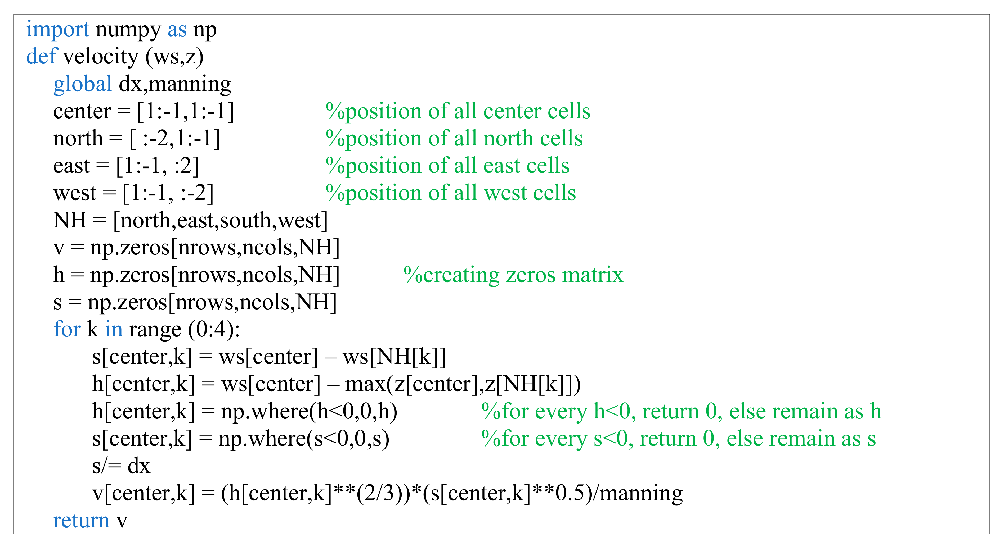
Python is arguably not the most efficient programming language to perform this type of simulation. For example, to calculate Equation (1), the algorithm considers each cell and its corresponding calculations sequentially. This technique is slower in the Python language than in other programming languages (e.g., Fortran). This disadvantage could be solved by implementing multiprocessing computation or applying other more efficient programming languages. However, since the aim of this model is to maintain simplicity, CA-4D uses another technique to make the calculation more efficient. Instead of performing the calculations sequentially, CA-4D utilizes the Numpy library functions in Python and solves the equations using matrix-like operations. By simply changing the techniques, the computation can be made up to 30 times faster for each loop. Figure 2 shows an example of pseudocode to perform the matrix-like operation to calculate the velocity.
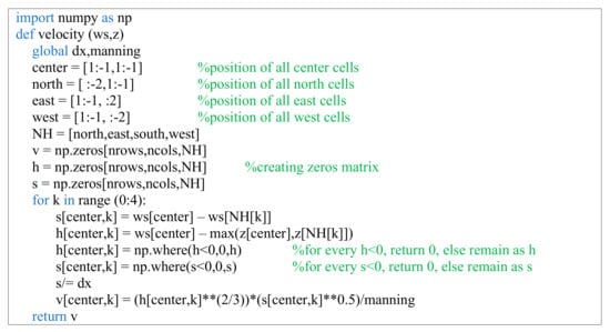
Figure 2.
Pseudocode for calculating velocity by using the Numpy function library. Python functions are shown in blue, and comments are shown in green.
Once the flow rates are determined, the adaptive time step is calculated to update the water surface elevation. Given that CA-4D is a diffusive-like model, the most stable time step equation is that provided by Hunter et al. [15]. However, that study found that the corresponding formula is computationally expensive. Thus, the CA-4D model uses a different approach to calculate the adaptive time step by using the simple Courant-Friedrichs-Lewy (CFL) condition:
where Δtlim is the minimum time step set by the users, and α is a coefficient used to maintain simulation stability for most flow conditions. The parameter α is included because the stable time step is often less than that indicated by the CFL condition. Instead of finding the most stable time step value by using a complex equation, in which the time step decreases quadratically as the cell size decreases, α is introduced to reduce the time computation complexity. Vmax is the maximum of the wave celerity c and water velocity Vi to the surrounding cells. The stable time step in the zero-inertia model is required to ensure that oscillation chequerboard does not occur and destroy the results. Unlike the equation proposed by [15], which sometimes returns a very small dt to ensure stability, the CFL stability criterion allows some flexibility. For emergency purposes, where time is essential, a higher value of α could be chosen to obtain a larger time step. Of course, oscillation likely occurs as a result. However, if the oscillation does not destroy the whole solution, it could be treated as data noise. Furthermore, when time is not an issue, α could be set lower to produce more stable results.
In the CA-4D model, the water depth is updated by subtracting the outflow volume from the water depth of the current time step. Then, the water depth of the NH should incorporate the outflow volume from the central cell. Furthermore, the water depth of the next time step is updated with any lateral inflow or outflow (e.g., rainfall and losses). CA-4D applies two rules to prevent more water from leaving the central cell than it contains and to prevent adding more water to the NH cell than it should. Under normal conditions, the water volume leaving the central cell is less than or equal to the central cell’s available water (AW) volume. Equations (6) and (7) are used to update the water depth:
where (m) is the updated water surface elevation of the central cell at the next time step, (m) is the central cell water surface elevation at the present step, (m2) is the area of the cell, (m3/s) is the outflow from the central cell to the NH cell, (m3) is the lateral input volume of water into the central cell (e.g., precipitation, drainage overflow, or discharge from the upstream area), and (m3) is an outflow volume of water from the central cell (e.g., outflow to the downstream catchment or lateral outflow). However, under certain conditions, more water leaves the central cell than is available. The water is distributed to the NH cells proportionally according to the water flux rates. Equations (8) and (9) are used to update the water depth for the extreme condition:
where (m) is the maximum intercellular depth allowable into the NH. In this case, is equal to the maximum .
2.2. DEM Based on the Flat-Water Assumption (D-Flat) Model
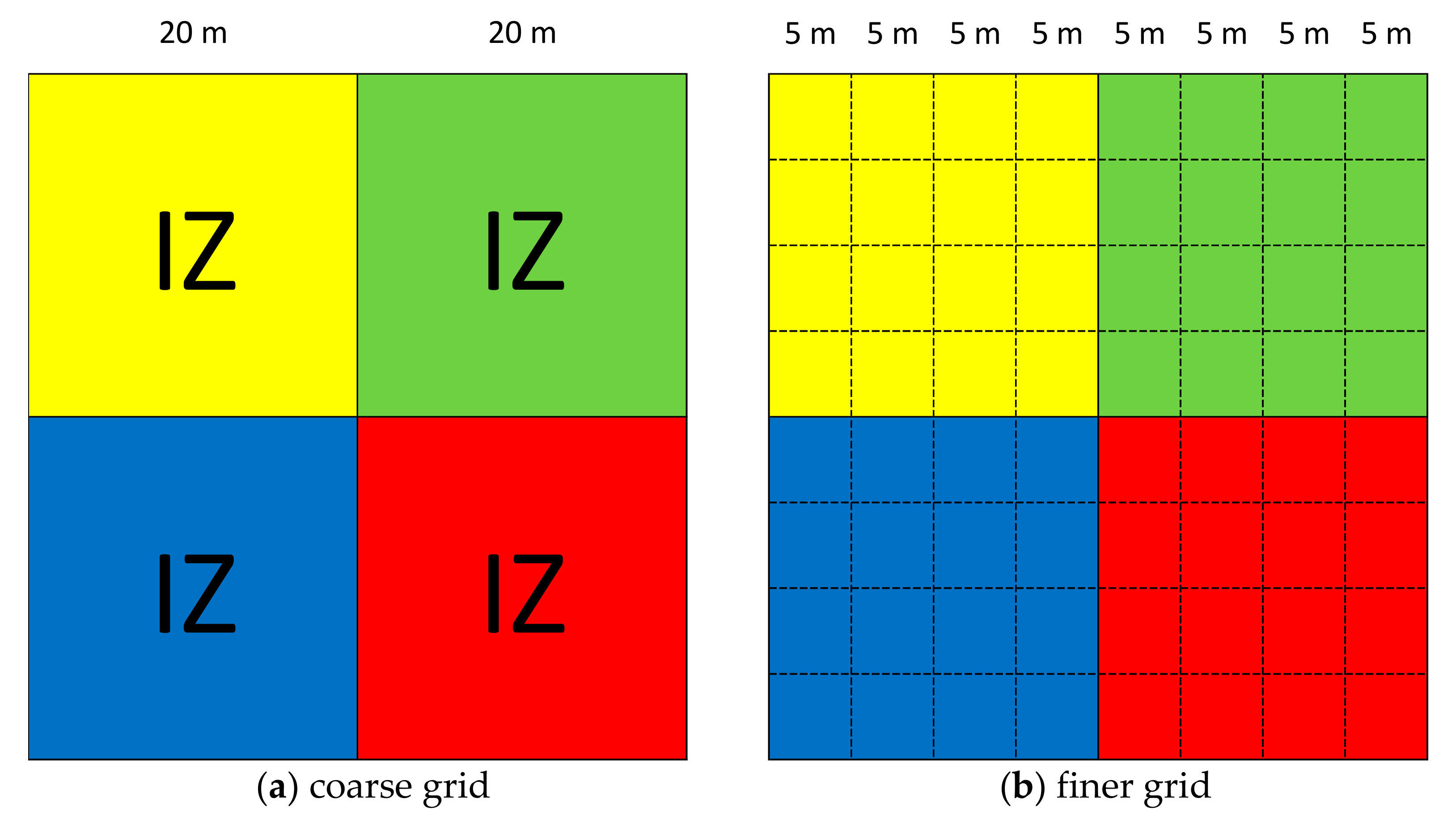
After updating the water surface elevation in the CA-4D model, the water volume in each coarse grid cell is redistributed into finer grid cells by using the D-Flat model when the user-defined timestep is reached. The proposed hybrid model uses the coarser-grid DEM as an impact zone (IZ, a boundary) for the finer-grid DEM to generate the high-resolution inundation map. The IZ is defined as a boundary where the volume could only be redistributed within the same boundary. Figure 3 shows an illustration of the IZ. The water volumes generated from the CA-4D model in the coarse grid with a certain color (e.g., red) can only be redistributed to the finer grid with the same color.

Figure 3.
IZ illustration. The block of cells on the left (a) represents the coarse grid used by the CA-4D model. Each coarse grid cell acts as an IZ for the finer grid (b) used by the D-Flat model.
As its name suggests, this model uses a flat-water assumption to distribute the water. This assumption is used not only because it provides the fastest computation with reasonable results but also because in a sufficiently small area, the major driving force to control floodwater is assumed to be gravity only [36,38]. The water distribution from coarse to finer grids is explained in Figure 3. The water volume from the coarse grid is distributed to the finer grid with the same color. In other words, the coarse grid acts as an IZ in the finer grid. Hence, the preprocessing step that generates the IZ can be neglected.
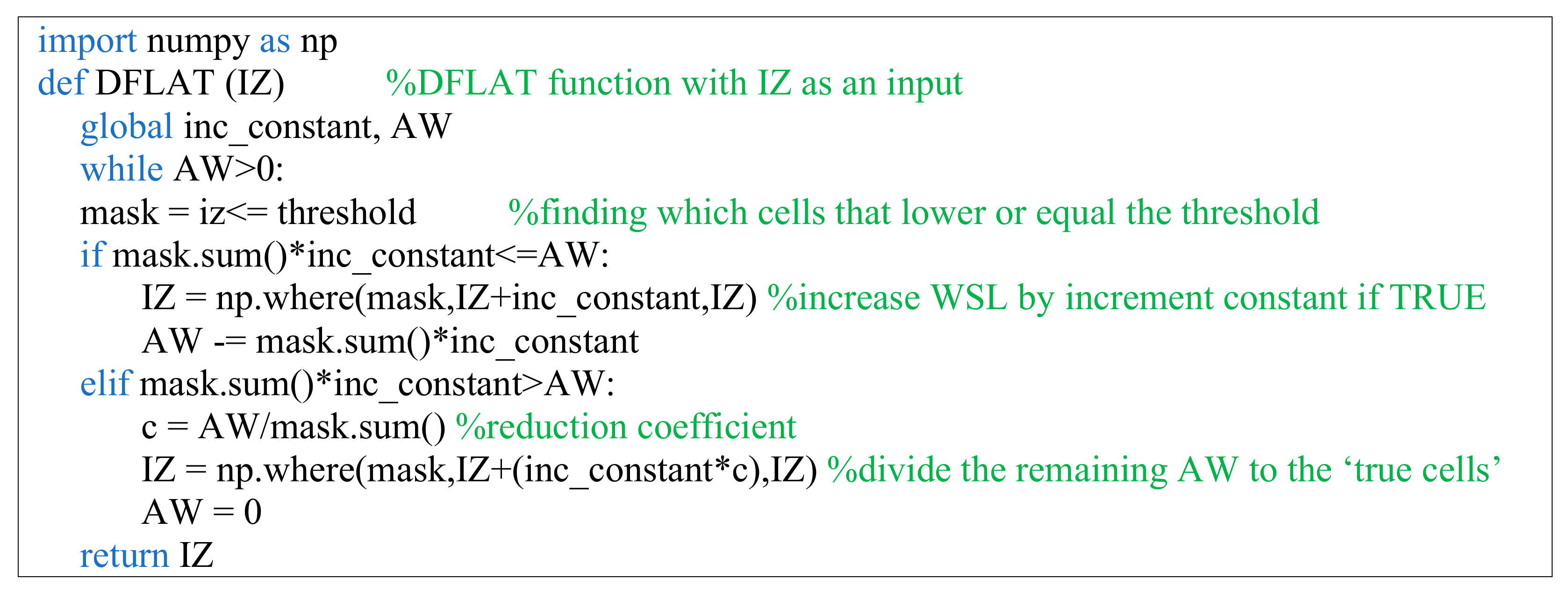
The basic idea of this model is to find the cell with the minimum elevation as the starting point and increase its elevation by a constant increment. This process is repeated until no more water is available to be distributed. However, this approach may not be able to spread the water within the IZ if the ground slope is very steep, causing the water to accumulate in only one cell. To prevent this, the threshold value is determined by averaging the minimum and maximum ground elevations within an IZ. Every cell within the IZ that is lower than or equal to the threshold is indicated as the starting point (‘true cell’). As shown in Figure 4, the D-Flat model starts by counting how many cells are lower than or equal to the threshold value (true cells). These true cells are determined as route-starting cells in which the constant incremental filling starts. To ensure mass conservation, before the water is distributed, the model calculates how much water is to be distributed by simply multiplying the constant increment by the number of true cells. If the outflow is less than the AW, then the number of true cells is increased by a constant increment. If the outflow is more than the AW, the AW instead of the outflow is distributed equally to the true cells.

Figure 4.
Pseudocode for distributing the water volume within the coarse grid cells to the finer grid cells. The IZ parameter refers to the ground elevation within the IZ.
Extreme rainfall is the major factor that causes floods. Earth Scientists uses a concept called connectivity as a means to describe the origin of floods, and this concept is associated with the fluxes of water and sediment on different scales: aggregate, pedon, location on the slope, slope, watershed, and basin [45]. This results in different types of floods, such as fluvial and pluvial floods. Floods in mountainous terrain from small creeks, classified as fluvial floods, are also becoming more frequent [46]. However, the abovementioned algorithms are focused on pluvial floods in urban areas. The soil condition was assumed to be fully saturated to obtain the maximum flood extent requiring an emergency response. The concept of equivalent or effective parameters has been used to define the effect of connectivity in this study. For instance, Manning’s roughness coefficients were used to describe roughness, vegetation or an index of connectivity. Differences in the DEM were used to describe the terrain slope and flood water movement.
3. Details of Case Studies
Two kinds of case studies were conducted in this study to evaluate the model performance. One is hypothetical cases applied in the UK for 2D hydraulic benchmark tests, and the other is a historical flood event that occurred in coastal areas of Chiayi County, Taiwan. The details are discussed in the following subsections.
3.1. Three UK EA Benchmark Test Cases
The model developed in this study was applied to three cases from UK EA benchmarking tests (hereafter referred to as the EA benchmark tests) for 2D flood modeling [47]. The EA benchmark test cases have been applied to many 2D hydraulic models to test their capability and performance in response to different types of hydraulic conditions. More information on the test cases can be found in Néelz and Pender [47]. In this work, three cases were selected: Test 2 (EAT2), filling the depression storage; Test 4 (EAT4), flood propagation over a flat area; and Test 8A (EAT8A), flood inundation induced by rainfall and a point source inflow in a small urban area. The other test cases, which were not selected in this study, are either cases in which the 1D channel component is needed (e.g., Test 8B, 1D-2D problem) or problems that the proposed model was not designed to solve, such as Test 3, which requires momentum conservation. Other cases can be applied until further improvements are made in future studies.
No observation data were provided within the cases; however, several models were used to simulate the cases, and the results were compared. To compare the proposed model results, the results of other 2D models were selected: TUFLOW [48] and LISFLOOD-FP [10]. These two models are widely used in the water industry and are among the 2D hydraulic models used in the EA benchmarking exercise [49]. TUFLOW uses full SWEs as the governing equation, while LISFLOOD-FP uses a simplification of the SWEs. For this purpose, three common model performance indicators [50]—namely, (i) the true positive rate (TPR), (ii) the false discovery rate (FDR), and (iii) the root mean square error (RMSE)—were used as the metrics to compare the model results. The equations of the TPR, FDR, and RMSE are expressed as
The true positive (TP) parameter denotes the number of cells that both models considered wet (i.e., inundated). The false-negative (FN) parameter is the total number of cells that the analyzed model identified as dry but the targeted model identified as wet. The false positive (FP) parameter is the opposite of the FN parameter; it represents the total number of cells that the analyzed model identified as dry but the targeted model considered wet. denotes the predicted water depth of the ith cell of the targeted model, denotes the predicted water depth of the ith cell of the analyzed model, and p is the total number of wet cells. All these indicators consider wet cells to be those that have at least 0.1 m of water depth.
3.2. A Historical Flood Event
A low-pressure zone and southwest airstream moved toward southern Taiwan gradually between 23 and 29 August 2018. Over 500 mm of precipitation fell on coastal areas in Chiayi County, Taiwan, in 24 h, resulting in 7 casualties, 8492 people evacuated, and more than 14 million USD in economic losses. A total of 116 locations were flooded. According to a postdisaster report, the intensity of the rainfall exceeded the design capacity of drainage systems and was the major cause of flooding. The coastal areas of Chiayi County and this event were selected as the case study. The RMSE between recorded flood depths, TUFLOW results, and simulated results was used to evaluate the performance of the HIM model.
4. Results and Discussion
4.1. Three UK EA Benchmark Test Cases
Within the first study, two scenarios were analyzed. First, the model was set to act as a fully CA-based model, and in the second scenario, the model was set to act as a hybrid model (i.e., a combination of CA-4D and D-Flat). The purpose of these two scenarios was to evaluate the improved performance of the DEM-incorporating model in terms of accuracy and efficiency.
Table 1 shows the parameters of various simulations used to simulate the EA benchmark test cases. The most important parameter for CA-4D is the parameter α in Equation (4). This value has a significant impact on the actual computation time to finish a run. The parameter α should be low enough to ensure model stability but high enough to ensure computational efficiency. In conclusion, a higher α value returns a coarser precision but with a faster run time. For the hybrid simulation, many parameters must be determined based on professional judgment or trial-and-error rules. An important configuration step is to set the ratio of grid resolution between coarse grid resolution (CA-4D) and fine grid resolution (D-Flat). If the ratio (hereafter referred to as the DEM ratio) is high, the computation time may decrease significantly. The prediction accuracy may decrease for the following reasons. The assumption of flat-water theory in D-Flat is limited to small and flat areas. If the topography of the applied area (i.e., each color block on the right in Figure 3) changes dramatically or the area is too large, the assumption may not be sustained. A higher DEM ratio makes the IZ larger and may cause the D-Flat assumption to not be sustainable. Second, the results of CA-4D serve as input to the D-Flat model in HIM. The CA results have an impact on the prediction accuracy. It tends to oversimplify the topographic effect and provides fewer details by running CA-4D with a coarser grid. In this work, a 4–5 DEM ratio was used. For example, Table 1 shows that a ratio of 5 was applied in the HIM for the EAT2 scenario. This means that an integration of the CA-4D model with a 100 m × 100 m DEM and the D-Flat model with a 20 m × 20 m DEM was considered. The resolution of the final results was 20 m × 20 m, which is consistent with the results of the CA-4D model only. The second important parameter is the output frequency, which determines when the data are being extracted or saved. In the case of the HIM, it is the time when the data from the coarse CA–4D results are interpolated to a finer resolution using the D-Flat model. If a very small output frequency is used, then the computational time will increase due to excessive D–Flat model activation. In this case, the HIM uses the output frequency that is already set consistent with the benchmark. The last important parameter is the increment constant (inc_const). This constant determines how much water is added to fill the lowest elevation within the IZ during each iteration. Selecting a smaller increment constant leads to better performance. However, it necessitates more simulation time. Ref. [50] performed a sensitivity analysis regarding the increment constant. The model performance was found to not improve for increment constants smaller than 0.001 m. Hence, the HIM used 0.001 m as a default value for the increment constant. For both models, a finer grid resolution was used as the final result.

Table 1.
Parameters used in CA-4D and the HIM for the EA benchmark test cases.
The purpose of implementing EAT2 is to evaluate the capability of the model to determine the inundation extent and final flood depth, which involves low-momentum flow over complex topography. The region, as shown in Figure 5a, has an area of 2000 m × 2000 m and 16 locations with ~0.5 m deep depressions. A uniform Manning coefficient of 0.03 was applied to the whole domain, and a 20 m resolution DEM was expected to be used. The initial condition was a dry bed with a closed boundary area. The inflow boundary was applied along a 100 m line running south from the northwest corner, the value of which is given in Figure 5b. The original problem specified 16 output points at the center of each depression, where points 1–4 start from the lower left depressions (X, Y = 250 m, 250 m) to the upper left (X, Y = 250 m, 1750 m).
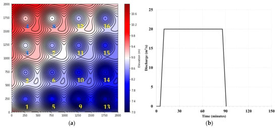
Figure 5.
(a) EAT2 domain with contour lines every 0.05 m (b) Inflow from the northwest point (x, y = 0 m, 2000 m).
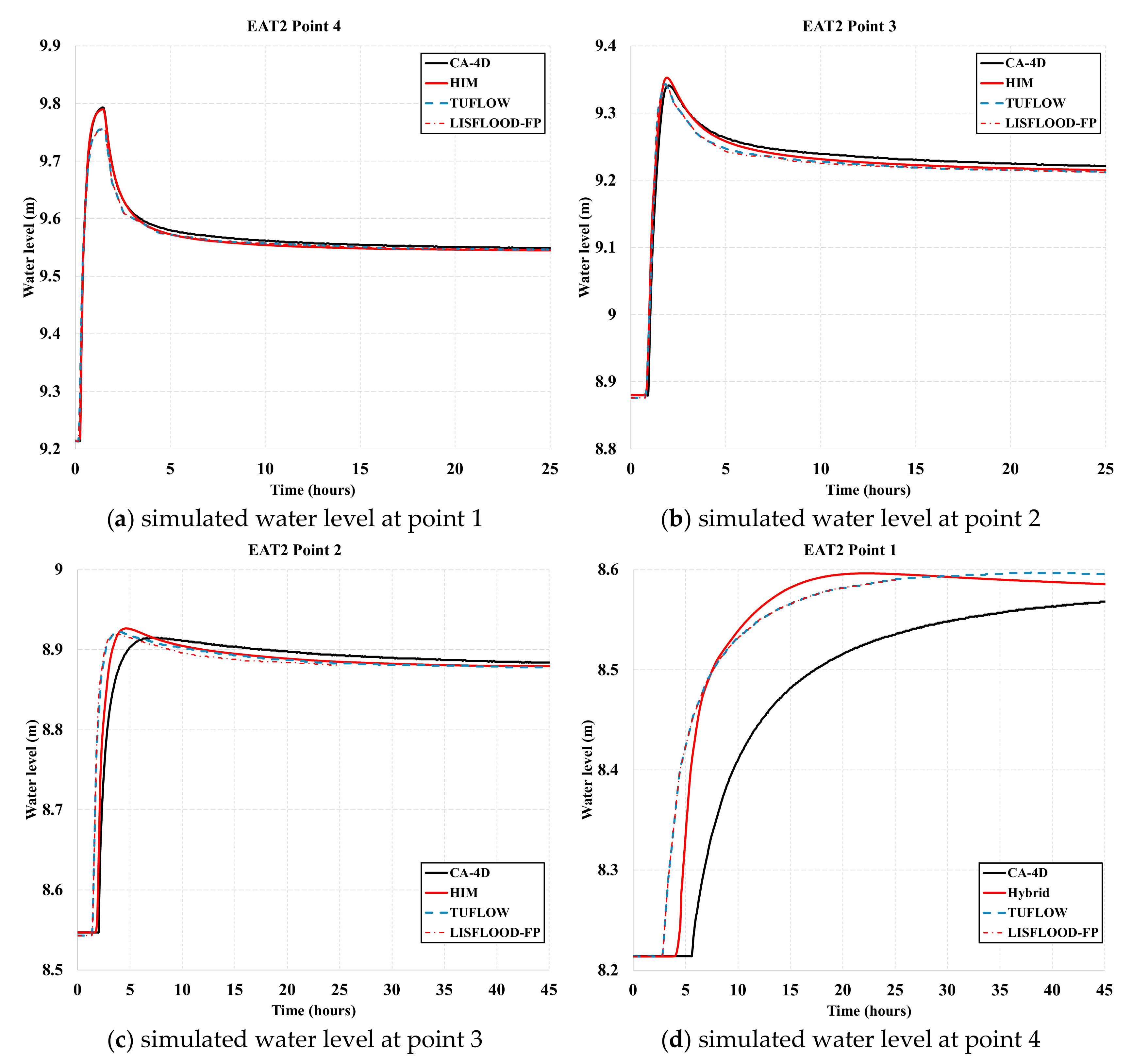
Figure 6 shows a comparison of the water levels at points 1, 2, 3, and 4 for CA-4D, HIM, TUFLOW, and LISFLOOD-FP. The results agree well. However, for the CA-4D result, there is a small discrepancy in water level compared with the TUFLOW and LISFLOOD-FP results, especially at point 1, which is far from the inflow source. The difference in the maximum water levels is 10 cm. At point 1, the CA-4D result slightly lags those of TUFLOW and LISFLOOD-FP in terms of the time when the water begins to fill the depression. This occurs at t = ~3 h in TUFLOW and LISFLOOD-FP and at t = ~6 h in CA-4D. Interestingly, unlike the CA-4D result, the HIM result at point 1 tends to be similar to those of TUFLOW and LISFLOOD-FP.
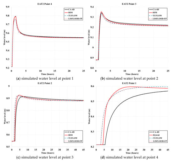
Figure 6.
Temporal variation in the water level for EAT2 at points 1, 2, 3, and 4; comparison among the CA-4D, HIM, TUFLOW, and LISFLOOD-FP models. (a) simulated water level at point 1; (b) simulated water level at point 2; (c) simulated water level at point 3; (d) simulated water level at point 4.
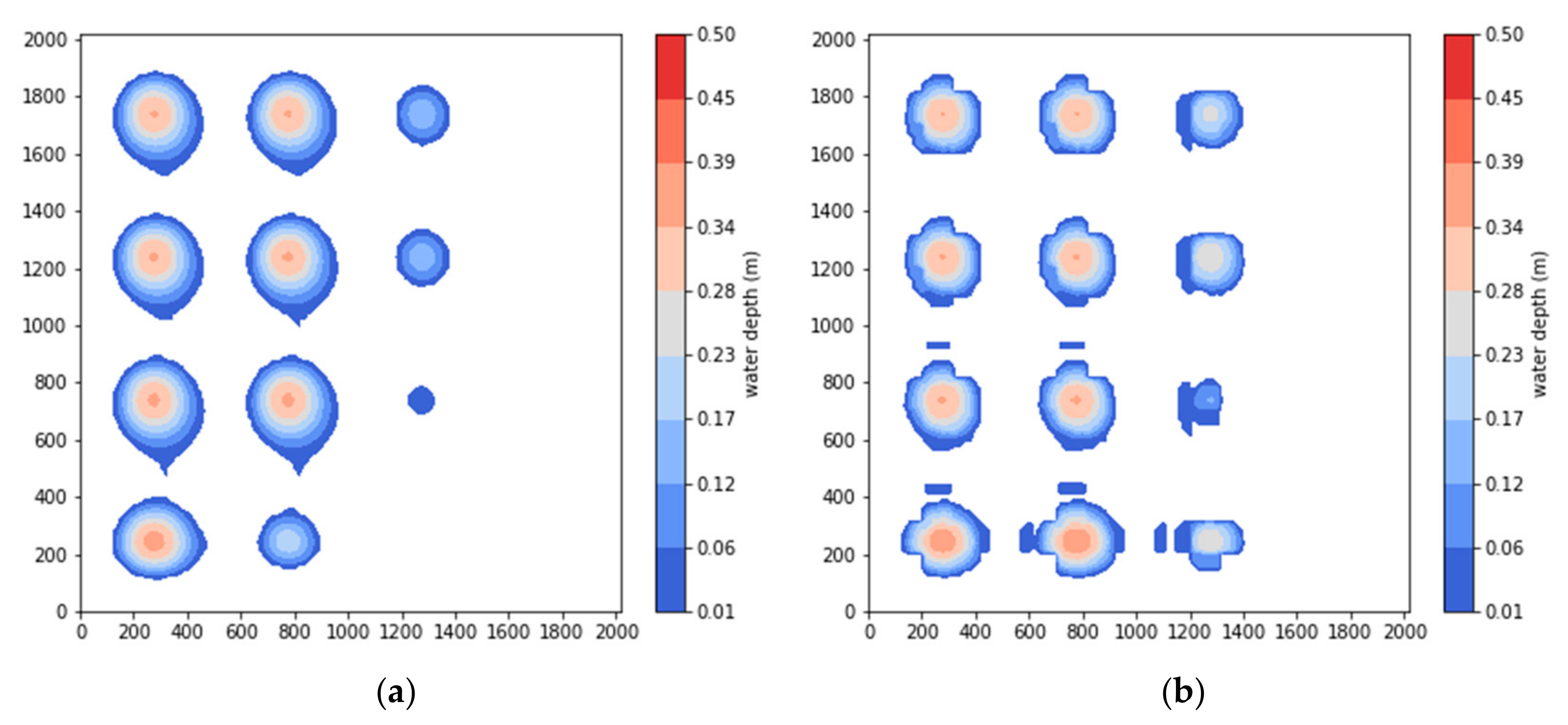
Figure 7 shows a comparison of the flood extent between CA-4D (a) and the HIM (b) at t = 48 h. The HIM shows significant inundation at point 9, while the CA-4D output is completely dry. The discrepancy occurs due to the different grid resolutions that were used. For the HIM, a 100 m grid resolution was used as an input, while for the full CA-4D scenario, a 20 m grid resolution was used. Since the coarse grid resolution data tend to oversimplify the topographic information, the final results of the flood extent might be different. Since there are no observation data, this paper assumes that the flood map produced by CA-4D represents the true value. In this way, the impact of the DEM model can be identified. Based on the performance indicator TPR, the HIM successfully predicts 85% of the area identified by CA-4D as inundated. The FDR shows the percentage of the overpredicted area by the HIM. Based on the calculation, the FDR is 18.32%. The last performance indicator, RMSE, is 0.047 m. The results show that the DEM model does not strongly negatively impact the results.
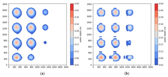
Figure 7.
EAT2: predicted water depth at 48 h by (a) the CA-4D model with 20 m resolution and (b) the HIM.
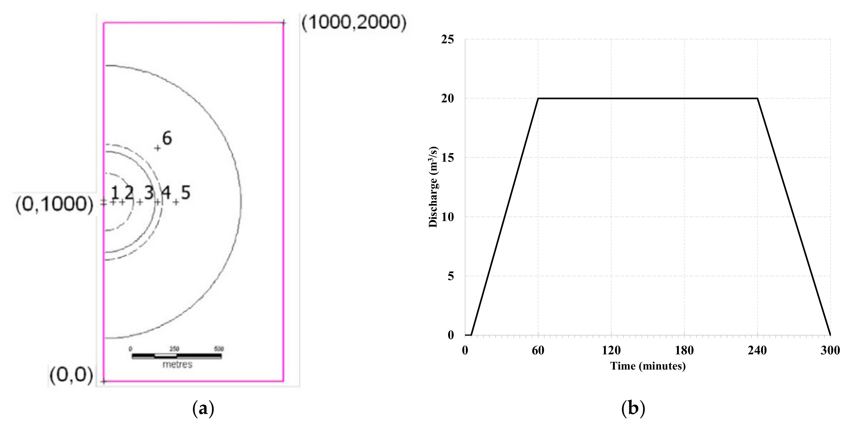
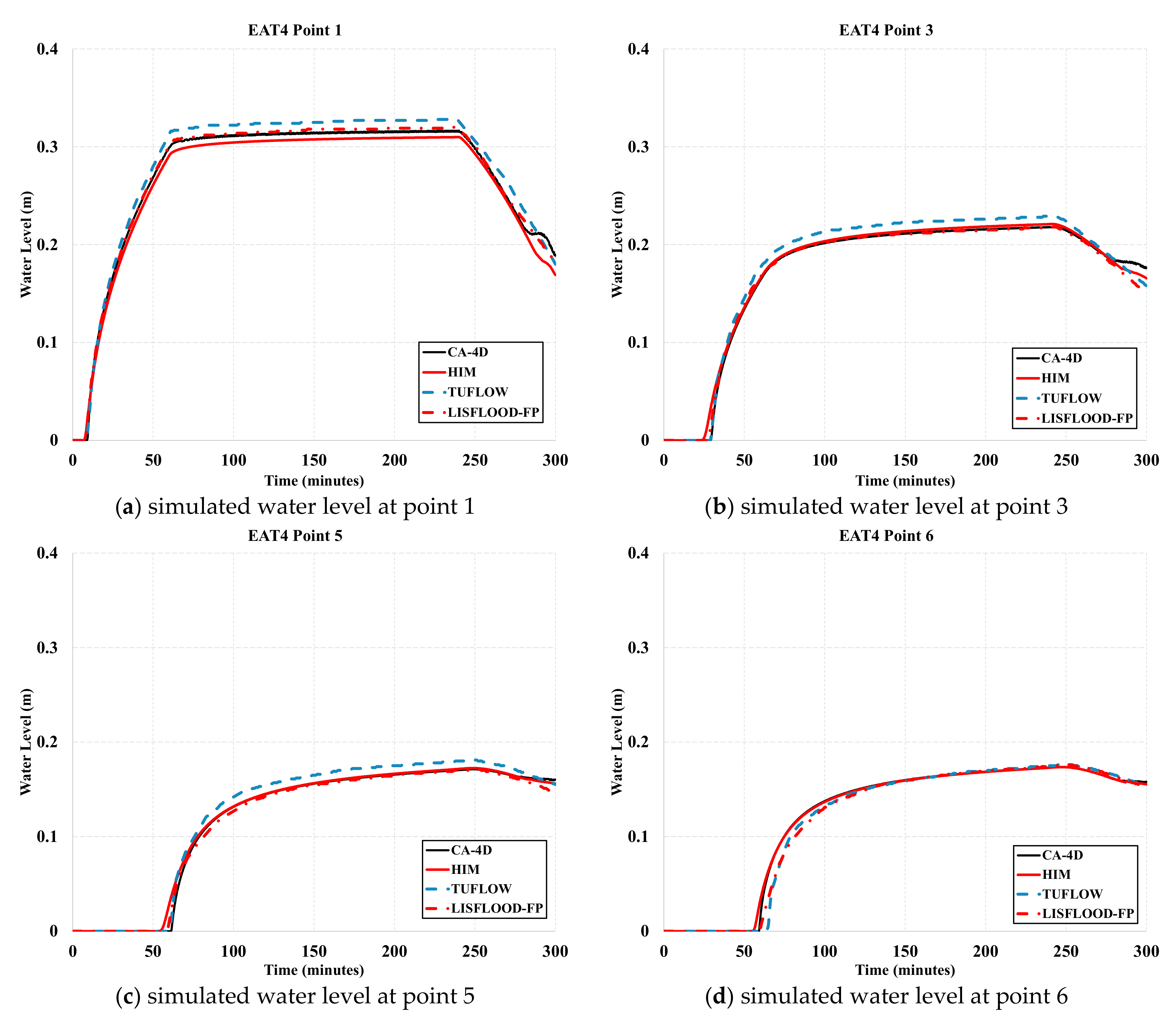
The EAT4 test consisted of a 1000 m × 2000 m horizontal floodplain with a ground elevation of 0 m, and a flood wave occurred due to an overtopping embankment defense failure. The flow boundary condition, as shown in Figure 8b, was applied at the central-west border (x = 0, y = 1000 m). A uniform Manning coefficient of 0.05 m−1/3 s was applied to the whole domain. The scenario was simulated until the time reached 5 h with 6 specified points (see Figure 8a). Figure 9 shows the water level versus time at points 1, 3, 5, and 6. The results obtained from CA-4D and the HIM are in very good agreement with those from TUFLOW and LISFLOOD-FP, with no significant discrepancy. This means that the CA-4D model and HIM show good performance in modeling wave propagation. The HIM successfully predicted 97.7% of the inundated area predicted by CA-4D, and only 0.39% of the area was overpredicted by the HIM. The RMSE value was only 0.0035 m, which is almost negligible.
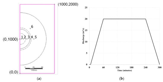
Figure 8.
(a) EAT4 domain with 6 outpoints taken from Néelz and Pender [38] (b) Inflow hydrograph at the central-west point (x, y = 0 m, 1000 m).
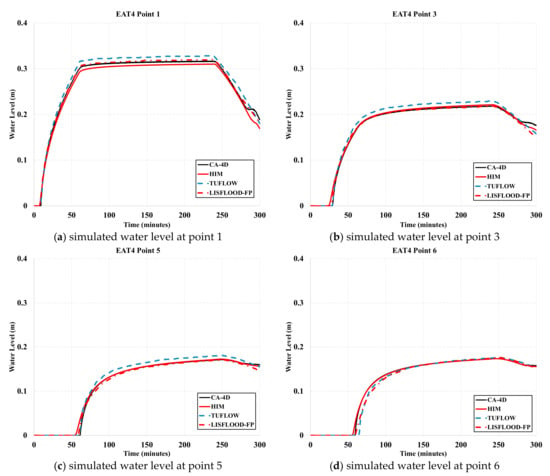
Figure 9.
Temporal variation in water level for EAT4 at points 1, 3, 5, and 6; comparison among the CA-4D, HIM, TUFLOW, and LISFLOOD-FP models; (a) simulated water level at point 1; (b) simulated water level at point 3; (c) simulated water level at point 5; (d) simulated water level at point 6.
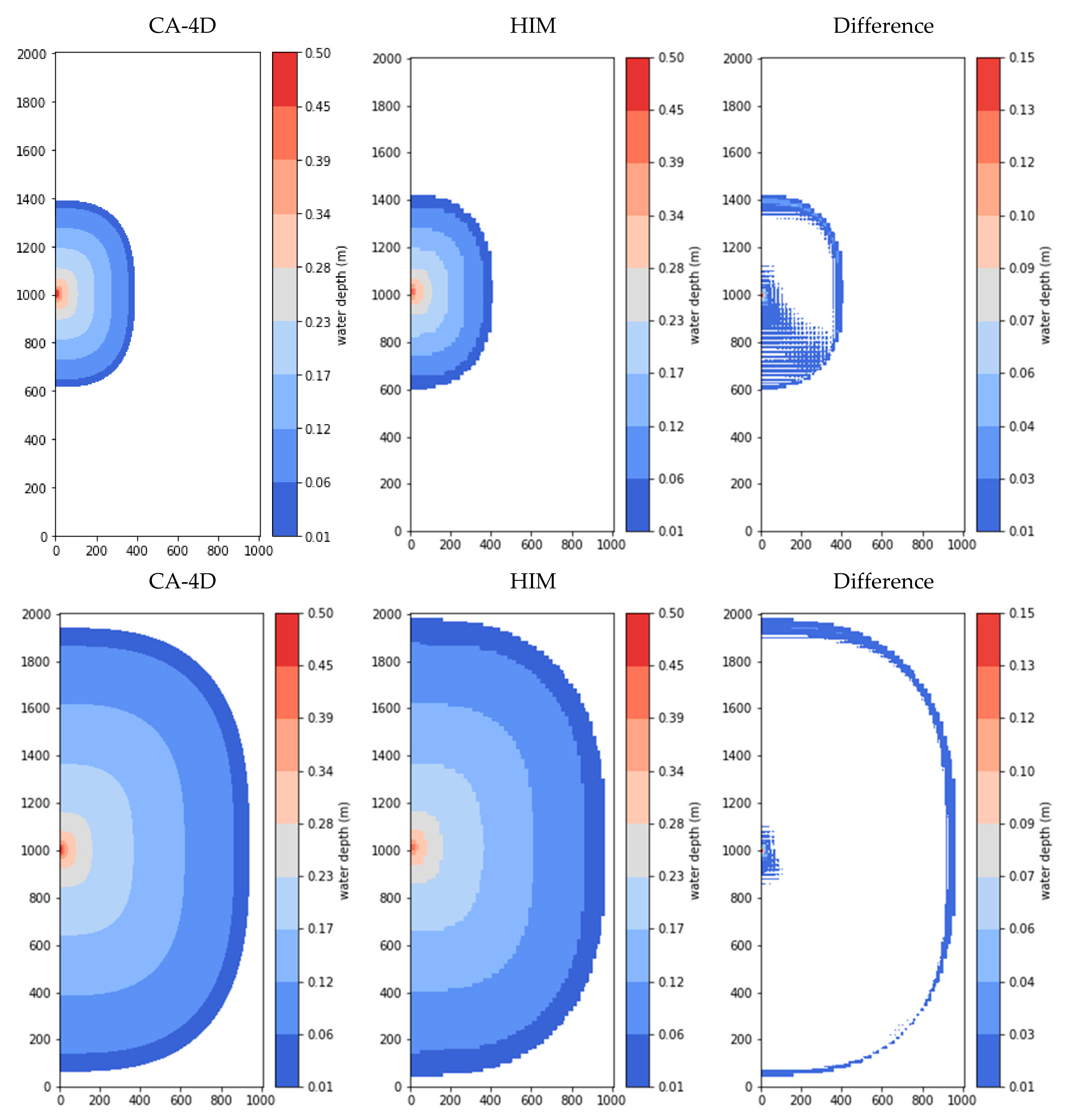
Unlike EAT2 and EAT8A, which involve complex topography, EAT4 involves only flat topography with a 0 m ground elevation. Therefore, the HIM results, which are very sensitive to the grid resolution, do not differ from the other model results. The only difference is the flood extent area. Figure 10 shows that the inundation area produced by the HIM is slightly larger than that of the CA-4D results. As shown in Figure 11, at t = 1 h, the water already propagated at x = 420 m in the HIM and x = 380 m in the CA-4D model. A similar phenomenon was also observed by Hsu et al. [51], who found that the inundation area may increase with coarser DEMs. This makes sense since the HIM model takes the results from the coarse CA-4D as input. However, the difference may be only minimally detectable in flood extent maps.
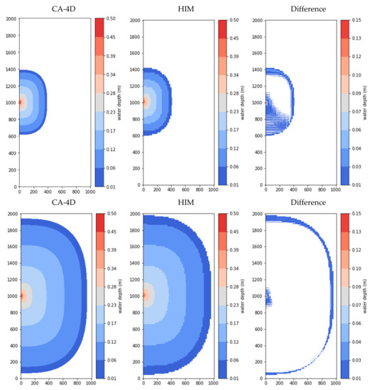
Figure 10.
EAT4: comparison of flood extents at t = 1 h (first row) and at t = 3 h (second row).
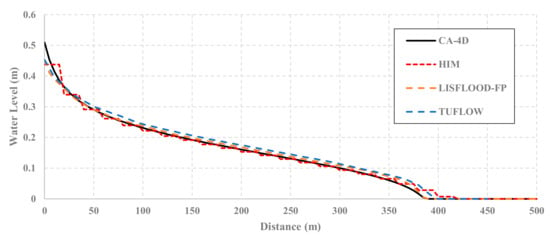
Figure 11.
Cross-section of depths along the line y = 1000 m at t = 1 h.
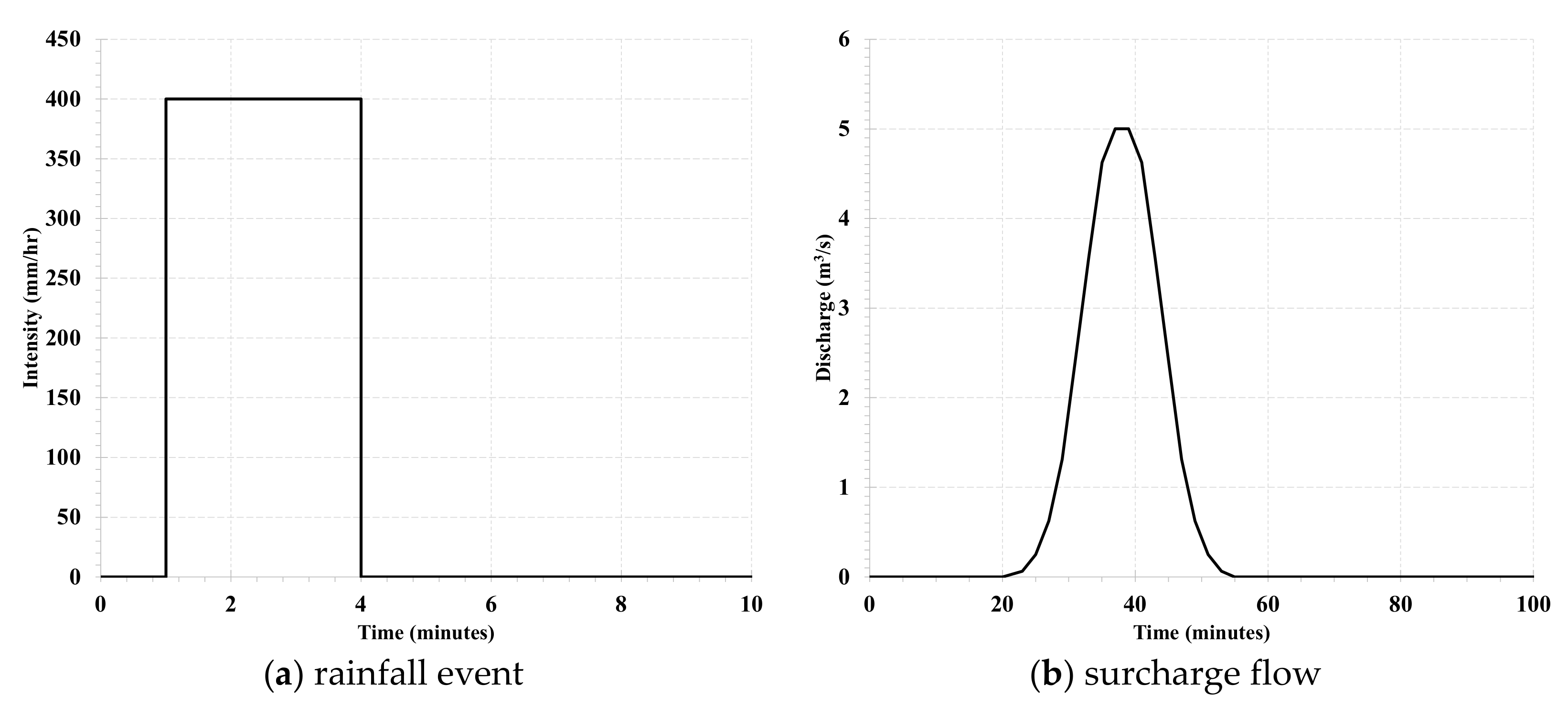
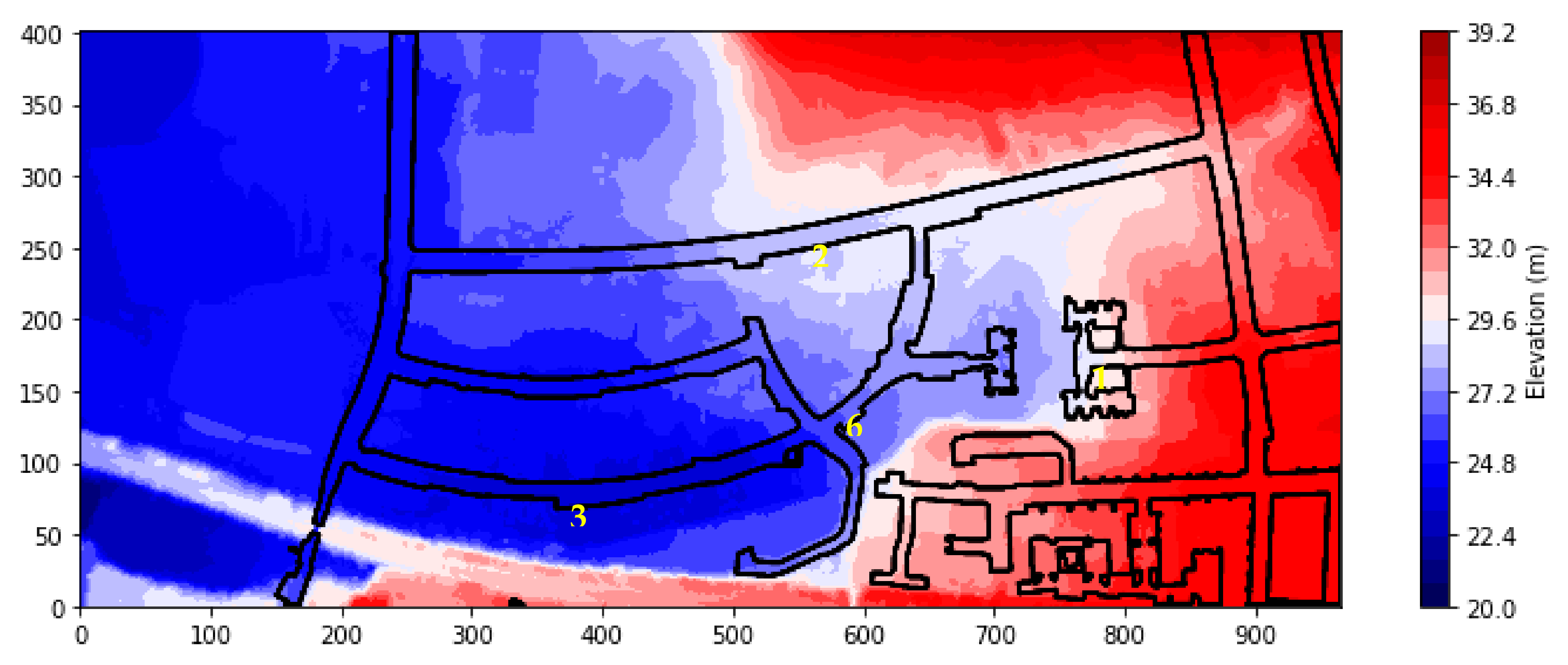
The goal of the EAT8A test is to simulate 2D flood routing within an urban area (Glasgow, UK). The boundary conditions involve two inflow sources: uniform rainfall across the area and surcharge flow located at (x, y = 920 m, 61 m), where the values are given in Figure 12. The study area is approximately 0.4 km2 with an average slope of 4.3%, and the ground elevation ranges from 21 m to 37.6 m. The provided DEM, see Figure 13, is a 0.5 m resolution DEM (no vegetation or buildings) created from LiDAR data. The model is expected to simulate flood routing using a 2 m resolution DEM. Two Manning values are used: 0.02 for road and pavement and 0.05 elsewhere. All boundaries of the domain are closed, and the initial condition is a dry bed.

Figure 12.
EAT8A rainfall event (a) and surcharge flow (b).
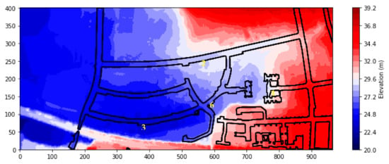
Figure 13.
EAT8A domain in which the area inside the black solid lines is considered the road.
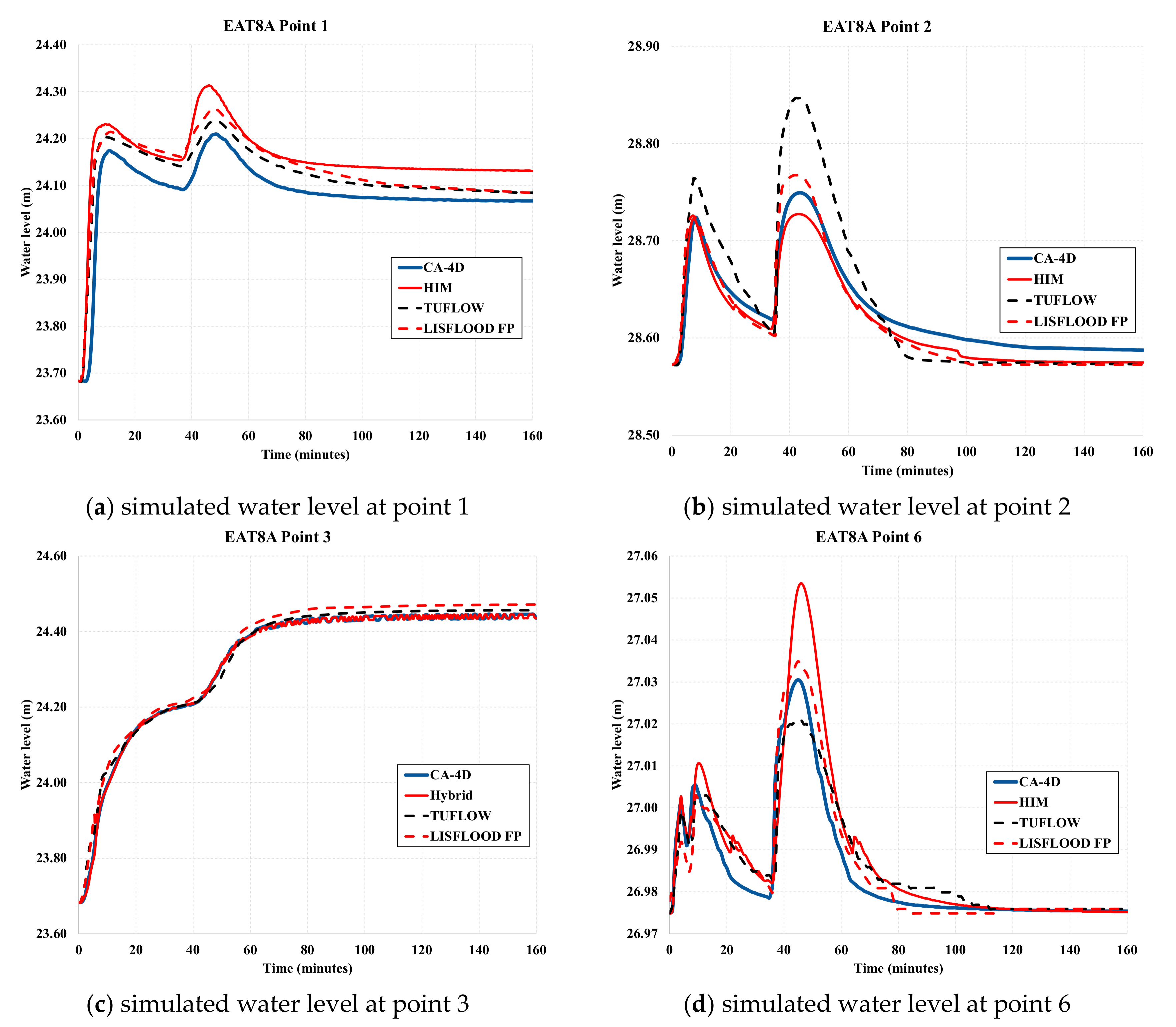
Figure 14 shows that the temporal water levels obtained by CA-4D and the HIM are in good agreement with those of TUFLOW and LISFLOOD-FP. All stage hydrographs show two peaks. This phenomenon is caused by the two inflows coming at different times. Although the results are well correlated, some small discrepancies occur in the HIM and CA-4D results. Some small oscillations in the CA-4D and HIM models at point 3 are visible even though they do not greatly disrupt the overall results. Hunter et al. [15] mentioned that this kind of problem is likely, especially when considering deep water. It could be solved easily by reducing the value of parameter α. However, doing so would dramatically increase the computation time.
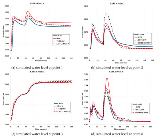
Figure 14.
Temporal variation in water level for EAT8A at points 1, 2, 3, and 6; comparison among the CA-4D, HIM, TUFLOW, and LISFLOOD-FP models; (a) simulated water level at point 1; (b) simulated water level at point 2; (c) simulated water level at point 3; (d) simulated water level at point 6.
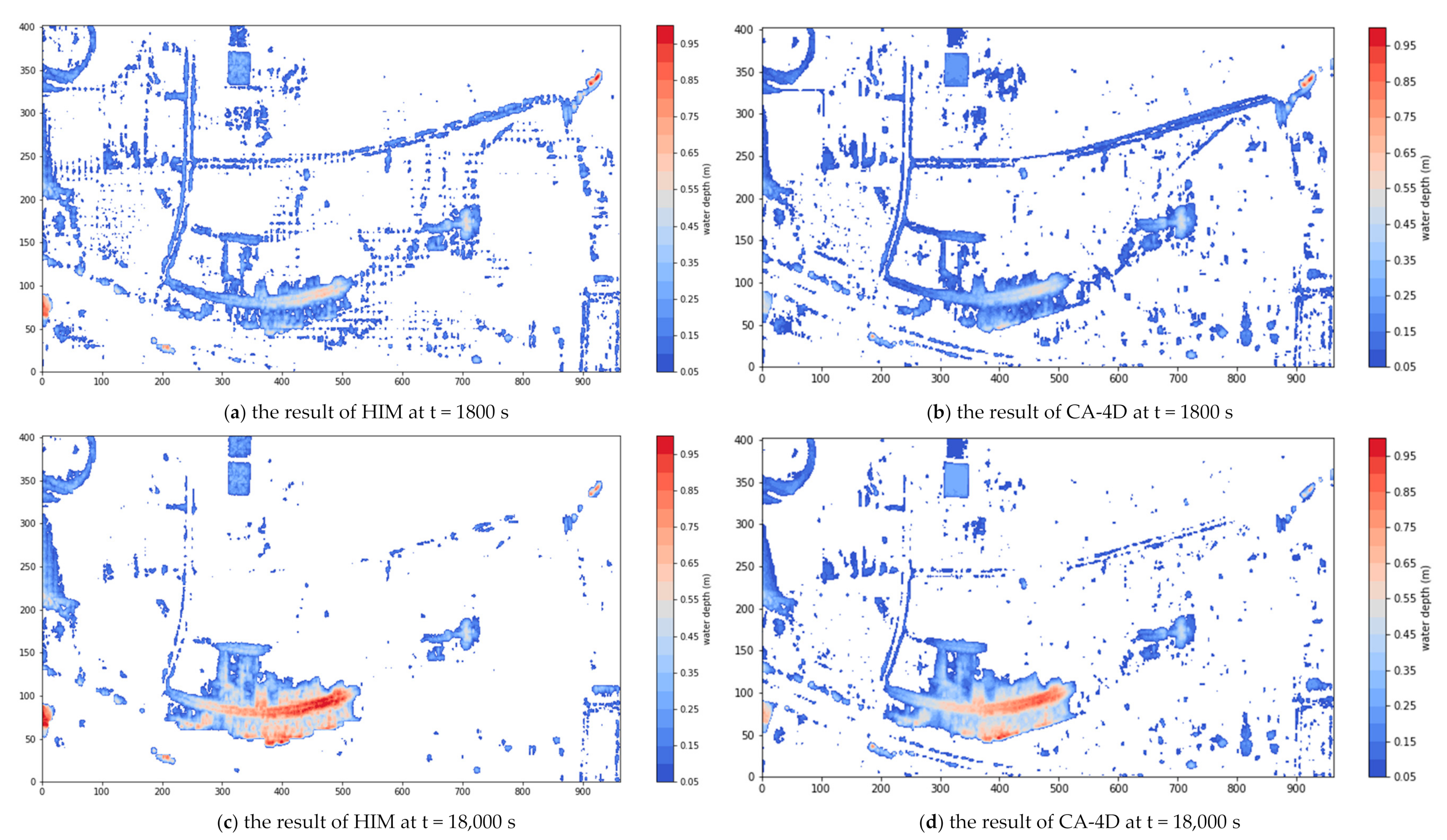
Some differences occurred in the predicted maximum water level. At points 1 and 6, the hybrid simulation predicted values 5–10 cm and 2–3 cm, respectively, higher than the other models’ results. Moreover, at point 2, the hybrid simulation gave the lowest maximum water level compared to the others, especially the TUFLOW result. This primarily occurred because, at point 2, the water movement was primarily driven by momentum. LISFLOOD and CA-4D, which neglect the momentum equation, returned similar results. Figure 15 shows the flood extent predicted by CA-4D and the HIM. Visually, the inundation areas predicted by both models exhibit very good agreement. This conclusion is supported by a TPR value equal to 84.5%, an FDR value equal to 15.6%, and an RMSE value equal to 0.08 m. The results are also in good agreement with those of Jamali et al. [49]. Three models—namely, TUFLOW, HEC-RAS, and CA-ffé—were applied by Jamali et al. [49], and only a slight difference was found in the maximum inundation depth.
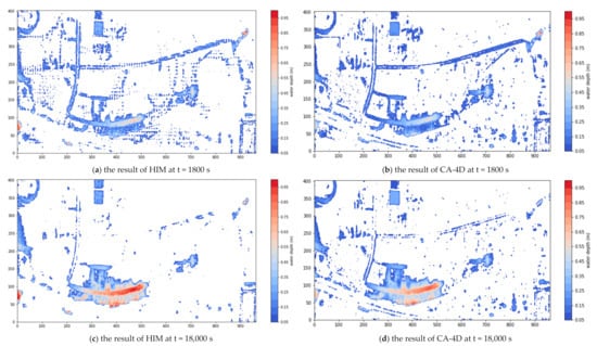
Figure 15.
Flood extents produced by the HIM (left column) and CA-4D (right column) at t = 1800 s (first row) and t = 18,000 s (second row); (a) the result of HIM at t = 1800 s; (b) the result of CA-4D at t = 1800 s; (c) the result of HIM at t = 18,000 s; (d) the result of CA-4D at t = 18,000 s.
4.2. Coastal Areas of Chiayi County
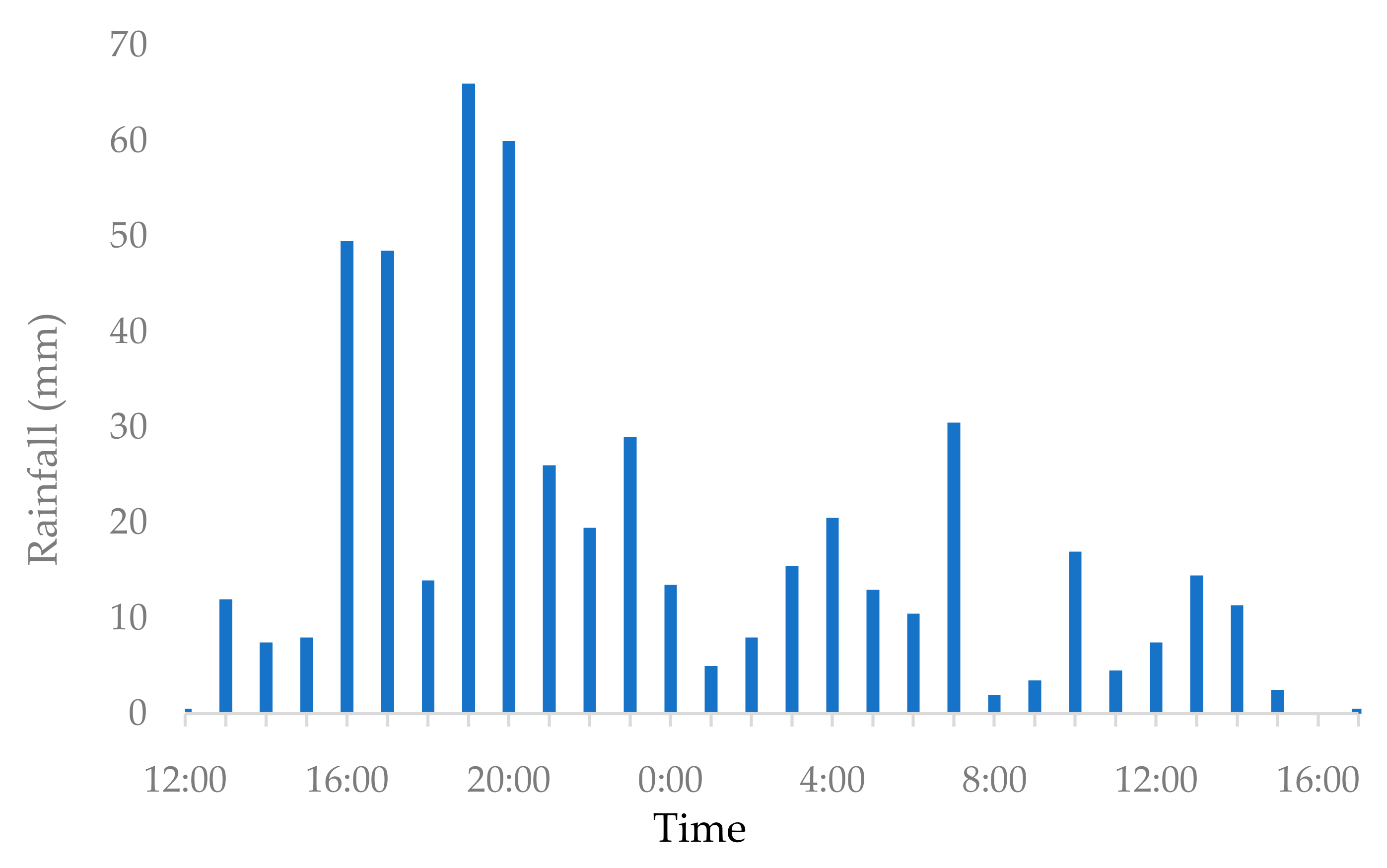
The Chiayi County area is a low-elevation and relatively flat area located near the coastal region. The total area of the simulated domain is approximately 33 km2. A rainfall event of 550 mm over 30 h was applied to the whole domain, and the temporal distribution is shown in Figure 16. The drainage system was not included since this is not yet implemented in the HIM. However, this is reasonable in this case since the drainage system was reported as having failed due to a high tide. The full simulation time was 36 h. To examine the effect of the DEM ratio, two scenarios that used different DEM ratios were simulated. Two coarse DEMs with resolutions of 25 and 40 m, obtained from averaging the 5 m DEM, were used as an input for the CA-4D model, and within this study, these are called the C25 m and C40 m scenarios, respectively. The D-Flat model interpolated the outputs from CA-4D into 5 m resolution results.

Figure 16.
Rainfall distribution in Chiayi County on 23–24 August 2018.
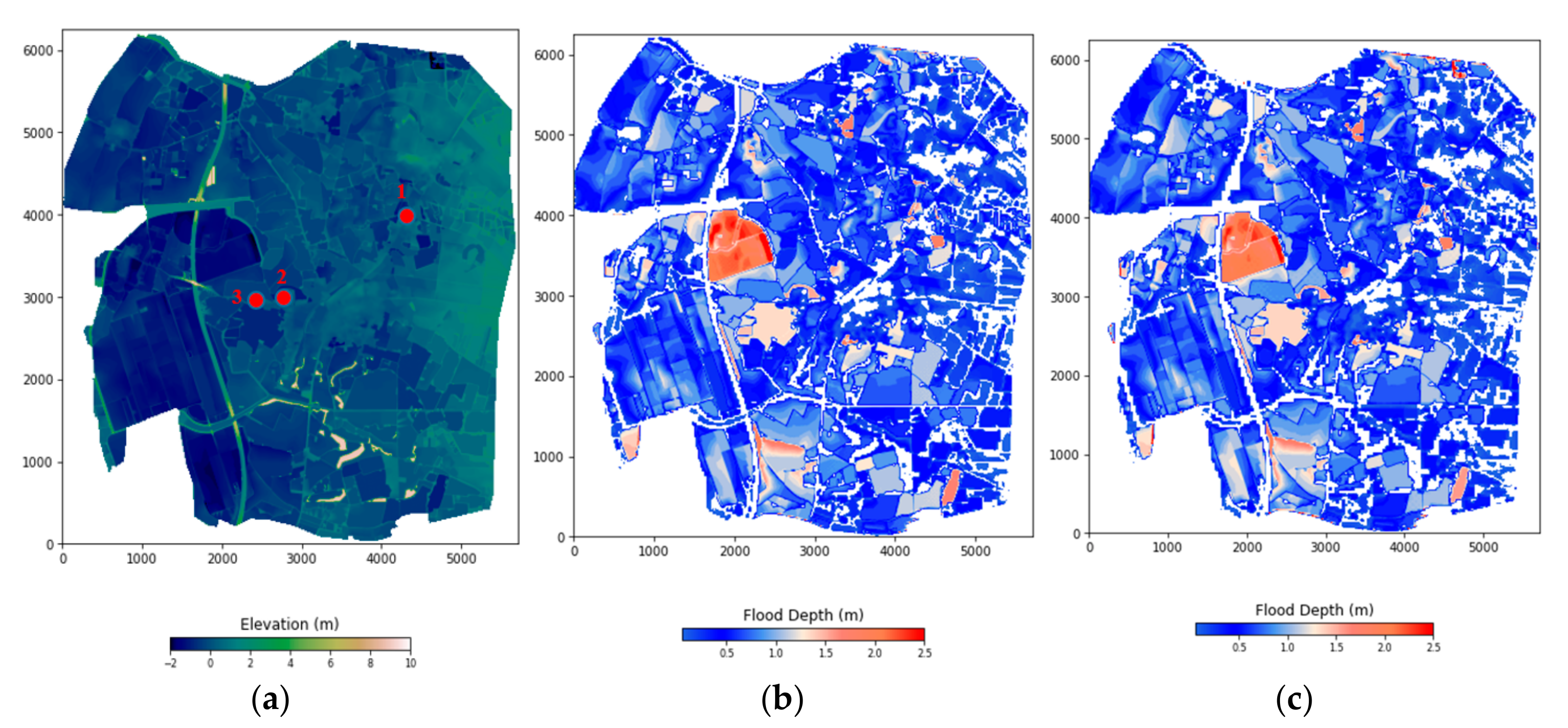
Figure 17 shows the DEM of the area with the observation points, indicated by the red dots, and the maximum flood extent predicted by both DEM ratios. The water flows from east to west due to topography. Two detention ponds are located on the left-hand side of the map. The DEM ratio has a significant impact on the model performance. Figure 17a,c show that the two ratios produce almost identical maximum flood extents. Floodwater accumulates in particular on the left-hand side of the map, and some differences are found in the areas near the boundaries. This study area is similar to the ET4 case, in which the area is topographically flat. The result shows that the impact of the DEM ratio is small when the study area is flat. Hence, this allows for a higher DEM ratio to be used. In this case, the DEM ratio of C25m is 5, while that of C40 m is 8.
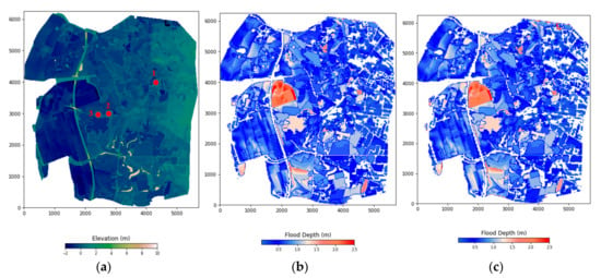
Figure 17.
Maximum flood extent of the (a) Chiayi County DEM and observation points (red dots), (b) C25 m and (c) C40 m.
The maximum flood depths were collected at three different locations, as shown in Figure 17a. It is known that the observations are not from gaging stations but local surveys. Table 2 shows the comparisons between the observation data and the simulation results. The observations showed that the locations of points 1 and 2 were inundated, and point 3 was not. The HIM results are consistent with this finding. Overall, there is no significant difference between the C25 m and C40 m results. However, compared to the observation data, there is a 50% difference at point 2. This study used TUFLOW to simulate the study area and used the results to verify the HIM performance. The HIM and TUFLOW results are compared with observations in Table 2. The difference is less than 10 cm in all observations. The results confirm the flood prediction capability of the HIM.

Table 2.
Comparison of observed and simulated maximum flood depths at different locations.
4.3. Model Efficiency
All simulations were run using an Intel Core i7-8550U CPU @ 1.80 GHz without parallel or graphics processing unit computations. Table 3 shows the computation times for the three EA benchmark case simulations and coastal areas of the Chiayi County case. When compared to the TUFLOW and LISFLOOD-FP computation times, for the EA benchmark cases, the CA-4D and HIM computation times were longer for all simulations. This is attributed to TUFLOW and LISFLOOD-FP using massive parallelism to accelerate computation. However, the HIM shows a significantly shorter computation time than CA-4D: 30 and 35 times faster to obtain the EAT2 and EAT4 results, respectively. The EAT8A results show that the CA-4D computation time was massive: more than 2 weeks to finish the 5-h simulation. This massive computation time was caused by the very fine resolution being used (2 m). As a consequence, the time step decreased to ensure model stability. The HIM did not face this kind of problem since a coarse grid resolution was used (10 m). That is, the HIM could finish the simulation up to 1200 times faster. These results show that the hybrid process could enhance the efficiency of the CA-4D model without using any parallelism technique. From the real case study, it could be seen that the HIM computation time could be decreased even more by simply increasing the DEM ratio. Scenario C25m, which used a ratio of 5, produced a computation time similar to that of TUFLOW-GPU. However, scenario C40m, which used a ratio of 8, was almost 7 times faster than TUFLOW-GPU. However, the DEM ratio cannot be increased carelessly since a higher DEM ratio returns less accurate results.

Table 3.
Comparison of the computation times.
5. Conclusions
The rapid flood model HIM is presented in this study, and the performance was evaluated using three case studies from the EA-UK benchmark tests and a historical event in a coastal area in Chiayi County. The stage hydrographs produced by the HIM for the three UK EA test cases (EAT2, EAT4, and EAT8A) at various points are consistent with those of the commercial software TUFLOW and LISFLOOD-FP. To evaluate the performance of the combination, the results of a purely CA model (CA-4D) and the HIM were compared. Some discrepancies occurred between the flood extent predicted by CA-4D and the HIM in EAT2 because the HIM is very sensitive to the grid resolution. However, the inundation extents predicted by both models show very good agreement for all cases. Based on these three cases from EA-UK, the performance indexes of the TPR and FDR range from 85–97% and from 0.39–18%, respectively, and the RMSEs are between 0.047 m and 0.08 m. In terms of efficiency, the computation time of the HIM compared to that of CA-4D shows that the HIM was 23 to 1200 times faster. It can be concluded that the HIM can provide faster results than a CA-based flood model without significantly sacrificing accuracy.
Finally, a historical flood event was also investigated in this study, and two grid combination scenarios, C25m and C40m, were conducted to determine the effect of the DEM ratio on the results. The performance was also confirmed when the simulated results were compared with the TUFLOW model. The computation time could be reduced by simply increasing the DEM ratio. However, by doing so, the model must sacrifice the accuracy of the result. Therefore, further study on the optimal DEM ratio must be performed in the future so that the results of the HIM can meet the needs of emergency response. Compared to the observation data, the grid ratios showed no difference, and all results underpredicted the flood depth at some points. One reason is that the simplified governing equations in HIM may not provide enough accuracy. Since the flood record was collected based on the local surveys, its accuracy may be also be an issue. Overall, the concept of combining CA and DEM models shows potential for practical purposes. However, certain components, such as drainage systems and detention basins, which are common in urban areas, are not included in the HIM model. Further research must be conducted to include these features to increase the accuracy of simulations in urban areas. The DEM ratio between CA-4D and D-Flat in the HIM is not investigated in this study. It is expected to have a nonlinear impact on the results. The best DEM ratio is therefore a topic to be further investigated in the future. The results have shown the model’s potential, and considerable work remains for the model to be capable of meeting the requirements of real applications. Furthermore, the governing equations considered in the HIM are simplified. They can provide only a certain degree of accuracy when attempting to meet the needs of emergency response. In conclusion, the HIM is not the model that should be selected for detailed simulations or situations that demand high standards of accuracy.
Author Contributions
O.T.W. and T.-H.Y. developed the theoretical formalism, performed the analytic calculations and performed the numerical simulations. Both O.T.W. and T.-H.Y. contributed to the final version of the manuscript. All authors have read and agreed to the published version of the manuscript.
Funding
This study was supported by the Ministry of Science and Technology of Taiwan under Research Grant MOST 109-2625-M-009-006. The authors have no conflicts of interest to declare.
Informed Consent Statement
Informed consent was obtained from all subjects involved in the study.
Data Availability Statement
The data that support the findings of this study are available from the corresponding author, T.-H.Y., upon reasonable request.
Acknowledgments
The authors would like to thank the UK Environment Agency for the EA benchmark datasets and National Science and Technology Center for Disaster Reduction for the observation records.
Conflicts of Interest
The authors have no conflict of interest to declare.
References
- Mizutori, M.; Guha-Sapir, D. Economic Losses, Poverty and Disasters 1998–2017; United Nations Office for Disaster Risk Reduction: Geneva, Switzerland, 2017. [Google Scholar] [CrossRef]
- Luo, T.; Maddocks, A.; Iceland, C.; Ward, P.; Winsemius, H. World’s 15 Countries with the Most People Exposed to River Floods. Available online: http://www.wri.org/blog/2015/03/world%E2%80%99s-15-countries-most-people-exposed-river-floods (accessed on 16 March 2021).
- Albano, R.; Sole, A.; Adamowski, J.; Mancusi, L. A GIS-based model to estimate flood consequences and the degree of accessibility and operability of strategic emergency response structures in urban areas. Nat. Hazards Earth Syst. Sci. 2014, 14, 2847–2865. [Google Scholar] [CrossRef]
- Galland, J.C.; Goutal, N.; Hervouet, J.M. TELEMAC: A new numerical model for solving shallow water equations. Adv. Water Resour. 1991, 14, 138–148. [Google Scholar] [CrossRef]
- Innovyze. InfoWorks ICM Help v3.0. Available online: https://help.innovyze.com/display/infoworksicm/InfoWorks+ICM+Help+Documentation (accessed on 16 March 2021).
- DHI Software. MIKE FLOOD. Available online: https://www.mikepoweredbydhi.com/products/mike-flood (accessed on 7 June 2019).
- Henonin, J.; Russo, B.; Mark, O.; Gourbesville, P. Real-time urban flood forecasting and modelling—A state of the art. J. Hydroinform. 2013, 15, 717–736. [Google Scholar] [CrossRef]
- Lavoie, B.; Mahdi, T.F. Comparison of two-dimensional flood propagation models: SRH-2D and HYDRO_AS-2D. Nat. Hazards 2017, 86, 1207–1222. [Google Scholar] [CrossRef]
- Ginting, B.M.; Mundani, R.P. Parallel flood simulations for wet–dry problems using dynamic load balancing concept. J. Comput. Civ. Eng. 2019, 33, 04019013. [Google Scholar] [CrossRef]
- Huxley, C.; Syme, B. TUFLOW GPU-best practice advice for hydrologic and hydraulic model simulations. In Proceedings of the 37th Hydrology & Water Resources Symposium 2016: Water, Infrastructure and the Environment, Queenstown, New Zealand, 28 November–2 December 2016; Engineers Australia: Queenstown, New Zealand, 2016; p. 195. [Google Scholar]
- Lamb, R.; Crossley, M.; Waller, S. A fast two-dimensional floodplain inundation model. Proc. Inst. Civ. Eng. Water Manag. 2009, 162, 363–370. [Google Scholar] [CrossRef]
- Guidolin, M.; Chen, A.S.; Ghimire, B.; Keedwell, E.C.; Djordjević, S.; Savić, D.A. A weighted cellular automata 2D inundation model for rapid flood analysis. Environ. Model. Softw. 2016, 84, 378–394. [Google Scholar] [CrossRef]
- Bates, P.D.; Horritt, M.S.; Fewtrell, T.J. A simple inertial formulation of the shallow water equations for efficient two-dimensional flood inundation modelling. J. Hydrol. 2010, 387, 33–45. [Google Scholar] [CrossRef]
- Bates, P.D.; De Roo, A.P.J. A simple raster-based model for flood inundation simulation. J. Hydrol. 2000, 236, 54–77. [Google Scholar] [CrossRef]
- Hunter, N.M.; Horritt, M.S.; Bates, P.D.; Wilson, M.D.; Werner, M.G.F. An adaptive time step solution for raster-based storage cell modelling of floodplain inundation. Adv. Water Resour. 2005, 28, 975–991. [Google Scholar] [CrossRef]
- Bradbrook, K.F.; Lane, S.N.; Waller, S.G.; Bates, P.D. Two dimensional diffusion wave modelling of flood inundation using a simplified channel representation. Int. J. River Basin Manag. 2004, 2, 211–223. [Google Scholar] [CrossRef]
- Chen, A.; Djordjević, S.; Leandro, J.; Savic, D. The urban inundation model with bidirectional flow interaction between 2D overland surface and 1D sewer networks. In Proceeding of the 6th NOVATECH International Conference, Lyon, Rhone-Alpes, France, 25–28 June 2007; Workshop I Graie: Lyon, France, 2007; pp. 465–472. [Google Scholar]
- Fewtrell, T.J.; Bates, P.D.; Horritt, M.; Hunter, N.M. Evaluating the effect of scale in flood inundation modelling in urban environments. Hydrol. Process. 2008, 22, 5107–5118. [Google Scholar] [CrossRef]
- Glenis, V.; McGough, A.S.; Kutija, V.; Kilsby, C.; Woodman, S. Flood modelling for cities using cloud computing. J. Cloud Comput. Adv. Syst. Appl. 2013, 2, 7. [Google Scholar] [CrossRef]
- Caviedes-Voullième, D.; Fernández-Pato, J.; Hinz, C. Cellular automata and finite volume solvers converge for 2D shallow flow modelling for hydrological modelling. J. Hydrol. 2018, 563, 411–417. [Google Scholar] [CrossRef]
- Wolfram, S. Cellular automata as models of complexity. Nature 1984, 311, 419–424. [Google Scholar] [CrossRef]
- Blecic, I.; Cecchini, A.; Prastacos, P.; Trunfio, G.; Verigos, E. Modelling urban dynamics with cellular automata: A model of the city of Heraclion. In Proceedings of the 7th AGILE Conference on Geographic Information Science, Heraklion, Greece, 29 April–1 May 2004; University of Crete Press: Heraklion, Greece, 2004. [Google Scholar]
- Pérez-Molina, E.; Sliuzas, R.; Flacke, J.; Jetten, V. Developing a cellular automata model of urban growth to inform spatial policy for flood mitigation: A case study in Kampala, Uganda. Comput. Environ. Urban Syst. 2017, 65, 53–65. [Google Scholar] [CrossRef]
- Freire, J.G.; DaCamara, C.C. Using cellular automata to simulate wildfire propagation and to assist in fire management. Nat. Hazards Earth Syst. Sci. 2018, 19, 169–179. [Google Scholar] [CrossRef]
- D’Ambrosio, D.; Di Gregorio, S.; Iovine, G. Simulating debris flows through a hexagonal cellular automata model: SCIDDICA S3–hex. Nat. Hazards Earth Syst. Sci. 2003, 3, 545–559. [Google Scholar] [CrossRef]
- Iovine, G.; Di Gregorio, S.; Lupiano, V. Debris-flow susceptibility assessment through cellular automata modeling: An example from 15–16 December 1999 disaster at Cervinara and San Martino Valle Caudina (Campania, Southern Italy). Nat. Hazards Earth Syst. Sci. 2003, 3, 457–468. [Google Scholar] [CrossRef]
- Lupiano, V.; Chidichimo, F.; Machado, G.; Catelan, P.; Molina, L.; Calidonna, C.R.; Straface, S.; Crisci, G.M.; Di Gregorio, S. From examination of natural events to a proposal for risk mitigation of lahars by a cellular-automata methodology: A case study for Vascún valley, Ecuador. Nat. Hazards Earth Syst. Sci. 2020, 20, 1–20. [Google Scholar] [CrossRef]
- Aljoufie, M.; Zuidgeest, M.; Brussel, M.; van Vliet, J.; van Maarseveen, M. A cellular automata-based land use and transport interaction model applied to Jeddah, Saudi Arabia. Landsc. Urban Plan. 2013, 112, 89–99. [Google Scholar] [CrossRef]
- Dottori, F.; Todini, E. A 2D flood inundation model based on cellular automata approach. In Proceedings of the XVIII International Conference on Water Resources, Barcelona, Spain, 21–24 June 2010; Carrera, J., Ed.; CMWR: Barcelona, Spain, 2010. [Google Scholar]
- Dottori, F.; Todini, E. Developments of a flood inundation model based on the cellular automata approach: Testing different methods to improve model performance. Phys. Chem. Earth Parts A/B/C 2011, 36, 266–280. [Google Scholar] [CrossRef]
- Ghimire, B.; Chen, A.S.; Guidolin, M.; Keedwell, E.C.; Djordjević, S.; Savić, D.A. Formulation of a fast 2D urban pluvial flood model using a cellular automata approach. J. Hydroinform. 2013, 15, 676–686. [Google Scholar] [CrossRef]
- Liu, L.; Liu, Y.; Wang, X.; Yu, D.; Liu, K.; Huang, H.; Hu, G. Developing an effective 2-D urban flood inundation model for city emergency management based on cellular automata. Nat. Hazards Earth Syst. Sci. 2015, 15, 381–391. [Google Scholar] [CrossRef]
- Wijaya, O.T.; Yang, T.H. Combining two algorithms as a transition rules for CA-based inundation model. In Proceedings of the 22nd IAHR APD, Saporo, Japan, 15–16 September 2020. [Google Scholar]
- Issermann, M.; Chang, F.J.; Jia, H. Efficient urban inundation model for live flood forecasting with cellular automata and motion cost fields. Water 2020, 12, 1997. [Google Scholar] [CrossRef]
- Topa, P.; Młocek, P. GPGPU implementation of cellular automata model of water flow. In Proceedings of the International Conference on Parallel Processing and Applied Mathematics, Torun, Poland, 11–14 September 2011. [Google Scholar]
- Chen, J.; Hill, A.A.; Urbano, L.D. A GIS-based model for urban flood inundation. J. Hydrol. 2009, 373, 184–192. [Google Scholar] [CrossRef]
- CH2M. ISIS FAST. Available online: http://help.floodmodeller.com/isis/ISIS_Fast.htm (accessed on 16 March 2021).
- Yang, T.H.; Chen, Y.C.; Chang, Y.C.; Yang, S.C.; Ho, J.Y. Comparison of different grid cell ordering approaches in a simplified inundation model. Water 2015, 7, 438–454. [Google Scholar] [CrossRef]
- Jamali, B.; Löwe, R.; Bach, P.M.; Urich, C.; Arnbjerg-Nielsen, K.; Deletic, A. A rapid urban flood inundation and damage assessment model. J. Hydrol. 2018, 564, 1085–1098. [Google Scholar] [CrossRef]
- Garcia-Navarro, P. Advances in numerical modelling of hydrodynamics workshop, university of Sheffield, UK, March 24–25, 2015. Appl. Math. Model. 2016, 40, 7423. [Google Scholar] [CrossRef]
- Bates, P.D. Development and testing of a subgrid-scale model for moving boundary hydrodynamic problems in shallow water. Hydrol. Process. 2000, 14, 2073–2088. [Google Scholar] [CrossRef]
- Sanders, B.F.; Schubers, J.E. PRIMo: Parallel raster inundation model. Adv. Water Resour. 2019, 126, 79–95. [Google Scholar] [CrossRef]
- Casulli, V.; Stelling, G.S. Semi-implicit subgrid modelling of three-dimensional free-surface flows. Int. J. Numer. Meth. Fluids. 2010, 67, 441–449. [Google Scholar] [CrossRef]
- Jan, A.; Coon, E.T.; Graham, J.D.; Painter, S.L. A subgrid approach for modelling microtopography effects on overland flow. Water Resour. Res. 2018, 54, 6153–6167. [Google Scholar] [CrossRef]
- Keesstra, S.; Nunes, J.P.; Saco, P.; Parsons, T.; Poeppl, R.; Masselink, R.; Cerdà, A. The way forward: Can connectivity be useful to design better measuring and modelling schemes for water and sediment dynamics? Sci. Total Environ. 2018, 644, 1557–1572. [Google Scholar] [CrossRef]
- Cerdà, A.; Novara, A.; Dlapa, P.; López-Vicente, M.; Úbeda, X.; Popović, Z.; Mekonnen, M.; Terol, E.; Janizadeh, S.; Mbarki, S.; et al. Rainfall and water yield in Macizo del Caroig, Eastern Iberian Peninsula. Event runoff at plot scale during a rare flash flood at the Barranco de Benacancil. Cuad. Investig. Geogr. 2021. [Google Scholar] [CrossRef]
- Néelz, S.; Pender, G. Benchmarking the Latest Generation of 2D Hydraulic Modelling Packages; UK Environment Agency: Rotherham, UK, 2013. [Google Scholar]
- Shen, Y.; Morsy, M.M.; Huxley, C.; Tahvildari, N.; Goodall, J.L. Flood risk assessment and increased resilience for coastal urban watersheds under the combined impact of storm tide and heavy rainfall. J. Hydrol. 2019, 579, 124159. [Google Scholar] [CrossRef]
- Jamali, B.; Bach, P.M.; Cunningham, L.; Deletic, A. A cellular automata fast flood evaluation (CA-ffé) model. Water Resour. Res. 2019, 55, 4936–4953. [Google Scholar] [CrossRef]
- Bennett, N.D.; Croke, B.F.W.; Guariso, G.; Guillaume, J.H.A.; Hamilton, S.H.; Jakeman, A.J.; Marsili-Libelli, S.; Newham, L.T.H.; Norton, J.P.; Perrin, C.; et al. Characterising performance of environmental models. Environ. Model. Softw. 2013, 40, 1–20. [Google Scholar] [CrossRef]
- Hsu, Y.C.; Prinsen, G.; Bouaziz, L.; Lin, Y.J.; Dahm, R. An investigation of DEM resolution influence on flood inundation simulation. Procedia Eng. 2016, 154, 826–834. [Google Scholar] [CrossRef]
Publisher’s Note: MDPI stays neutral with regard to jurisdictional claims in published maps and institutional affiliations. |
© 2021 by the authors. Licensee MDPI, Basel, Switzerland. This article is an open access article distributed under the terms and conditions of the Creative Commons Attribution (CC BY) license (https://creativecommons.org/licenses/by/4.0/).

