Modeling Chlorophyll a with Use of the SWAT Tool for the Nielba River (West-Central Poland) as an Example of an Unmonitored Watercourse

Abstract

The majority of eutrophication studies focuses on lacustrine processes, thus riverine systems remain less recognized in this context. Moreover, since the availability of data related to parameters affecting this phenomenon is quite limited, modeling efforts should be considered. The current study verifies the SWAT model’s capability to simulate chlorophyll a loads for unmonitored watercourse. The analyses of the relationships between individual parameters, directly involved in the eutrophication process, help in the exploration of its dominant trends in SWAT modeling. The results obtained for the Nielba River pilot catchment (west-central Poland) showed a strong correlation of chlorophyll a with flow and surface runoff, but no relationship with temperature or solar radiation. Moreover, an impact of local conditions (hydrological features) on chlorophyll a load simulation could be traced in detail. The research specified the limitations and impact of generalization in the SWAT model on the results. Furthermore, intricacies related to the dataset statistical treatment (e.g., outliers) have been presented.

1. Introduction

The eutrophication phenomenon has been studied for many years [1,2,3,4,5,6,7,8,9,10]. Currently, it is defined as not a “state,” but a “process” which requires action of external factors to bring changes into a system. These changes, result from enrichment of waters in nutrients and stimulation of organic matter production. Under favorable conditions, such as light access, proper temperatures, and a suitable ratio of nitrogen and phosphorus in water, eutrophication leads to the excessive growth of phytoplankton and vegetation. Excessive growth of algae leads to an increase in biological oxygen demand and a decrease in the content of oxygen dissolved in water, and the formation of anaerobic zones worsening the living conditions of aerobic organisms [11]. In the areas of intensive agriculture and high population density, the eutrophication processes may be additionally enhanced by anthropogenic activities [12,13]. Despite a long-term history of research on this issue, the problem persists and could be amplified by future climate changes [14,15]. Since the majority of the studies focuses on lentic systems, this process is less recognized for lotic ones. The eutrophication of flowing waters results from erosion and soil leaching, which is particularly important in agricultural areas where agrotechnical activities lead to the intensification of these processes. Therefore, surface supplies are becoming the main source of nutrients, intensified by direct discharges of pollutants into waters [16,17]. It has been recognized that phytoplankton, due to its short life cycle, can be considered a good indicator of these processes in flowing waters, and proper prediction of algal growth could lead to successful mitigation decisions [18]. Unfortunately, microscopic phytoplankton analyses are expensive, time consuming, and require extensive taxonomic experience. Furthermore, the output of the monitoring networks is often insufficient in this context. Therefore, the modeling approach could be applied to improve state-of-art and support management actions.

The first models of eutrophication appeared already in the 1960s, and since then this type of tool has developed rapidly [19,20,21,22]. The most popular eutrophication models belong to CE-QUAL-W2 [23], DELFT3D [24], AQUATOX [25], QUAL2E [26], SPARROW [27], WASP [28], HSPF [29] or SWAT [30]. Despite their popularity, multiple problems are still encountered due to the complex behavior of algal communities or insufficient observation resolution for model calibration. Moreover, to recreate properly the eutrophication phenomenon in riverine conditions, a simultaneous simulation of hydrological, geochemical, and ecological processes should be possible in a model. In the current study, the SWAT model is a tool of choice, which apart from a water circulation mechanism, enables tracking of changes in nutrient transport and biological processes, such as the growth of algae [30]. Its growing popularity [31] stems from the ability to reliably simulate land and riverbed processes across an entire catchment area, even one with a limited number of monitoring points with the data suitable for calibration, open source availability, and relatively easy user interface. The SWAT model generates algal biomass, taking into account daily local conditions in sub-basins, although these simulations have certain limitations due to generalizations and simplifications in equations describing the process [32]. Previous studies have shown that parameters, such as nutrient loads, are well reproduced in the model. Therefore, their temporal and spatial variability can be successfully tracked within the river [33,34,35,36]. However, in the case of chlorophyll a, some research to date suggests less confidence in the simulation results [32,37,38]. This results from the lack of calibration quality standards for statistical measures and, usually, very limited access to monitoring data in most areas. This problem becomes even more pronounced in catchments or parts of them, that are not monitored at all. To address this issue, the method relying on correlation of chlorophyll a with the other parameters influencing eutrophication, has been proposed.

The aim of this study was to verify the SWAT model performance and its limitations in chlorophyll a estimations for an unmonitored watercourse—a pilot catchment of the Nielba River (Poland). This was achieved with use of the correlation analyses for chlorophyll a and selected parameters. These analyses were performed for the entire river and its multiple sub-sections to discuss the impact of local conditions along the river and parameters, which are usually selected as exerting a high impact on eutrophication processes (e.g., light, temperature). The performed analyses allow for the proposal of a method of chlorophyll a simulation in SWAT assessment for an unmonitored watercourse. Moreover, statistic issues for this approach were taken into consideration. The performed analyses enabled the summary of the utility of this tool and offered practical comments to chlorophyll a load studies based on a simulation in the SWAT model.

2. Materials and Methods

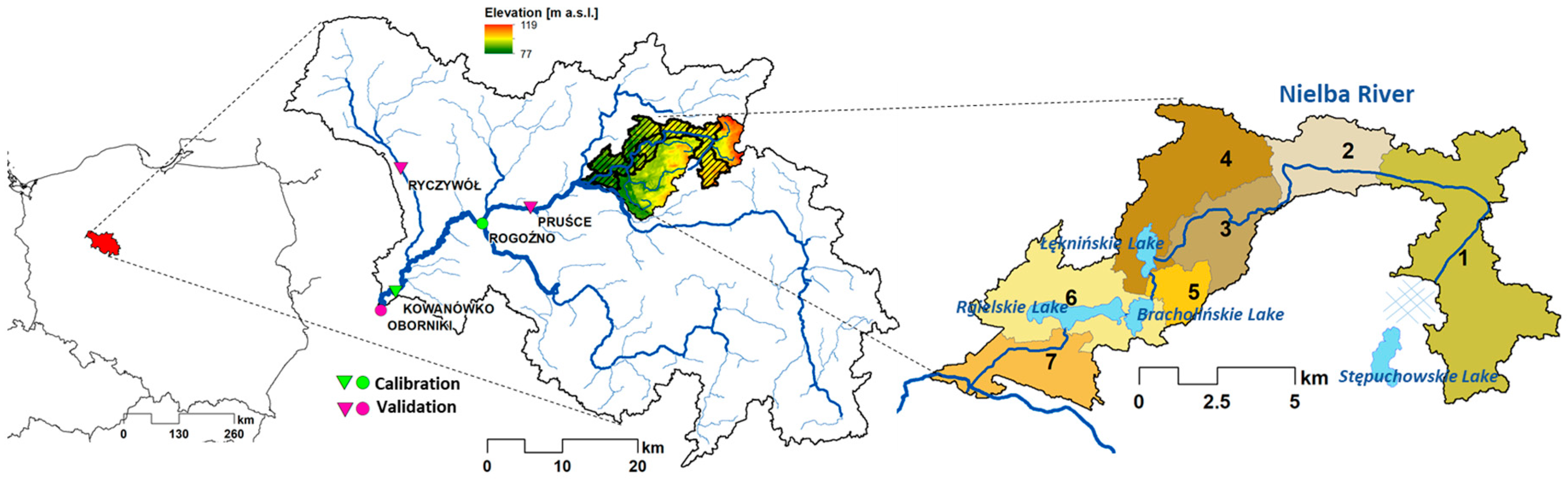
2.1. Study Area

The Nielba River catchment (158.6 km²) is located in central-western Poland and belongs to the Wełna River basin. Its gentle undulating topography is connected to moraine plains of the North Polish glaciation [39]. The Nielba River is characterized by a snow–rain hydrological regime with maximum flows in April caused by the spring snow melt. Following the spring high flow period, the water flow drops quickly to reach minimum values in September or at the turn of September and October. High flows caused by the summer and autumn rainfalls are rare in this catchment, since the average precipitation (500 mm) is one of the lowest in Poland. The winds from the western sector are predominant in this part of Poland, bringing in ocean air masses. The air average temperature is around 8.2 °C, and varies from 0 °C in winter to 19 °C during the summer. Snow cover lasts usually up to 50 days, while the number of frost days is in the range of 30 to 50. The vegetative season is one of the longest in Poland, starting at the end of March, and lasting about 220 days, which makes this area very suitable for agricultural activity. Indeed, this type of land use covers the majority of this catchment (82%), while forests cover 9%. Urbanized areas are scattered and occupy only 5%. The source of the Nielba River is localized in the vicinity of the Stępuchowskie Lake, which for many years has been a drainless area, while now it is connected to the river through a set of man-made canals. However, part of the Stępuchowskie Lake water outflows to the Wełna River catchment through a system of water gates. The Nielba River can be separated into two parts, the upper encompassing three riverine Sections (1–3, Figure 1), and the lower one from the Łęknińskie Lake, through the Bracholińskie and Regielskie Lakes, to the outlet of the Wełna River (Sections 4–7). However, the surface of these lakes has decreased in the last few decades to a different extent depending on the lake’s conditions. The least affected one is the Rgielskie Lake (0.4%), which is the largest lake in this catchment with an average depth of 5.3 m (max. 17 m), and due to its orientation is prone to wind mixing processes. The Bracholińskie Lake’s surface has decreased by 60% since the 1960s, and experienced serious ecological problems due to the impact of local manufacturing facilities [40]. Moreover, the Łęknińskie Lake’s conditions, with an average depth of 1.5 m (max. 2.8 m), and a low impact of wind mixing, favors an overgrowth process which affects the lake surface. As for the quality status, the Rgielskie Lake is classified as below good, the Bracholińskie Lake as eutrophic, while the Łęknińskie Lake as hypertrophic [41,42]. The quality of the Nielba River waters and its tributaries are heavily affected by agricultural runoff, a municipal wastewater point, and diffuse sources. Therefore, a high nutrient and organic matter concentration is observed in this river causing at least periodical degradation of the tributaries [42]. Moreover, the low flow rates (0.25 m³/s on average) of the streams do not guarantee a favorable degree of contaminant dilution, and cause low self-purification capacity of these waters [43]. In the upper part of the catchment, the water conditions are modified by the drainage systems, canals, and the presence of weirs and water gates.

2.2. Model Calibration and Validation

The Nielba River catchment model was extracted from the Wełna River SWAT model (ArcSWAT Version 2012.10_1.18), commissioned by the State Water Holding—Polish Waters (SWH-WP) under the project “Identification of pressures in water regions and river basin districts” [44]. Input data with their sources and resolution have been presented in Supporting Information S1. The SWAT model was calibrated, verified, and validated for quantitative (flow) and qualitative parameters (suspended sediment, total nitrogen, total phosphorus, and chlorophyll a) with a daily time step. For the quantitative calibration, daily flow data [45] were used for the period of 18 years (2001–2018) from three gauging stations: Two on the main course of the Wełna River (Pruśce and Kowanówko, Poland), and one on the Wełna River tributary Flinta (Ryczywół, Poland) (Figure 1). The qualitative model assessment was based on the State Monitoring System data from the Oborniki and Rogoźno stations on the Wełna River, and covered a period of 15 years (2001–2015). Calibration of the model was performed by the SWAT-CUP program [46] using the SUFI-2 algorithm (SWAT-CUP Version 5.2.1.1). The sensitivity analysis, performed with the Latin hypercube one-factor-at-a-time (LH-OAT) sampling approach, was used to identify the most influential estimation of constituent load (calibration) [29,47,48]. A formulated regression model was then used to estimate loads over a user-specified time interval (estimation). The sensitivity analysis was assessed using t-statistics by the Student’s t-test and p-value. Supporting Information S2 presented parameters that are sorted by p-value, in which a decreasing value indicates a more sensitive parameter. The t-statistics results, as the intensity and direction of parameters change during the analysis, are colored red for negative values (decrease), and blue for positive values (increase). The most sensitive parameters for flow were connected with surface runoff and infiltration intensity, time of water travel through to the lake or effectiveness of tillage systems. The nitrogen sensitivity analysis resulted in parameters, such as the rate of denitrification or nitrogen settling, benthic source of ammonium or soil characteristics. For phosphorus, the most sensitive parameters for this catchment were the ratio of enrichment with suspended sediment, phosphorus content in soils, and in groundwater or phosphorus availability index.

Calibration, verification, and validation results are presented as a table in Supporting Information S3. Three statistical parameters were used to assess model performance during the calibration process, coefficient of determination (R²), percent bias (PBIAS), and Kling–Gupta efficiency (KGE). For quantitative calibration, (Pruśce-Nielba and Ryczywół-tributary stations for 2004–2011), and verification (Pruśce and Ryczywół stations for 2012–2018) coefficients R² and KGE were in the range of 0.66–0.90 (Supporting Information S3), which classified the model performance generally as good and very good for the main course of the Wełna River, and satisfactory and good for its tributary (Flinta). A very good model performance was indicated by the PBIAS values (2–10%). During the validation procedure (Kowanówko station), all of the coefficient values rated the model’s performance for daily flow simulations as very good. Quantitative calibration and verification were performed for the Oborniki station for the periods of 2004–2011 and 2012–2015, respectively, while the validation procedure was executed for the Rogoźno station (2012 to 2015). Model performance achieved at the quantitative calibration process was assessed as good and very good. The obtained results for suspended sediment calibration and validation were very good and good, 0.52–0.81 and 20–22% for R²/KGE and PBIAS, respectively (Supporting Information S3-1). Statistic coefficients for total nitrogen ranged from 0.51 to 0.90 and from 12 to 20% for R²/KGE and PBIAS, respectively. Satisfactory performance was observed for total phosphorus. However, lower fit of simulation to observation for phosphorus is common as variability and temporal distribution patterns frequently affect the phosphorus peaks, rendering difficulties in simulations [49,50,51]. Due to the low data number of chlorophyll a observations for calibration and validation of this parameter, only the R² coefficient could be used. However, no value range has been offered in the published works to assess model performance for the chlorophyll a simulations.

2.3. Eutrophication Parameters Simulation

In the SWAT model, suspended algal biomass is assumed as directly proportional to chlorophyll a. Algal biomass transport and transformation in SWAT are divided into chlorophyll a loading from the land area, and chlorophyll a in-stream processes. Chlorophyll a loading to the stream is calculated based on a relationship between the nutrient enrichment index, chlorophyll a, and algal growth potential [2,52], according to Equation. (1) [52]:

$$\left(AGP+chla\right)\ast v_{surf}=f\ast {\left(\frac{TN}{TP}\right)}^g$$

(1)

where AGP is algal growth potential (µg chla/l); Chla is chlorophyll a concentration in surface runoff (µg chla/l); v_surf is the surface runoff flow rate (m³/s); TN/TP is the loading ratio; TN is the total nitrogen load (kg/d); TP is the total phosphorus load (kg/d); and f, g are the coefficient and exponent.

In the SWAT model, chlorophyll a concentration in surface runoff is calculated as a transformation of a simplified version of the Cluis [2] exponential function (Equations (2)–(4)) [52]:

$$chla=0 \mathrm{if} (v_{surf}<{10}^{-5 }{\mathsf{m}}^3/\mathsf{s}) or (TP and TN<{10}^{-6})$$

(2)

$$chla=\frac{0.5\ast {10}^{2.7}}{v_{surf}} \mathrm{if} (v_{surf}>{10}^{-5 }{\mathsf{m}}^3/\mathsf{s}) and (TP and TN>{10}^{-6})$$

(3)

$$chla=\frac{0.5\ast {10}^{0.5}}{v_{surf}} \mathrm{if} \left(v_{surf}>{10}^{-5} {\mathsf{m}}^3/\mathsf{s}, TP<{10}^{-6} and TN>{10}^{-6}\right)$$

(4)

The second stage in chlorophyll a modeling in SWAT involves in-stream processes. The growth, decay, and settling of algae form a part of a nutrient cycle. The simulation covers algal growth and settling. Chlorophyll a is assumed to be directly proportional to the algal biomass, according to Equation (5) [52]:

$$chla={\alpha }_0\ast algae$$

(5)

where chla is chlorophyll a concentration (µg chla/l); α₀ is algal biomass (µg chla/mg alg); and algae is algal biomass concentration (mg alg/l).

Growth and decay of algae (and proportionally chlorophyll a) are calculated as a function of environmental factors and nutrient supply. Parameters in base function are determined as the growth rate, the respiration rate, the settling rate, and the amount of algae present in the stream. The change in algal biomass for the daily time step is expressed by the following Equation Equation (6) [52]:

$$\mathsf{\Delta }algae=\left(\left({\mu }_a\ast algae\right)-\left({\rho }_a\ast algae\right)-\left(\frac{{\sigma }_l}{depth}\ast algae\right)\right)\ast TT$$

(6)

where Δalgae is the change in algal biomass concentration (mg alg/l); µ_a is the local specific growth rate of algae (day⁻¹); ρ_a is the local respiration or death rate of algae (day⁻¹); σ_l is the local settling rate for algae (m/day); depth is the depth of water in the channel (m); algae is the algal biomass concentration at the beginning of the day (mg alg/l); and TT is the flow travel time in the reach segment (day).

The local specific growth rate is calculated as a function of the nutrients availability, light, and temperature. The SWAT model first calculates the growth rate at 20 °C and then adjusts the growth rate for water temperature. There are three options of calculating the impact of nutrients and light on algal growth available in the SWAT model [47]. The multiplicative option was selected where the net effect on the local algal growth rate is determined by multiplication of the growth factors for light, nitrogen, and phosphorus together. The calculation is based on the biological basis of the multiplicative effects of enzymatic processes involved in photosynthesis (Equation (7)) [52]:

$${\mu }_{a20}={\mu }_{max}\ast FL\ast FN\ast FP$$

(7)

where µ_a20 is the local specific algal growth rate at 20 °C; µ_max is the maximum specific algal growth rate; FL is the algal growth attenuation factor for light; FN is the algal growth limitation factor for nitrogen; and FP is the algal growth limitation factor for phosphorus.

The algal growth limiting factor for light is calculated based on the mathematical relationship between the photosynthesis and light as the Monod half-saturation method [53] (Equation (8)) [52]:

$$F{L}_z=\frac{I_{phosyn,z}}{K_L+I_{phosyn,z}}$$

(8)

where FL_z is the algal growth attenuation factor for light at depth z; I_phosyn,z is the photosynthetically-active light intensity at depth z below the water surface (MJ/m²); and K_L is the half-saturation coefficient for light (MJ/m²).

Photosynthetically active light is radiation with a wavelength of 400–700 nm. The half-saturation coefficient for light is defined as the light intensity at which the algal growth rate is half of the maximum growth rate. The relationship between the light intensity and depth is defined by the Beer’s law and presented in (Equation (9)) [52]:

$$I_{phosyn,z}=I_{phosyn,hr}exp\left(-k_l\ast z\right)$$

(9)

where I_phosyn,hr is photosynthetically-active solar radiation reaching the ground/water surface during a specific hour on a given day (MJ/m²/hr); k_l is the light extinction coefficient (m⁻¹); and z is depth from the water surface (m).

The photosynthetically active solar radiation is calculated as (Equation (10)) [52]:

$$I_{phosyn,hr}=I_{hr}\ast f{r}_{phosyn}$$

(10)

where I_hr is the solar radiation reaching the ground/water surface during a specific hour on a given day (MJ/m²/hr); and fr_phosyn is the fraction of solar radiation that is photosynthetically active.

The photosynthetically active radiation, after Kiniry [54], usually falls in the range of 45 to 55% and is a function of cloud cover.

The algal growth limiting factor for nutrients is based on the Monod expression, as well. For nitrogen, the algal growth limitation factor uses both ammonia and nitrate, according to (Equation (11)) [52]:

$$FN=\frac{\left(C_{NO3}+C_{NH4}\right)}{\left(C_{NO3}+C_{NH4}\right)+K_N}$$

(11)

where FN is the algal growth limitation factor for nitrogen; C_NO3 is the concentration of nitrate in the reach (mg N/l); C_NH4 is the concentration of ammonium in the reach (mg N/l); and K_N is the Michaelis–Menten half-saturation constant for nitrogen (mg N/l).

For phosphorus, the use of the Monod expression is defined by (Equation (12)) [52]:

$$FP=\frac{C_{solP}}{C_{solP}+K_P}$$

(12)

where FP is the algal growth limitation factor for phosphorus; C_solP is the concentration of phosphorus in solution in the reach (mg P/l); and K_P is the Michaelis–Menten half-saturation constant for phosphorus (mg P/l).

The Michaelis–Menten half-saturation [55] constant defines the concentration of nitrogen or phosphorus at which algal growth is limited to 50% of the maximum growth. Usually, K_N ranges from 0.01 to 0.3 mg N/l, and K_P ranges from 0.001 to 0.05 mg P/l.

The algal growth rate is calculated with the use of the growth rate at 20 °C, based on the Streeter–Phelps formulation [56] (Equation (13)) [52]:

$${\mu }_a={\mu }_{a,20}\ast {1.047}^{\left(T_{water}-20\right)}$$

(13)

where µ_a is the local specific growth rate of algae (day⁻¹); µ_a,20 is the local specific growth rate of algae at 20 °C (day⁻¹); and T_water is the average water temperature for the day (°C).

The local respiration or death rate of algae represents the net effect of three processes: The endogenous respiration of algae, the conversion of algal phosphorus to organic phosphorus, and the conversion of algal nitrogen to organic nitrogen. The respiration rate is adjusted to the local water temperature using the relationship from Equation (14) [52]:

$${\rho }_a={\rho }_{a,20}\ast {1.047}^{\left(Twater-20\right)}$$

(14)

where ρ_a is the local respiration rate of algae; ρ_a,20 is the local algal respiration rate at 20 °C; and T_water is the average water temperature for the daily hours.

The net removal of algae due to settling is expressed as the local settling rate. The settling rate is adjusted to the local water temperature using (Equation (15)) [52]:

$${\sigma }_l={\sigma }_{l,20}\ast {1.047}^{\left(Twater-20\right)}$$

(15)

where σ_l is the local settling rate of algae; σ_l,20 is the local algal settling rate at 20 °C; and T_water is the average water temperature for the daily hours.

2.4. Data Selection and Treatment

The research aim achievement was performed by the mutual correlation analysis of parameters selected by their direct influence on chlorophyll a load simulations in the reach. The most important group factors stimulating algal growth and respiration, i.e., water temperature, solar radiation, and nutrient loads, were included. Moreover, water velocity was taken into consideration according to its impact on water travel time in a section, as well as chlorophyll a land delivery from a particular sub-basin area, as parameters influencing river eutrophication.

Following these assumptions seven parameters were selected:

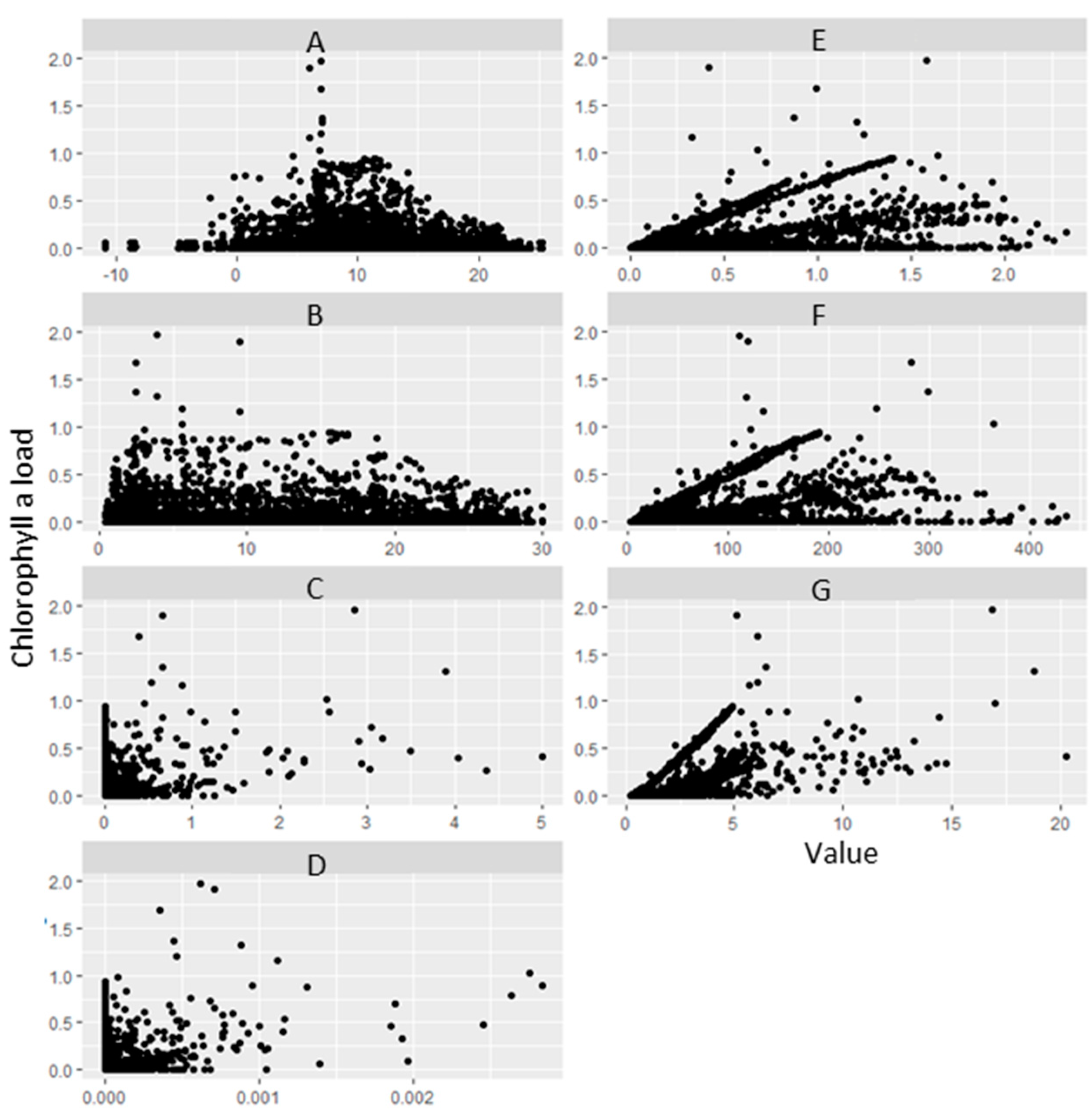
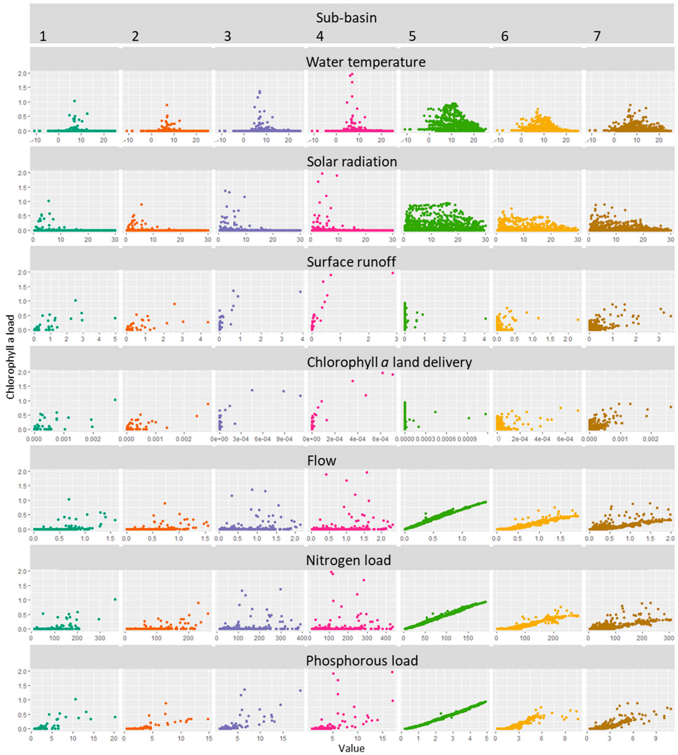
• Water temperature (°C);
• Solar radiation (MJ/m²);
• Surface runoff (mm);
• Chlorophyll a land delivery (µg chla/l);
• Flow (m³/s);
• Total nitrogen transported with the water into the reach (kg N/day);
• Total phosphorus transported with the water into the reach (kg P/day).

The analysis for the Nielba River was performed for simulations years 2005–2007. The final choice of the time period was dictated by the meteorological and hydrological differentiation of the selected years. This period covers a hydrologically wet (2007), medium (2005), and relatively dry year (2006) [45]. As for the winter thermal conditions, which is important due to the vegetative season length, the winter of 2005 was considered slightly warm, for 2006 very cool, and for 2007 extremely warm when compared with the multi-year average temperature in this area [45]. Therefore, the selected 3-year period was considered representative and subjected to further analyses.

The results of the SWAT simulations with a daily step for the seven sections of the Nielba River (Figure 1) were retrieved from the model output and examined. The chlorophyll a load results were analyzed in relation to the selected parameters, as displayed in Figure 2. The analyses were performed in a two-stage approach: (i) General correlation analysis for the entire Nielba River dataset to assess river trends, and (ii) river sections correlation analysis for each sub-basin separately to assess the impact of local conditions along the watercourse.

3. Results

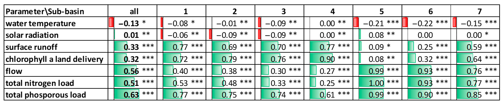
3.1. General Correlation Analysis

In the analyzed period (2005–2007), daily chlorophyll a loads ranged from 0 to 2 kg/d. However, the 95th percentile value was equal to 0.47 kg/d, and most of the results were below 0.032 kg/d. Only eight values were considered outliers and exceeded 1 kg/d. The relationship between chlorophyll a loads and water temperature has been presented in Figure 2A. The SWAT model calculated temperature values that ranged from −11 to 25 °C. However, temperatures below 0 °C were excluded from further analyses as not favorable for eutrophication processes. Chlorophyll a loads above the 95th percentile value coincided with water temperatures between 5 and 15 °C, while the outliers occurred at 5 °C. The solar radiation ranged from 0 to 30 MJ/m², and no significant relationship was observed, apart from a lower frequency of the chlorophyll a loads above the 95th percentile for solar radiation higher than 20 MJ/m² (Figure 2B). The chlorophyll a outliers were simulated for the radiation of 3–10 MJ/m². The simulated surface runoff values were in the range of 0 to 5 mm/d, while chlorophyll a land delivery from particular sub-catchments ranged from 0 to 0.003 µg chla/l. For both parameters, no visible relationship with chlorophyll a loads has been observed (Figure 2C,D), and loads above the 95th percentile appeared through the whole range of values. For the next three parameters, i.e., flow (0–24 m³/s), total nitrogen (3–430 kg/d), and total phosphorus loads (0.2–21 kg/d), the distribution showed a similar result pattern (Figure 2E,G). Groups of points with a higher correlation to chlorophyll a, and groups of points with a higher dispersion, could be distinguished. Moreover, the elevated chlorophyll a loads appeared through the whole range of the discussed parameters.

The mutual interdependence of all the studied parameters was analyzed through the correlation matrix (Figure 3) for daily values in the period of 2005–2007, and all seven sections of the Nielba River. The chlorophyll a loads (7665 results) were related one-by-one with the other seven parameters, and the significance of these relationships was assessed through the correlation coefficient (R) and probability values (p-value). The highest R values were observed between flow and nutrient loads, reaching 0.96 and 0.73 for the total nitrogen and phosphorus, respectively. The correlation of the flow and nutrients is influenced by the extent to which nutrients depend on the quality of water carried from the previous profile, and the extent on impact of the processes in a given sub-catchment area. As for the outliers, a small number was observed for the relationship between flow and total nitrogen, and a greater number of outliers for total phosphorus, especially in the high load ranges. Furthermore, due to the internal correlation, a high R value (0.74) has been observed between surface runoff and chlorophyll a land delivery, although a clear separation of points into two groups could be observed. One with a positive quasi-linear correlation between both parameters, and the second with high values of chlorophyll a land delivery (>0.0014 µg chla/l), and surface runoffs in the range of 0.08–0.30 mm (90–95th percentile). Both groups were subjected to further analyses. No apparent correlation has been observed between solar radiation and the analyzed parameters, in addition to water temperature where the correlation coefficient is 0.67. The figure interpretation shows that up to a water temperature of 0 °C, solar radiation is at a similar level. Above this temperature, solar radiation and temperature are directly proportional.

The direct correlation between chlorophyll a load, and total phosphorus and nitrogen were equal to 0.63 and 0.51, respectively. Again, the separation of points into two groups could be observed. One with a quasi-linear increase of chlorophyll a loads with total nutrient loads increase, and the second with stable chlorophyll a loads despite of the nutrient loads increase. Both groups were subjected to further analyses. Lower, although still statistically significant correlation, was observed for chlorophyll a loads and surface runoff (R = 0.33), as well as chlorophyll a land delivery (R = 0.32). No significant correlation has been observed between chlorophyll a load, and water temperature and solar radiation.

3.2. River Sections Correlation Analysis

The second stage of the research is the dataset analysis for identification of obtained dependencies. The basic division of the point cloud is the separation by the Nielba River sections. The chlorophyll a loads in the relationship with the analyzed parameters were shown in Figure 2. The results, presented as a joined dataset (Figure 2 and Figure 3), were detailed through an analysis on the sub-basin level. The chlorophyll a load relation to other parameters for data separated by sub-basins are presented by separate charts (Figure 4). The groups of points with a linear relationship between chlorophyll a load, observed for flow or nutrient loads in joined data analysis, correspond with the individual sub-basins, as well as the data with a large dispersion. The comparison of Figure 2 and Figure 4 suggests that in terms of the obtained simulation results, the Nielba River is divided into two parts. For sub-basins 1–4, the simulation results for chlorophyll a loads are dependent on different conditions and show distinct trends for sub-basins 5–7 (sub-basin division in Figure 1).

A detailed analysis of the correlation of chlorophyll a load and the studied parameters for individual sub-basins is presented in

Table 1. The R values for the relations of chlorophyll a and selected parameters (p-value below 0.001—“***”, between 0.001 and 0.01—“**”, 0.01–0.05—“*”,and higher than 0.1 without a symbol).

, while the relationships for all parameters are included as correlation matrices in Supporting Information S4.

Sections 1–4 cover the river sources area through the upper Nielba sections to the first flow-through lake. Correlation coefficients for the analyzed parameters differ from the combined dataset results. Similar trends are observed in the mentioned sections. The correlation of chlorophyll a load to flow is lower than all the sub-basins dataset, and is decreasing along with the subsequent sections (R for Section 1 is equal to 0.40, and 0.27 for Section 4). The chlorophyll a load correlation to total phosphorus load increased to 0.77 for Section 1, and is decreasing through all sections to 0.61 for Section 4. The correlation of phosphorus load and surface runoff significantly increased in Section 1 (R = 0.96), and is decreasing to 0.46 in Section 4. The correlation of total nitrogen load and surface runoff is equal to R = 0.45 for Section 1, and is suddenly decreasing for the further sections to a nonsignificant value in Section 4, where the correlation coefficient of nitrogen load and flow is the highest along the upper Nielba and close to 1. The chlorophyll a load in this area is also strongly correlated with surface runoff and chlorophyll a land delivery, the R coefficients are from 0.69 to 0.77 and from 0.72 to 0.90, respectively. In sub-basins 3 and 4, the surface runoff values decreased, except for the individual peaks seen in Supporting Information S4-3, column 4. For chlorophyll a loads, high peaks are also observed for sub-basins preceding the lake (Supporting Information S4-4, column 1).

The statistics from sub-basin 5 indicate a radical change compared with the results for the upper Nielba. Both chlorophyll a and nutrient loads are strongly related to flow. Pollutants in this section come from the Łęknińskie Lake. A significant nutrient load decrease is noted and the episodic peaks of loads of chlorophyll a, characteristic from the previous sub-basins are reduced—the point cloud is more uniform (Supporting Information S4-5, column 1). The surface runoff, expressed as the analyzed unit, is generally small, except for individual peaks (Supporting Information S4-5, column 4). In sub-basin 6, the correlation of chlorophyll a and nutrient loads to flow is high, as well. On the contrary, for sub-basin 5, a relationship of those parameters to the surface runoff appeared, and for the total phosphorus R is equal to 0.43. This value is similar to the result for this correlation in the joined dataset. Plots for the surface runoff (Supporting Information S4-6, column 4) show the least influence of outliers, and a more linear relationship of surface runoff to flow and nutrients. Sub-basin 7 is a Nielba estuary into the Wełna River. The high correlation of chlorophyll a load to flow (R = 0.76), and nutrient loads (0.77 for nitrogen and 0.85 for phosphorus) persist. In both Sections 6 and 7, a very high correlation of flow and nutrient loads were noted (up to R = 0.99). Significantly higher is the correlation of chlorophyll a loads and surface runoff, and chlorophyll a land delivery, with R equal to 0.64 and 0.59, respectively, at the expense of a decrease in the correlation with flow.

4. Discussion

The Nielba River localization and its conditions make its water prone to eutrophication processes. The majority of agricultural land use and the high initial values of nutrients in soils are responsible for possible water fertility. Additionally, the climate conditions contribute to the long vegetative season, which favors the intensification of primary production [57,58]. The Nielba River catchment stream density is relatively high, which is influenced by a large number of small watercourses, most of which are periodic. The water travel time and outflow disturbances in the tributaries may lead to forming zones of algal growth intensification, and can be an additional source into the main stream. Additionally, the orientation of the lakes’ axis opposite to the prevailing wind direction causes low susceptibility to wind mixing of the waters [59,60]. Therefore, the Nielba River is a good example for the analysis of eutrophication processes. Since there is no monitoring data available for this watercourse, modeling remains a primary tool to evaluate chlorophyll a load changes and dependencies.

The first stage of analysis, when simulation results were analyzed as a combined cloud of points from all sections, resulted in trends observed generally for the whole Nielba River. First, there was no correlation observed for chlorophyll a loads to temperature or solar radiation, despite the theoretical impact of these parameters on algal growth. However, these parameters appear in formulas in SWAT modeling indirectly (Equations (1)–(15)). Solar radiation is a parameter that is included in the algal growth limiting factor for light. Water temperature is included in the algal respiration and algal settling rates. The way temperature and solar radiation are implemented in the equations do not show a significant impact when the dataset is studied generally, thus detailed data separation are needed.

A positive correlation occurred for the chlorophyll a load relationship to surface runoff (R = 0.33), and consequently chlorophyll a land delivery (R = 0.32). The correlation coefficient for these parameters indicates that a part of chlorophyll a in the river is associated with chlorophyll a delivery from the land. According to the method of chlorophyll a land delivery simulation in SWAT (Equations (1)–(4)), this parameter is calculated depending on the value of the surface runoff. This correlation confirms the dependence of chlorophyll a loads in small rivers on surface erosion. However, for the joined dataset, the obtained results of the R value are low. While the correlation of chlorophyll a load and flow, which may indicate that the appearance of chlorophyll a in the river section is caused by carrying it from the sections above by flowing water, exceeded R = 0.5. For the joined dataset, this impact occurred more strongly. As for the relationship between chlorophyll a and nutrient loads, the correlation with phosphorus is higher than with nitrogen (R for phosphorus is 0.63, and for nitrogen is 0.51). Additionally, the simulation results for phosphorus loads correlate with surface runoff at R = 0.49. The source of nutrients in river water is mainly erosion, soil leaching, and point discharges. The phosphorus is more likely connected with suspended sediment and its transport is dependent on surface erosion when nitrogen is usually transported in soluble forms by leaching. Furthermore, in the studied catchment, the sewage network is very limited [34]. This problem was incorporated into the model and leaky septic tanks were introduced. In SWAT, the chlorophyll a load simulation method equations for both nutrients were included as limiting factors (Equations (11) and (12)). The highest correlation of chlorophyll a loads with phosphorus loads, than with nitrogen loads may indicate that the phosphorus has the stronger limiting function in this case.

The second stage of the research relies on separate analyses for each part of the studied system. The obtained results indicated different trends in chlorophyll a simulation for the particular Nielba River sections. In the upper sections, the chlorophyll a loads depended on the surface runoff and nutrients leaching from the soil into the river water, especially for phosphorus where R for chlorophyll a and phosphorus loads was up to 0.77. The high correlation of total phosphorus load with surface runoff suggests a high degree of phosphorus leaching from the soil in this part of the catchment area. The phosphorus is leached from soils to a greater extent as a result of surface erosion and sorption on soil particles than through groundwater, as in the case of nitrogen [61]. The correlation of flow and surface runoff among the studied sections is highest in the upper Nielba (R = 0.31), which suggests a relationship to flow and precipitation, however, not strong. The SWAT modeling for the river source sections, to some extent, makes hydrological and chemical conditions strictly dependent on torrential rains. In relation to values in the source sections, chlorophyll a loads increased along the river course. The simulation of chlorophyll a load increase depends on a potential algal growth, for which equations take into account environmental factors. The chlorophyll a land delivery equations include only the surface runoff value. This time the peak depends on the dominant algal species in the water. In the studied river, algae dominated with a very wide temperature tolerance and the highest abundance in cool water [62].

Another important tendency observed in the results is the influence of the Łęknińskie Lake. The sections below this lake are characterized by different trends than the upper Nielba sections [38]. The flow and nutrient loads decrease, and the chlorophyll a load increases. In the lake, the primary production causes nutrient depletion and chlorophyll a increases in the water outflowing the lake, and the inflowing Section 5 of the Nielba River. The nutrient loads are closely related to the flow, which in this case is the lake outflow. The time of water retention in the lake allowed algae to develop. The algal growth caused the biological purification of water from the nutrients. The Łęknińskie Lake is very shallow and extensive in the sub-basin area with a hypertrophic status. The sub-basin 5 has a small area and is a short river fragment connecting the lakes. The model reflects the natural situation. However, in an exaggerated way, which is reflected in the very high values of the correlation coefficient. For the next sub-basin charts (River Section 6), the visual assessment suggests a more probable representation of the actual values in the environment. The section is longer and contains two lakes with a better trophic status. The Rgielskie Lake is five times deeper than Łęknińskie. The chlorophyll a load decreases and its relationship to surface runoff increases. The two lakes downstream from Łęknińskie do not cause the escalation of the algal content in the water flowing to its final section. The interpretation of the results suggests that the influence of Łęknińskie Lake, which radically changed the relationship of the examined parameters, weakens with each river section and the correlations start to return to the values from the upper Nielba, where the chlorophyll a loads are strongly influenced by surface runoff. At the estuary, the major impact on chlorophyll a loads has water inflowing from the previous section. However, the impact of nutrient soil leaching is still significant (correlation coefficient for chlorophyll a load and surface runoff is 0.59). The modeling of the impact of the Łeknińskie Lake on water quality of the Nielba River, according to the actual situation, may be exaggerated. However, the main conditions and processes in this river are reflected at a satisfying level. Model verification of chlorophyll a load trends in this area needs a detailed field study. However, for comparative space-time analyses or scenario studies, the obtained results are considered sufficient.

The implemented approach has certain limitations. The simulation of chlorophyll a in the SWAT model can be only performed for the unmonitored sub-basin constituting part of the catchment for which the calibration procedure was successfully implemented. Consequently, in addition to an extensive input dataset, the field sourced observation and data on the eutrophication phenomenon for a particular system should be available to evaluate the SWAT model performance. Unfortunately, the quantity and quality of these data are usually quite limited, due to the poor localization or time frequency of monitoring efforts. Additionally, chlorophyll a measurements are conducted mainly in the spring–summer season, while algal species developing in cold temperatures are usually neglected in the monitoring networks. Therefore, the temporal analyses of the chlorophyll a peak occurrence should be carefully verified with field information. Moreover, the SWAT model simulates algae as one homogeneous group, without differentiation of species, optimal growth or transport condition⁴⁷. However, the peaks of algal density (and directly proportional chlorophyll a loads) may occur in different seasons. The verification of the modeled time of maximum primary production with the local climatic and hydrological conditions, and probable species composition, allow for a preliminary assessment of the reliability of the obtained results.

In the chlorophyll a load simulations, apart from the peak occurrence, their size should also be subjected to analyses, especially in the context of outliers’ presence. Particularly, since the SWAT model evaluation is performed by statistic measure values which are strongly influenced by outliers. The SWAT model, especially for certain parameters, such as phosphorus or chlorophyll a, often overestimates their loads that outlie significantly from the dataset. Therefore, in situations where the exact quantity analysis is the aim of the study, the weight of outliers must be reduced⁴⁵. In other cases, the outlier presence can signify local conditions, e.g., effects of the rain–snow regime in the studied river. Additionally, it should also be mentioned that the applied correlation analyses have also some limitations when the simulated eutrophication parameters are taken into consideration. As observed for the Nielba River system, the correlation coefficients were close to 1 in some cases. Since this perfect relationship between chlorophyll a and the studied parameters does not occur in the real environment, it should be noted that the SWAT model produces only an approximation of real conditions. However, when calibration, verification, and validation processes are assumed to be at a satisfactory level, modeling efforts could be assessed as a sufficient real processes’ reflection. Therefore, the obtained results should be analyzed with a certain limit of uncertainty.

5. Conclusions

The obtained results show that the SWAT model can be successfully used for chlorophyll a simulations. Moreover, tracking relationships between chlorophyll a loads and the selected parameters can be very helpful in exploration of the dominant trends of chlorophyll a simulations in riverine conditions and can be an effective tool for chlorophyll a simulation study for an unmonitored watercourse. The analyses on the combined dataset for the Nielba River, showed a strong correlation of chlorophyll a to flow and surface runoff, but had no relationship with temperature or solar radiation. This may indicate that the regularities of lentic systems do not directly translate into lotic patterns. However, it is also possible, that the impact of temperature or solar radiation, in the ranges presented in this study, are additionally belittled by the construction of a mathematical formula used in the model. In any way, this phenomenon should be taken into consideration in systems where ranges of these parameters are significantly broader.

The separation of the dataset into the river section pattern, helped in the identification of the impact of local conditions on chlorophyll a load variability. For the studied river, changes induced by the presence of lakes shall be considered as the most important factor affecting the chlorophyll a simulations. Inflow lakes, as well as dammed reservoirs, change water travel time in a pertinent system section. Therefore, nutrient loads, as well as primary production dynamics, are subjected to alterations. Since the SWAT model responds accurately to features of a particular water body and well reflects the impact of the most important parameters, the obtained information can be implemented in other models focusing on eutrophication simulations for the detailed biological analysis.

References

1. Boynton, W.R.; Kemp, W.M.; Keefe, C.W.A. Comparative Analysis of Nutrients and Other Factors Influencing Estuarine Phytoplankton Production. In Estuarine Comparisons; Kennedy, V.S., Ed.; Academic Press: Cambridge, MA, USA, 1982; pp. 69–90. [Google Scholar] [CrossRef]
2. Cluis, D.; Couture, P.; Bégin, R.; Visser, S.A. Potential Eutrophication Assessment in Rivers; Relationship between Produced and Exported Loads. Swiss J. Hydrol. 1988, 50, 166–181. [Google Scholar] [CrossRef]
3. Minaudo, C.; Meybeck, M.; Moatar, F.; Gassama, N.; Curie, F. Eutrophication Mitigation in Rivers: 30 Years of Trends in Spatial and Seasonal Patterns of Biogeochemistry of the Loire River (1980–2012). Biogeosciences 2015, 12, 2549–2563. [Google Scholar] [CrossRef] [Green Version]
4. Dodds, W.K.; Smith, V.H. Nitrogen, Phosphorus, and Eutrophication in Streams. Inland Waters 2016, 6, 155–164. [Google Scholar] [CrossRef]
5. Ménesguen, A.; Desmit, X.; Dulière, V.; Lacroix, G.; Thouvenin, B.; Thieu, V.; Dussauze, M. How to Avoid Eutrophication in Coastal Seas? A New Approach to Derive River-Specific Combined Nitrate and Phosphate Maximum Concentrations. Sci. Total Environ. 2018, 628–629, 400–414. [Google Scholar] [CrossRef] [Green Version]
6. Le Moal, M.; Gascuel-Odoux, C.; Ménesguen, A.; Souchon, Y.; Étrillard, C.; Levain, A.; Moatar, F.; Pannard, A.; Souchu, P.; Lefebvre, A.; et al. Eutrophication: A New Wine in an Old Bottle? Sci. Total Environ. 2019, 651, 1–11. [Google Scholar] [CrossRef] [Green Version]
7. Tang, X.; Li, R.; Han, D.; Scholz, M. Response of Eutrophication Development to Variations in Nutrients and Hydrological Regime: A Case Study in the Changjiang River (Yangtze) Basin. Water 2020, 12, 1634. [Google Scholar] [CrossRef]
8. Kováčová, V. Assessment of Surface Water Eutrophication at Žitný Ostrov Region. Acta Hydrol. Slovaca 2020, 21, 65–73. [Google Scholar] [CrossRef]
9. Boeykens, S.P.; Piol, M.N.; Samudio Legal, L.; Saralegui, A.B.; Vázquez, C. Eutrophication Decrease: Phosphate Adsorption Processes in Presence of Nitrates. J. Environ. Manag. 2017, 203, 888–895. [Google Scholar] [CrossRef]
10. Dalu, T.; Wasserman, R.J.; Magoro, M.L.; Froneman, P.W.; Weyl, O.L.F. River Nutrient Water and Sediment Measurements Inform on Nutrient Retention, with Implications for Eutrophication. Sci. Total Environ. 2019, 684, 296–302. [Google Scholar] [CrossRef]
11. Reynolds, C.S. The Ecology of Phytoplankton; Cambridge University Press: Cambridge, UK, 2006. [Google Scholar]
12. Paerl, H.W.; Valdes, L.M.; Peierls, B.L.; Adolf, J.E.; Harding, L.W., Jr. Anthropogenic and Climatic Influences on the Eutrophication of Large Estuarine Ecosystems. Limnol. Oceanogr. 2006, 51, 448–462. [Google Scholar] [CrossRef] [Green Version]
13. Degobbis, D.; Precali, R.; Ivancic, I.; Smodlaka, N.; Fuks, D.; Kveder, S. Long-Term Changes in the Northern Adriatic Ecosystem Related to Anthropogenic Eutrophication. Int. J. Environ. Pollut. 2000, 13, 495–533. [Google Scholar] [CrossRef]
14. Nazari-Sharabian, M.; Ahmad, S.; Karakouzian, M. Climate Change and Eutrophication: A Short Review. Eng. Technol. Appl. Sci. Res. 2018, 8, 3668–3672. [Google Scholar] [CrossRef]
15. Charlton, M.B.; Bowes, M.J.; Hutchins, M.G.; Orr, H.G.; Soley, R.; Davison, P. Mapping Eutrophication Risk from Climate Change: Future Phosphorus Concentrations in English Rivers. Sci. Total Environ. 2018, 613–614, 1510–1526. [Google Scholar] [CrossRef] [PubMed] [Green Version]
16. Krasa, J.; Dostal, T.; Jachymova, B.; Bauer, M.; Devaty, J. Soil Erosion as a Source of Sediment and Phosphorus in Rivers and Reservoirs—Watershed Analyses Using WaTEM/SEDEM. Environ. Res. 2019, 171, 470–483. [Google Scholar] [CrossRef]
17. Strokal, M.; Kahil, T.; Wada, Y.; Albiac, J.; Bai, Z.; Ermolieva, T.; Langan, S.; Ma, L.; Oenema, O.; Wagner, F.; et al. Cost-Effective Management of Coastal Eutrophication: A Case Study for the Yangtze River Basin. Resour. Conserv. Recycl. 2020, 154, 104635. [Google Scholar] [CrossRef]
18. Boyer, J.N.; Kelble, C.R.; Ortner, P.B.; Rudnick, D.T. Phytoplankton Bloom Status: Chlorophyll a Biomass as an Indicator of Water Quality Condition in the Southern Estuaries of Florida, USA. Ecol. Indic. 2009, 9 (Suppl. S6), S56–S67. [Google Scholar] [CrossRef]
19. Hu, W.; Li, C.; Ye, C.; Wang, J.; Wei, W.; Deng, Y. Research Progress on Ecological Models in the Field of Water Eutrophication: CiteSpace Analysis Based on Data from the ISI Web of Science Database. Ecol. Model. 2019, 410, 108779. [Google Scholar] [CrossRef]
20. Burigato Costa, C.M.d.s.; da Silva Marques, L.; Almeida, A.K.; Leite, I.R.; de Almeida, I.K. Applicability of Water Quality Models around the World—A Review. Environ. Sci. Pollut. Res. 2019, 26, 36141–36162. [Google Scholar] [CrossRef]
21. Costa, C.M.d.S.B.; Leite, I.R.; Almeida, A.K.; de Almeida, I.K. Choosing an Appropriate Water Quality Model—a Review. Environ. Monit. Assess. 2021, 193, 38. [Google Scholar] [CrossRef]
22. Park, Y.; Cho, K.H.; Park, J.; Cha, S.M.; Kim, J.H. Development of Early-Warning Protocol for Predicting Chlorophyll-a Concentration Using Machine Learning Models in Freshwater and Estuarine Reservoirs, Korea. Sci. Total Environ. 2015, 502, 31–41. [Google Scholar] [CrossRef]
23. Cole, T.M.; Wells, S.A. CE-QUAL-W2: A Two-Dimensional, Laterally Averaged, Hy-Drodynamic and Water Quality Model, Version 3.1; Instruction Report EL-03-1; US Army Engi-neering and Research Development Center: Vicksburg, MS, USA, 2003. [Google Scholar]
24. Walstra, D.J.R. Description of TRANSPOR2004 and Implementation in Delft3D-ONLINE: Interim Report; Rijkswaterstaat Institute for Coast and Sea: Rotterdam, The Netherlands, 2004. [Google Scholar]
25. Park, R.A.; Clough, J.S.; Wellman, M.C. AQUATOX: Modeling Environmental Fate and Ecological Effects in Aquatic Ecosystems. Ecol. Model. 2008, 213, 1–15. [Google Scholar] [CrossRef]
26. Parveen, N.; Singh, S. Application of Qual2e Model for River Water Quality Modelling. Int. J. Adv. Res. Innov. 2016, 4, 429–432. [Google Scholar]
27. Schwarz, G.; Hoos, A.B.; Alexander, R.B.; Smith, R.A. Section 3. The SPARROW Surface Water-Quality Model—Theory, Application and User Documentation; Techniques and Methods; USGS Numbered Series 6-B3; U.S. Geological Survey: Reston, VA, USA, 2006; Volume 6-B3. [CrossRef] [Green Version]
28. Srinivas, R.; Singh, A.P. An Integrated Fuzzy-Based Advanced Eutrophication Simulation Model to Develop the Best Management Scenarios for a River Basin. Environ. Sci. Pollut. Res. 2018, 25, 9012–9039. [Google Scholar] [CrossRef] [PubMed]
29. Duda, P.; Hummel, P.; Donigian, J.A.; Imhoff, J. BASINS/HSPF: Model Use, Calibration, and Validation. Trans. ASABE 2012, 55, 1523–1547. [Google Scholar] [CrossRef]
30. Arnold, J.; Moriasi, D.; Gassman, P.; Abbaspour, K.; White, M.; Srinivasan, R.; Santhi, C.; Harmel, R.; van Griensven, A.; Van Liew, M.; et al. SWAT: Model Use, Calibration, and Validation. Trans. ASABE 2012, 55, 1491–1508. [Google Scholar] [CrossRef]
31. Morelli, B.; Hawkins, T.R.; Niblick, B.; Henderson, A.D.; Golden, H.E.; Compton, J.E.; Cooter, E.J.; Bare, J.C. Critical Review of Eutrophication Models for Life Cycle Assessment. Environ. Sci. Technol. 2018, 52, 9562–9578. [Google Scholar] [CrossRef]
32. Debele, B.; Srinivasan, R.; Parlange, J.-Y. Coupling Upland Watershed and Downstream Waterbody Hydrodynamic and Water Quality Models (SWAT and CE-QUAL-W2) for Better Water Resources Management in Complex River Basins. Environ. Model. Assess. 2008, 13, 135–153. [Google Scholar] [CrossRef]
33. Grizzetti, B.; Bouraoui, F.; Granlund, K.; Rekolainen, S.; Bidoglio, G. Modelling Diffuse Emission and Retention of Nutrients in the Vantaanjoki Watershed (Finland) Using the SWAT Model. Ecol. Model. 2003, 169, 25–38. [Google Scholar] [CrossRef]
34. Santhi, C.; Arnold, J.G.; Williams, J.R.; Dugas, W.A.; Srinivasan, R.; Hauck, L.M. Validation of the Swat Model on a Large Rwer Basin with Point and Nonpoint Sources1. JAWRA J. Am. Water Resour. Assoc. 2001, 37, 1169–1188. [Google Scholar] [CrossRef]
35. Krysanova, V.; Arnold, J.G. Advances in Ecohydrological Modelling with SWAT—A Review. Hydrol. Sci. J. 2008, 53, 939–947. [Google Scholar] [CrossRef]
36. Imani, S.; Delavar, M.; Niksokhan, M.H. Identification of Nutrients Critical Source Areas with SWAT Model under Limited Data Condition. Water Resour. 2019, 46, 128–137. [Google Scholar] [CrossRef]
37. Lee, J.; Woo, S.-Y.; Kim, Y.-W.; Kim, S.-J.; Pyo, J.; Cho, K.H. Dynamic Calibration of Phytoplankton Blooms Using the Modified SWAT Model. J. Clean. Prod. 2022, 343, 131005. [Google Scholar] [CrossRef]
38. Orlińska-Woźniak, P.; Szalińska, E.; Jakusik, E.; Bojanowski, D.; Wilk, P. Biomass Production Potential in a River under Climate Change Scenarios. Environ. Sci. Technol. 2021, 55, 11113–11124. [Google Scholar] [CrossRef]
39. Gąbka, M.; Jakubas, E.; Joniak, T.; Golski, J. Rzeki Wełna i Flinta—Charakterystyka Obiektów Badań, Ich Położenie i Granice Zlewni; Bogucki Wydawnictwo Naukowe: Poznań, Poland, 2014; pp. 21–33. [Google Scholar]
40. Budzynska, A.; Dondajewska-Pielka, R.; Rosinska, J.; Kowalczewska-Madura, K.; Kozak, A.; Bogucki Wydawnictwo Naukowe. Ekosystemy Wodne: Funkcjonowanie, Znaczenie, Ochrona i Rekultywacja: Monografia Wydana z Okazji Jubileuszu 70. Urodzin prof. dr. hab. Ryszarda Goldyna; Bogucki Wydawnictwo Naukowe: Poznan, Poland, 2019. [Google Scholar]
41. Dondajewska, R.; Gołdyn, R.; Kowalczewska-Madura, K.; Kozak, A.; Romanowicz-Brzozowska, W.; Rosińska, J.; Budzyńska, A.; Podsiadłowski, S. Hypertrophic Lakes and the Results of Their Restoration in Western Poland. In Polish River Basins and Lakes—Part II: Biological Status and Water Management; Korzeniewska, E., Harnisz, M., Eds.; Springer International Publishing: Cham, Switzerland, 2020; pp. 373–399. [Google Scholar] [CrossRef]
42. GIOŚ. Monitoring Wód. Available online: https://www.gios.gov.pl/pl/stan-srodowiska/monitoring-wod (accessed on 5 April 2022).
43. Messyasz, B.; Szczuka, E.; Kaznowski, A.; Burchardt, L. Phytoseston and Heterotrophic Bacteria in the Assessment of the Waters in the Wełna and Nielba Rivers. Oceanol. Hydrobiol. Stud. 2010, 39, 45–63. [Google Scholar] [CrossRef]
44. O Wodach Polskich. Available online: https://www.wody.gov.pl/ (accessed on 5 April 2022).
45. Strona główna|Instytut Meteorologii i Gospodarki Wodnej—Państwowy Instytut Badawczy. Available online: https://www.imgw.pl/ (accessed on 5 April 2022).
46. Abbaspour, K.C.; Rouholahnejad, E.; Vaghefi, S.; Srinivasan, R.; Yang, H.; Kløve, B. A Continental-Scale Hydrology and Water Quality Model for Europe: Calibration and Uncertainty of a High-Resolution Large-Scale SWAT Model. J. Hydrol. 2015, 524, 733–752. [Google Scholar] [CrossRef] [Green Version]
47. Park, G.A.; Park, J.Y.; Joh, H.K.; Lee, J.W.; Ahn, S.R.; Kim, S.J. Evaluation of Mixed Forest Evapotranspiration and Soil Moisture Using Measured and Swat Simulated Results in a Hillslope Watershed. KSCE J. Civ. Eng. 2014, 18, 315–322. [Google Scholar] [CrossRef]
48. Khoi, D.N.; Thom, V.T. Parameter Uncertainty Analysis for Simulating Streamflow in a River Catchment of Vietnam. Glob. Ecol. Conserv. 2015, 4, 538–548. [Google Scholar] [CrossRef] [Green Version]
49. Lu, S.; Kronvang, B.; Audet, J.; Trolle, D.; Andersen, H.E.; Thodsen, H.; van Griensven, A. Modelling Sediment and Total Phosphorus Export from a Lowland Catchment: Comparing Sediment Routing Methods. Hydrol. Process. 2015, 29, 280–294. [Google Scholar] [CrossRef]
50. Ostojski, M.S.; Gębala, J.; Orlińska-Woźniak, P.; Wilk, P. Implementation of Robust Statistics in the Calibration, Verification and Validation Step of Model Evaluation to Better Reflect Processes Concerning Total Phosphorus Load Occurring in the Catchment. Ecol. Model. 2016, 332, 83–93. [Google Scholar] [CrossRef]
51. Bauwe, A.; Eckhardt, K.-U.; Lennartz, B. Predicting Dissolved Reactive Phosphorus in Tile-Drained Catchments Using a Modified SWAT Model. Ecohydrol. Hydrobiol. 2019, 19, 198–209. [Google Scholar] [CrossRef]
52. Neitsch, S.; Arnold, J.; Kiniry, J.; Williams, J.R. Soil and Water Asessment Tool Theoritical Documentation: Version 2009; Texas Water Resources Institute Technical Report No. 406; Texas Water Resources Institute, Texas A&M University: College Station, TX, USA, 2011. [Google Scholar]
53. Monod, J. Recherches sur la Croissance des Cultures Bactériennes; Hermann: Paris, France, 1942. [Google Scholar]
54. Kiniry, J.R.; Tischler, C.R.; Van Esbroeck, G.A. Radiation Use Efficiency and Leaf CO2 Exchange for Diverse C4 Grasses. Biomass Bioenergy 1999, 17, 95–112. [Google Scholar] [CrossRef]
55. Eppley, R.W.; Thomas, W.H. Comparison of Half-Saturation Constants for Growth and Nitrate Uptake of Marine Phytoplankton 2. J. Phycol. 1969, 5, 375–379. [Google Scholar] [CrossRef]
56. Benedict, A.H.; Carlson, D.A. Rational Assessment of the Streeter-Phelps Temperature Coefficient. J. Water Pollut. Control Fed. 1974, 46, 1792–1799. [Google Scholar]
57. Dragoni, D.; Schmid, H.P.; Wayson, C.A.; Potter, H.; Grimmond, C.S.B.; Randolph, J.C. Evidence of Increased Net Ecosystem Productivity Associated with a Longer Vegetated Season in a Deciduous Forest in South-Central Indiana, USA. Glob. Chang. Biol. 2011, 17, 886–897. [Google Scholar] [CrossRef]
58. Tylkowski, J. The Variability of Climatic Vegetative Seasons and Thermal Resources at the Polish Baltic Sea Coastline in the Context of Potential Composition of Coastal Forest Communities. Balt. For. 2015, 21, 73–82. [Google Scholar]
59. Wüest, A.; Piepke, G.; Van Senden, D.C. Turbulent Kinetic Energy Balance as a Tool for Estimating Vertical Diffusivity in Wind-Forced Stratified Waters. Limnol. Oceanogr. 2000, 45, 1388–1400. [Google Scholar] [CrossRef]
60. Czikowsky, M.J.; MacIntyre, S.; Tedford, E.W.; Vidal, J.; Miller, S.D. Effects of Wind and Buoyancy on Carbon Dioxide Distribution and Air-Water Flux of a Stratified Temperate Lake. J. Geophys. Res. Biogeosci. 2018, 123, 2305–2322. [Google Scholar] [CrossRef]
61. Boogaard, H.L.; Kroes, J.G. Leaching of Nitrogen and Phosphorus from Rural Areas to Surface Waters in the Netherlands. In Soil and Water Quality at Different Scales: Proceedings of the Workshop “Soil and Water Quality at Different Scales” held 7–9 August 1996, Wageningen, The Netherlands; Finke, P.A., Bouma, J., Hoosbeek, M.R., Eds.; Springer Netherlands: Dordrecht, The Netherlands, 1998; pp. 321–324. [Google Scholar] [CrossRef]
62. Pikosz, M.; Messyasz, B.; Gąbka, M. Functional Structure of Algal Mat (Cladophora Glomerata) in a Freshwater in Western Poland. Ecol. Indic. 2017, 74, 1–9. [Google Scholar] [CrossRef]
63. Patil, S.D.; Stieglitz, M. Comparing spatial and temporal transferability of hydrological model parameters. J. Hydrol. 2015, 525, 409–417. [Google Scholar] [CrossRef] [Green Version]
64. Libera, D.A.; Sankarasubramanian, A. Multivariate bias corrections of mechanistic water quality model predictions. J. Hydrol. 2018, 564, 529–541. [Google Scholar] [CrossRef]
65. Moriasi, D.N.; Gitau, M.W.; Pai, N.; Daggupati, P. Hydrologic and water quality models: Performance measures and evaluation criteria. Trans. ASABE 2015, 58, 1763–1785. [Google Scholar] [CrossRef] [Green Version]