Experimental Studies on the Influence of Negatively Buoyant Jets on Flow Distribution in a 135-Degree Open Channel Bend

Abstract

The present paper aims to investigate the evolution of velocity fields as well as secondary flows in an open channel bend under the influence of negatively buoyant jets. A 135-degree open channel bend was used for experiments, and the jet nozzle was located along the outer bank in the straight section upstream of the bend. Efforts were made to specify the flow structures with high precision measurements of three-dimensional velocities by means of a three-dimensional PIV (Particle Image Velocimetry) technology. The experimental results show that the jets comparatively affect the flow structure at the beginning and exit of the flow in a bend. Although the jets had little effect on the maximum streamwise velocity, complex secondary flow patterns and properties were found to be influenced due to the occurrence of the negatively buoyant jets in the bend.

1. Introduction

One of the characteristic features caused by the streamline curvature in the open channels is the existence of cross-stream circulation, e.g., Rozovskii [1], Engelund and Skovgaard [2], Struiksma et al. [3], and Blanckaert and de Vriend [4]. It has been found that there are two types of cross-stream motions. One is the classic helical motion located in the center of a channel. This kind of circulation results from the centrifugal force and covers a large part of the cross-sectional area (the main vortex). The other one is a relatively weak circulation with opposite rotation that typically forms near the outer bank of the bend (the outer bank vortex); see Blanckaert and de Vriend [5]. Studies on the flow structures of river bends have confirmed that these secondary circulations play an important role in scalar dispersion, river evolution and performance of hydraulic structures such as bridge piers and abutments, Blanckaert and de Vriend [4]. However, in river engineering, formation and momentum transport of secondary flow structures are not yet fully understood, and further discussion is required.

Extensive studies have been conducted on the secondary flow in channel bends since the first report of this cross-sectional motion, e.g., Thompson [6], Shukry [7], Naot and Rodi [8], Odgaard and Bergs [9], Rhoads and Welford [10], Whiting and Dietrich [11], Kawai and Julien [12], and Gholami et al. [13]. Most of the attention has been paid to the strength of the secondary flow and the interactions between the secondary flow and the main flow. Blanckaert and Graf [14] conducted experiments on a bend flume with detailed information on the three-dimensional velocity, the six turbulence stresses components, as well as the turbulent kinetic energy, especially for the outer bank wall region. They confirmed that the downstream velocity at the outer bank was higher than that of the straight channel, and the core of the maximum velocity was located in the area between the main circulation cell and the outer bank cell. Due to the combination effect of the outer bank cell and the reduction of turbulence near the outer bank, the bank perimeter and the bottom were protected from erosion. Then, Blanckaert and Graf [4] developed a nonlinear model to consider the interaction between the secondary flow and the downstream velocity by using a 120-degree laboratory bend with a mobile bed. With the analysis of momentum transport properties, Blanckeart and Graf concluded that the momentum transport, which gave rise to the secondary flow, dominated the velocity distribution of the downstream flow. Termini and Piraino [15] discussed the relation between the evolution of the cross-sectional flow motion and the depth-to-width ratio, and they concluded that the outer bank cell would only exist with ‘small’ depth-to-width ratio flows. They also reported that due to the outer bank circulation, the shear stress at the outer side of the bend could maintain low values. Vaghefi et al. [16] investigated the secondary flow and bed shear stress in a 180-degree sharp open channel bend, and they found that the maximum strength of the secondary flow occurred at the second half of the bend, but no outer bank cell information was given. Wei et al. [17] investigated the curvature-induced secondary flow regarding different curvature ratio, Froude number and roughness coefficient conditions. Wei et al. confirmed the observations from Blanckaert [18] that the increase in the secondary flow magnitude caused by the curvature ratio would reach a maximum value in strongly curved channels. They attributed the loss of magnitude growth to the nonlinear interaction between the primary and secondary flow.

In urban life, when there are rivers or estuaries nearby, discharging into rivers is an accessible and economical way to dispose of domestic wastewater effluent. Different discharging properties generate a great diversity of diffusion behavior, and the receiving water body can also readily influence the physical mixing processes; see Blanckaert [19]. Studies of dense jets are mostly vertical or inclined where the jets are discharged into stagnant ambient, e.g., Kikkert et al. [20], Oliver et al. [21], and Zhang et al. [22]. Only a few studies in the literature have focused on dense jets in a flowing ambient. It has been reported that even a weak flow can increase the initial dilution significantly; see Choi et al. [23]. The initial mixing and the subsequent spreading of dense jets depend on the jet behavior. In the presence of currents, the problem becomes substantially more complicated. Understanding mixing of an effluent jet in an open channel bend is of particular interest, as the secondary circulation induced by the bend could enhance transverse dilution; see Schreiner et al. [24]. The objective of this research is to investigate secondary flow structures in a channel bend under the influence of fully developed horizontally turbulent jets experimentally, especially considering the density change of the jets. By means of particle image velocimetry (PIV) technology, information on the averaged three-dimensional velocity field can be obtained. Moreover, the data gained can be further used to comment on related environmental problems in river management.

2. Experimental Setup and Procedures

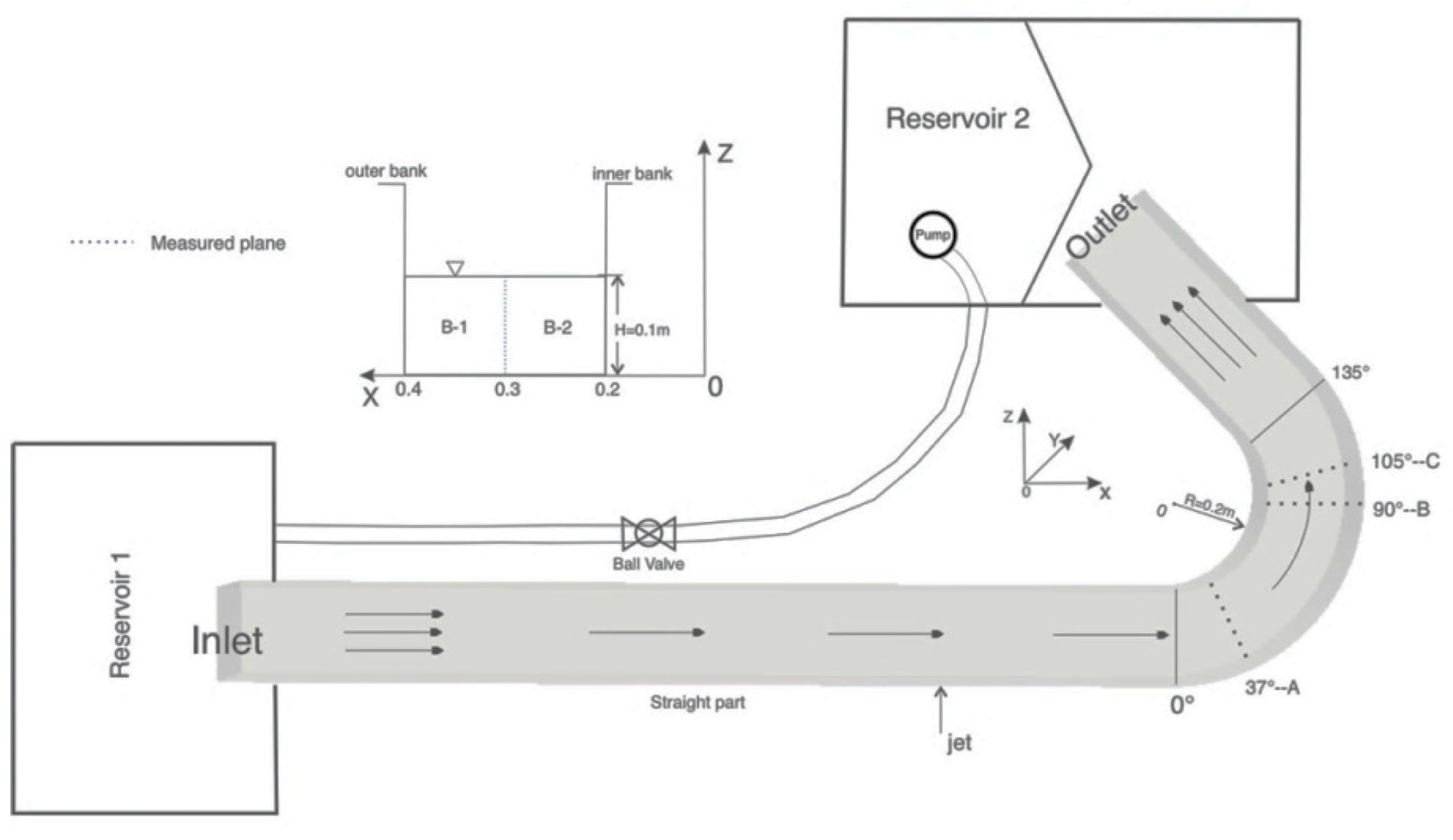
2.1. Laboratory Flume and Flow Properties

In this study, experiments were conducted to explore flow structures in a 135-degree bend flume with horizontal dense jets discharged into the straight section on the outer wall upstream of the bend. Three different density values were considered to investigate the influence of mixing behavior by dense jets on flow structures in the bend. A sketch of the experimental set-up, as well as the coordinate system, is given in Figure 1.

The flume was made of 1.27 cm thick clear acrylic, which ensured a good view of the flow both from the bottom and the sidewalls. The straight part of the flume in the inlet section was 2.2 m in length, and at the outlet side, the straight reach was approximately 0.55 m long. The straight reach at the inlet side was designed to be long enough to ensure the flow was fully developed before it entered the bend. The width and depth of the flume were both uniformly 0.2 m, and the centerline curvature radius (R_c) of this bend was 0.3 m. The current flume was classified as a strongly curved open channel bend due to Rc/b (b is the bend width) = 1.5; see Leschziner and Rodi [25]. At the entrance and the exit of the channel, two stainless steel reservoirs were set separately for water supply in the flume. A pump was placed in Reservoir #2 (Figure 1) to convey water to Reservoir #1 via a plastic pipe with an inner diameter of 12.7 cm. The flow rate in the flume was controlled by a ball valve near Reservoir #1, and a sharp crested weir was placed at the flume exit to adjust the water level in the channel. To measure the discharge with the flume, Reservoir #2 was divided into two components, between which a 90-degree V-notch weir was installed.

The jet nozzle was located at the straight upstream section of the bend entry section, about 55 cm away from the beginning of the bend, and it was set at the height of 4.5 cm to avoid boundary effects when the effluent was discharged. The length of the horizontal path of the jets was adequately long to ensure that they were well developed. In order to obtain a horizontal jet perpendicular to the main flow, a copper nozzle with an inner diameter of 0.95 cm was installed onto the outer bank of the bend wall at the above-mentioned location. Saline water was used as effluent in this study, and fresh tap water was used as the ambient receiving water body. The density of effluents was calculated according to the equation of state proposed by Millero and Poisson [26]. The equation was given as:

$$\rho ={\rho }_t+AS+B{S}^{3/2}+CS$$

(1)

where A $=8.24493\times {10}^{-1}-4.0899\times {10}^{-3}T+7.6438\times {10}^{-5}{T}^2-8.2467\times {10}^{-7}{T}^3+5.3875\times {10}^{-9}{T}^4$, B $=-5.72466\times {10}^{-3}+1.0227\times {10}^{-4}T-1.6546\times {10}^{-6}{T}^2$ and C $=4.8314\times {10}^{-4},$ and ${\rho }_t$ is the density of water that varies with the temperature, as follows:

$$\begin{array}{c}{\rho }_t=999.842594+6.793952\times {10}^{-2}T-9.095290\times {10}^{-3}{T}^2+\\ 1.001685\times {10}^{-4}{T}^3-1.120083\times {10}^{-6}{T}^4+6.536336\times {10}^{-9}{T}^5\end{array}$$

(2)

In the current study, salinity was set to 3.5, 10 and 16.5 to achieve the desired density difference. As the density of ambient water is lighter than that of the effluents, negatively buoyant jets were formed. A constant discharge rate was acquired by setting a constant head reservoir at an elevation of 85 cm above the flume bottom.

To better evaluate the cross-stream motion in the bend, a local coordinate system was used to define the measured planes as shown in Figure 1. Specifically, the origin was at the centerline of each cross-section, and the streamwise, span-wise, and vertical directions are denoted by s, n, and z correspondingly. Hence, the three time-averaged velocity components are u_s, u_n and u_z, indicating the velocities in the streamwise (longitudinal), span-wise (transverse) and vertical directions, respectively.

Hydraulic parameters were measured and collected in the straight channel at 0.55 m upstream of the bend entrance (

Table 1. Hydraulic characteristics of main flow in bend.

B (cm)	H (cm)	Rc (cm)	Q (L/s)	G (ms−2)	U (m/s)	Re	Fr
20	10	20	2	9.8	0.1	22024	0.22

B is the flume width; H is the flow depth; Rc is the centerline curvature radius; Q is the main flow discharge; g is the gravitational acceleration; the Reynolds number is calculated by Re = UH/ν; the Froude number is defined by Fr = U/(gH)^1/2.

). Each experimental measurement was taken until the flow was steady and uniform. The depth of the flow was 10 cm, with an averaged cross-sectional velocity of about 0.1 m/s. The water in the flume was replaced after every second measurement to ensure the ambient bend flow maintained low salinity.

2.2. Measurements and Procedure

Measurements of the velocity distribution were conducted using a Stereo-PIV system from LaVison, including the DaVis (Version 8.4) software for data acquisition and post processing. Measurements obtained with Stereo-PIV contained three velocity components (u₁, u₂ and u₃) over the two-dimensional (n-z) planes (two-dimensional three-components). All the measured surfaces were located in the bend section. Due to the current setup, 8 surfaces were measured, which yielded 4 cross-sectional planes (37°, 90°, 105° and 125°). Image planes were located in the n-z plane to collect the velocity distribution in three dimensions at the same time (Figure 2b).

The laser beam was fixed on a moveable cart under the flume and shot from below to avoid any possible reflection on the sidewall of the flume during the data recording session. The laser emission indicator was held with a three-prong extension clamp, then the clamp was fixed on the cast iron support ring stand. To meet the requirements of laser safety regulations, a canopy was built and placed on top of the flume to prevent laser light from propagating from the water’s surface. In addition, nine blocking boards covered by black, light absorbing material were arranged along the inner side of the flume to restrain the light scattering from the flume wall. Two cameras were placed horizontally at the outer bank side, towards the inner bank, at the same elevation as that of the calibration plate center (Figure 2c). The angle between the two cameras was set by trying to minimize the calibration evaluation value; hence, the angle was different for each measured plane.

A three-dimensional calibration target (two-level calibration plate from LaVision named #106-10), with white dots on both front and back sides, was chosen for scaling and calibrating. The calibration plate had dimensions of 10 × 10 cm; thus, each measured image plane occupied one half of the flume width, and two image planes were required to capture a channel section. In the present test, both sides of the calibration plate were used during the calibration (Figure 2d). The result of the calibration was then used in the mapping process, and a high-quality calibration generated an accurately mapped field of view. To diminish the influence of the deformation root from curvature during the mapping, a value used to evaluate calibration results was controlled at around 0.1. As for the focusing problem caused by the oblique view of cameras, Scheimpflug adapters were used to ensure that the field of view was uniformly focused. In addition, stereo self-calibration was engaged in order to minimize errors in the mapped image; see Prasad AK and Jensen K [27] for more references.

The illuminating components of the PIV system were two Nd-Yag pulsed laser beams (100 mJ per pulse at a wavelength of 532 nm), and the thickness of the optic sheet could be adjusted within a range from 3 to 5 mm. The flow was seeded with glass particles with a mean diameter of 20 μm and a density of 1.1 × 103 kg/m³. The required particle concentration is usually defined by the number of particles per pixel. The particle images were captured by two dual-frame sCMOS cameras with a frame rate of up to 50 Hz. The resolution of the cameras was 1028 × 2560 pixels with pixel size of 6.5 × 6.5 μm². The frequency of laser firing and the image capturing by the cameras were synchronized by a timing unit. In this study, sample pictures were taken with a corresponding time interval (3.7 ms) calculated depending on the flow velocity. Each measurement yielded a series of 1000 double-frame image pairs to be analyzed. The experimental method was verified by measuring velocity distribution in the straight section, where the flow structure was less complex. In the post-processing session, the sample image pairs were first manipulated by an image processing method such that quality improved pictures could be obtained for vector calculation interpreted using a multi-pass stereo cross-correlation algorithm. The size of the interrogation window decreased based on the number of pixels; the sizes of 64 × 64, 48 × 48 and 32 × 32 pixels were used for analysis. There was an overlap of 50% in the horizontal direction for 64 × 64 pixels, 25% circular overlap for 48 × 48 pixels, and 0% for 32 × 32 pixels. In addition, median filters were applied for image correcting and data restraining based on calculating flow averages and standard deviation.

In total, 8 surfaces were measured in this study, and measurements were made under steady, uniform flow conditions, as summarized in

Table 2. Table of experiments.

Slice #	Sjet	Smain	Ujet (m/s)	Umain (m/s)	Ρjet (kg/m3)	Δρ	Cross-Sectional Plane (Degree)
A (1 + 2)	3.5	0	0.2	0.1	1000	3	37
	10	0	0.2	0.1	1005	8	37
	16.5	0	0.2	0.1	1010	13	37
	-	0	-	0.1	-	-	37
B (1 + 2)	3.5	0	0.2	0.1	1000	3	90
	10	0	0.2	0.1	1005	8	90
	16.5	0	0.2	0.1	1010	13	90
	-	0	-	0.1	-	-	90
C (1 + 2)	3.5	0	0.2	0.1	1000	3	105
	10	0	0.2	0.1	1005	8	105
	16.5	0	0.2	0.1	1010	13	105
	-	0	-	0.1	-	-	105
D (1 + 2)	3.5	0	0.2	0.1	1000	3	125
	10	0	0.2	0.1	1005	8	125
	16.5	0	0.2	0.1	1010	13	125
	-	0	-	0.1	-	-	125

. To obtain a better calibration result for each section, the laser indicator and the cameras were circumspectly positioned with the same set-up as mentioned above. The velocity fields of four cross-sectional planes were generated, and extra measurements were also operated for repeatability validation. There were data fluctuations at the edge of each captured image plane, which resulted from the inevitable high intensity from the light source at the boundary. Thus, an uncertainty evaluation was performed to ensure data accuracy.

2.3. Analytical Methods

The measured data from the current PIV set-up yielded both the instantaneous three-dimensional velocity components and the averaged flow field at each measured section. The sampling frequency of the current PIV measurements was nearly 30 Hz. According to previous experimental studies, it can be conceived that such a frequency is below the frequency of the periodic motion and small-scale turbulence; see Graftieaux et al. [28]. Although the current sample size is insufficient in showing a correlation from the snapshots, it is capable of calculating the averaged velocity field. Therefore, an ensemble of averaged techniques was employed in extracting the averaged velocity and secondary circulation cells in the field of interest. The mean velocities ($u_s$,$u_n$,$u_z$) and fluctuating velocity components ($u_s^{\prime }$,$u_n^{\prime }$,$u_z^{\prime }$) were derived from the instantaneous velocities through the measured data. In this paper, mean flow and secondary flow quantities are evaluated with the averaged velocity.

The calculation of the vorticity is based on a MATLAB open-source code provided by Sebastian Endrikat [29]. The code detects the vortex in the s-axis through the n and z components of the velocity field and presents the location (x-y plane in the measurements), size and strength of every vortex identified.

3. Results and Analysis

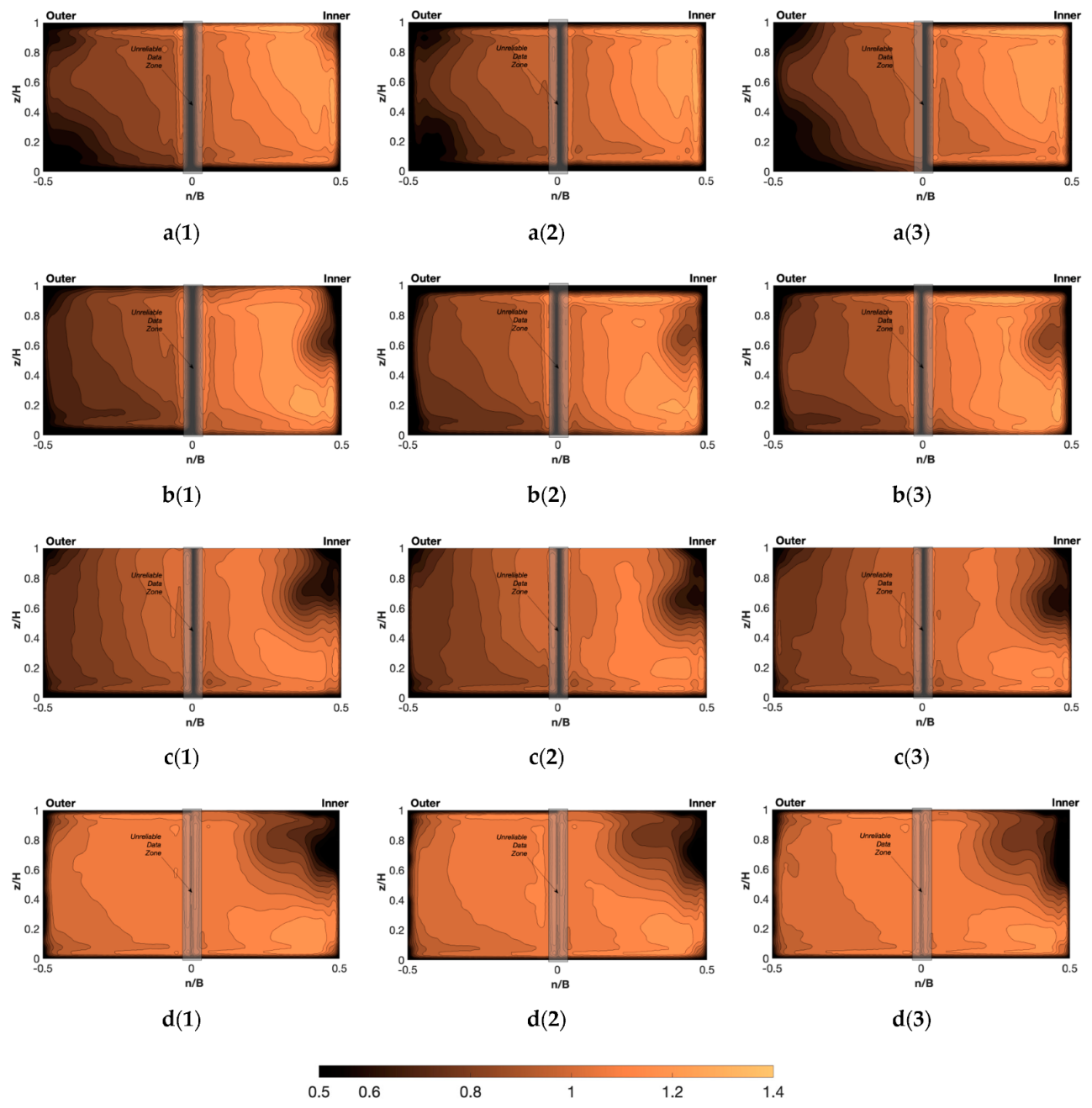
3.1. Mean Flow Patterns and Properties

Among all measured planes, the ones with lower uncertainty values (gathered directly from the DaVis) were selected for further investigation. All the contour profiles are smoothed using an interpolation method from MATLAB named Biharmonic (v4). Due to the current setup, two measured surfaces resulted for each cross-sectional plane. However, the streamwise velocity is the out-of-plane component; therefore, the streamwise velocity contour of all the cases at the outer bank side and inner bank side were computed separately for better analysis. Furthermore, it is acknowledged that the data acquired at the image edges using PIV technology were less accurate. Therefore, a 1 cm wide rectangular shadow was marked on the stitch line of the two images at one cross-sectional plane and named as unreliable data zone.

To better understand the mechanisms leading to velocity redistribution, the measured velocity field were normalized by the overall mean streamwise velocity U = Q/(BH) in the upstream straight channel. In non-dimensional coordinates, the inner wall and the outer wall are n/B = 0.5 and −n/B = −0.5 respectively and the water surface is at z/H = 1.

The averaged streamwise velocity distributions without the dense jets over the four measured cross-sections (37°, 90°, 105° and 125°) are presented in Figure 3, and the normalized streamwise velocity components of the flow with the incurrence of the jets, u_s/U (U = 0.1 m/s), are given in Figure 4. The highest value of u_s/U is around 1.4, implying that the velocity in the bend was redistributed and can go above the mean velocity in the straight channel. It can easily be noticed that the velocity magnitude at the outer bank side is increasing as the flow is approaching the bend exit (left side in Figure 3a–d). As expected, high momentum fluid was gradually transported from the inner side at the entrance to the outer bank near the exit; see Dietrich and Whiting [30]. As the flow proceeds through the bend, the contour interval of the streamwise velocity in the outer bank half becomes larger, which means that the velocity gradient is flattened as the flow exits the bend.

It can also be observed that, with the occurrence of negatively buoyant jets (Figure 4), the patterns of streamwise velocity distribution at the outer bank near the left bottom corner were slightly affected, and the region of the low velocity area expands towards the centerline as salinity increases. However, this phenomenon only presented at the beginning of the bend. In contrast, at the inner bank side, the influence on the velocity pattern caused by the negatively buoyant jets was mostly observed at the exit of the bend (e.g., 105 degrees and 125 degrees, Figure 4c,d), as opposed to the bend entrance. As shown in Figure 4d(1)–(3), there were low velocity regions near the inner bank at the upper half of the channel that were expected as the separation zones of bend flows, and the size of the low velocity core area are enlarged (deeper and wider) with an increase in salinity. This can indicate that the dense jets in the straight channel followed the main flow before entering the bend and were transported to the inner bank as the flow moved forward through the bend via secondary flow motion. The separation zone is not present at the bend entrance; it progressively develops in the bend. As shown in Figure 4a(2),(3), no separation zone was discovered, meaning that the formation of the separation zone can be postponed with higher salinity jets. Moreover, in the developed separation zones, the cores of these zones are dragged against the free surface as salinity increases (Figure 4a–c) for all the measured planes.

Further investigation of the qualitative analysis of the velocity profiles was described using the nondimensional maximum streamwise velocity (u_smax/U). Figure 5a exhibits the maximum streamwise velocity. As can be seen, for all cases, the maximum streamwise velocity slightly increases when the flow proceeds from 37 to 90 degrees, reaching the lowest value (among all the measured planes) at the 125-degree cross-sectional plane. The maximum streamwise velocity of the case without the jet shows the most similar trend as that of the jets with the largest salinity. It can be deduced that the maximum velocity magnitude in the bend is mostly dominated by the streamwise velocity, and the presence of the saline jets increase the maximum streamwise velocities in the bend.

The evolution of the maximum transverse and vertical velocity, however, presents partial similarities for different salinity conditions. As demonstrated in Figure 5b,c, the overall patterns of the evolution for both the maximum transverse velocity and vertical velocity are relatively consistent. Due to the presence of the negatively buoyant jets, the maximum transverse and vertical velocity were reduced by the jets at the beginning of the bend. When the flows are close to the bend exit, the maximum transverse and vertical velocity exceed the maximum values of the ones without jets. Figure 5d,e shows the location of the maximum streamwise velocity in the vertical direction and the spanwise direction respectively. As exhibited in the figures, within a measured plane, the negatively buoyant jets had little impact on the location of the maximum streamwise as flow proceeded the bend, however, the jets carried more influences on the maximum streamwise velocity in the vertical direction than that in the transverse direction. More precisely, the jets raised the elevation of where the maximum streamwise velocity was located, especially at the beginning and at the exit region of the bend.

The distribution of the normalized depth-averaged value of streamwise velocity component, u_s-depth/U, is given in Figure 6. Here, the core of the maximum depth-averaged streamwise velocity slowly moves to the outer bank, which also proves the transfer of high momentum fluids caused by the secondary flow. The saline jet appears to have little influence on the distribution of the depth-averaged streamwise velocity.

3.2. Cross-Sectional Flow Properties

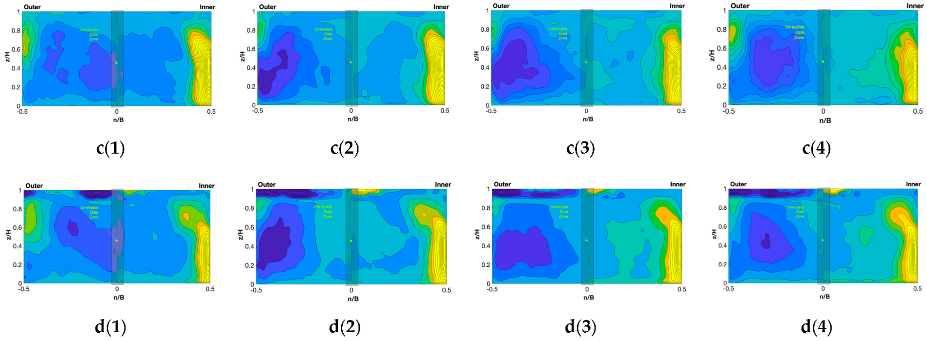
Figure 7 shows the distributions of the normalized transverse velocity; in the current setup, each cross-sectional plane was combined using two measurements taken at the outer bank side and the inner bank side, separately. As shown in Figure 7, the highest transverse velocities were observed in the deepest part of each cross-section at the channel bottom boundary. As expected, the fluids flow towards the inner bank at the bottom and towards the outer bank at the water surface, which forms a transverse flow also known as the helical flow. As previously shown in the distribution of the streamwise velocity, the dense jets influence the transverse flow at the lower outer corner of the bend entrance. At the 37-degree plane (Figure 7a(2)–(4)), the transition area between the inward velocity and the outward velocity region in the lower part of the outer bank side of the cross-sectional plane is enlarged by the jets. As salinity increases, the core of the positive transverse velocity region shrinks in the vertical direction, attenuating the transit of the fluids that go towards the inner bank at the lower part of the cross-section. This phenomenon can also be observed at the rest of the measured planes (Figure 7b–d). Figure 7b(1) shows a velocity increase close to the water’s surface, and this high velocity region (in dark blue) gradually moves to the outer bank as the flow continues in the bend (Figure 7c(1),d(1)). With the occurrence of jets, the transport of the high velocity region to the outer bank of the bend is accelerated at the water surface.

In the left and the right upper corners of each cross section, there are fluids moving in the opposite direction as the ambient flow. According to the location of the regions, they are called the outer bank circulation zone and inner bank separation zone respectively. Unlike the streamwise velocity components, the size of the inner bank zone decreases as salinity increases at each cross-section, while the outer bank zone first decreases and then increases with the increasing salinity (Figure 7a–d).

Figure 8 demonstrates all the dimensionless vertical velocity distributions of all the measured planes. It has been proven by many researchers that the fluids in the bend follow an upward path near the inner bank and go downward at the outer bank. This pattern is also well captured by the current measurements. Moreover, the size of the inner side upward flow region in the beginning of the bend is larger than that of the subsequent downstream cross-sections (Figure 8a,b). Specifically, the tops of these upward flow regions are found to be slightly stretched and bent towards the centerline, which implies the existence of the separation zone (Figure 8b–d).

A large downward velocity region at the lower outer bank is noticed in Figure 8a(1), but it disappears as the flow continues in the bend (Figure 8b(1)–d(1)). When there are negatively buoyant jets present, this region persists throughout the bend. This agrees well with the variation of the maximum vertical velocity (Figure 5c), i.e., at the beginning of the bend, the maximum vertical velocity with dense jets is smaller than that of the one without jets. Furthermore, as shown in Figure 8a, the core of this downward velocity region is slightly lifted as the salinity increases. The same as the influence on streamwise velocity caused by the jets in the outer bank, this phenomenon is only observed at 37-degrees. For the rest of the measured cross-sections, the core of the high downward velocity region was attenuated with increasing salinity (Figure 8b(2)–(4)). This attenuation was found to roughly continue through the bend at 105 and 125 degrees. As presented in Figure 8, at the outer bank side, immediately below the water surface, an opposite upward velocity region was also found. The same as the trend of the transverse velocity, a gradual decrease in the size of this specific region was observed, followed by an increase with the rising jet salinity.

3.3. Secondary Flow

For most of the measured cases, typical vortices of bend flows, such as the outer bank cell and the main center cell, are visible in the experiments, and the separation zone at the inner bank is captured at certain degrees. Specifically, the large primary secondary flow also known as the center region cell located in the lower center of the channel and a counter-rotating small cell that normally can be found at the outer bank below the water’s surface. Such results have been observed in previous studies, e.g., Rozovskii, de Vriend, and Blanckaert et al. [1,4,31]. The primary center region cell has been known to be the result of the local imbalance between the centrifugal force and the cross-stream pressure gradient, and turbulence has little contribution to generating the center region cell. Unlike the center region cell, turbulence plays an important role in the formation of the outer bank cell, but it is not the exclusive reason. Vortex skewing, which results from centrifugal force, is also conducive to the outer bank cell [4]. At cross-sections of 90°, 105°, and 125°, the core of the center region cell in each plane shifts to the inner bank compared to the 37°, and it stays at the inner bank until it exits the bend. This result is also found to be consistent with existing research results, e.g., Blanckaert and Graf [15], Abhari et al. [32], and Bai et al. [33].

To better understand the influence of negatively buoyant jets, the sizes and vorticities of the secondary flow are calculated using an online open-source code called IDvortex [29] developed in MATLAB. Figure 9 shows both the outer bank cell and the center region cell variation with the presence of the jets. The evolution of the center region cell is consistent for cases in which the salinity values were 3.5 and 10, e.g., the size of the center region cell experienced a decreasing trend, followed by an increase and another decrease as flow proceeded in the bend. However, as for the densest jet case, at the beginning of the bend, the size of the center region cell would continue increasing, and the same trend can be obtained for the no jet case (Figure 9a). According to the plots, the maximum difference between the cases with and without the jet was found at 37 degrees, which is located at the beginning of the bend. Moreover, the difference of the center region cell size between the first and the last cross-sectional plane measured in the bend decreases as the salinity increases. On the contrary, the variation in the outer bank cell size with the salinity had an opposite trend. Meanwhile, the size of the outer bank cell was decreased with the presence of the negatively buoyant jets. However, when the flow approached the exit of the bend, the size of the outer bank cell with the jets maintained a descending trend rather than a rising tendency (Figure 9b). Analogously, the strength of the outer bank cell with the occurrence of the jets was lower than the one without the jets, while the evolution for both the size and the intensity of the center region cell with the jets shows more variation (Figure 9a,c). The reason behind the variation might be the different driving mechanisms for the generation of these two types of cells. The center region cell is regarded to result from centrifugal force rather than from turbulence; hence, the jet-induced turbulence cannot be applied directly to it. The effects on the center region cell could be attributed to the transport of the jet-induced momentum, and the mixing behavior itself also influences the momentum distribution in the bend. Consequently, this process deforms the downstream velocity profile, which changes the centrifugal force. As for the outer bank cell, although few examinations have been revealed for the underlying mechanisms, the hypothesis that the outer-bank cell is formed by the combined exertion of the centrifugal force and turbulence has been widely accepted [4]. Therefore, the presence of turbulent jets can act directly on the turbulence in the bend flow. However, the reduction in the size and strength of the outer bank cell indicates that the jets incurred additional turbulence stress, which favors the dissipation of the outer bank vorticity.

4. Conclusions

The present study examined mixing of a negatively buoyant effluent jet in a 135-degree open channel bend. High-quality three-dimensional velocities were measured throughout four channel cross-sections using a stereo-PIV system. The experiments were designed to investigate the influences on the 3D flow field caused by the negatively buoyant jet in the bend flow. Jets with three different salinities were investigated, as well as a case without a jet. The observations focused on the streamwise and cross-stream velocity distribution, the maximum velocity, and the secondary flow properties. The main conclusions may be summarized as follows:

Multiple flow patterns were captured in different bend cross-sections, i.e., the curvature-induced helical flow, the outer bank counter-rotating cell, and the inner bank separation zone.

The negatively buoyant jets have little impact on the maximum streamwise velocities evolution within the bend as well as the depth-averaged streamwise velocities; however, the maximum transverse and vertical velocity of the flow varies with salinity, especially in the vertical direction. More specifically, the outer bank downward velocity was interrupted by the jets and decreased as salinity increased.

The influence of the jets on the center region cell vorticity was mostly observable at the beginning and exit of the bend, where the mixing process started and the secondary decayed, respectively. This can be attributed to the sudden change of flow complexity near the entry and exit of the bend. The failure to obtain a continuous variation on the secondary flow with respect to the increase in salinity is due to the distinctive transport and mixing behavior of the dense jets in a bend.

The jet-induced turbulence stress favors the dissipation of the outer bank vorticity, although at different cross-sections, this attenuation varies.

References

1. Rozovskii, I.L. Flow of Water in Bends of Open Channels; Israel Program for Scientific Translations, Translator; Academy of Sciences of the Ukrainian SSR: Kyiv, Ukraine, 1957; p. 233. (In Russian) [Google Scholar]
2. Engelund, F.; Skovgaard, O. On the origin of meandering and braiding in alluvial streams. J. Fluid Mech. 1973, 57, 289–302. [Google Scholar] [CrossRef]
3. Struiksma, N.; Olesen, K.W.; Flokstra, C.; De Vriend, H.J. Bed deformation in curved alluvial channels. J. Hydraul. Res. 1985, 23, 57–79. [Google Scholar] [CrossRef]
4. Blanckaert, K.; De Vriend, H.J. Secondary flow in sharp open-channel bends. J. Fluid Mech. 2004, 498, 353–380. [Google Scholar] [CrossRef] [Green Version]
5. Blanckaert, K.; de Vriend, H.J. Nonlinear modeling of mean flow redistribution in curved open channels: Nonlinear modeling of mean flow. Water Resour. Res. 2003, 39, 1375. [Google Scholar] [CrossRef]
6. Thompson, J. On the origin of the windings of rivers in alluvial plains, with remarks on the flow of water in pipes. Royal Soc. Lond. Proc. 1876, 25, 5–8. [Google Scholar]
7. Shukry, A. Flow around bends in an open flume. Trans. ASCE 1950, 115, 751–779. [Google Scholar] [CrossRef]
8. Naot, D.; Rodi, W. Calculation of secondary currents in channel flow. J. Hydraul. Eng. 1982, 108, 948–968. [Google Scholar] [CrossRef]
9. Odgaard, A.J.; Bergs, M.A. Flow processes in a curved alluvial channel. Water Resour. Res. 1988, 24, 45–56. [Google Scholar] [CrossRef]
10. Rhoads, B.L.; Welford, M.R. Initiation of river meandering. Prog. Phys. Geogr. 1991, 15, 27–156. [Google Scholar] [CrossRef]
11. Whiting, P.J.; Dietrich, W.E. Experimental studies of bed topography and flow patterns in large amplitude meanders: 1. Observations. Water Resour. Res. 1993, 9, 3605–3614. [Google Scholar] [CrossRef]
12. Kawai, S.; Julien, P.Y. Point bar deposits in narrow sharp bends. J. Hydraul. Res. 1996, 34, 205–218. [Google Scholar] [CrossRef]
13. Gholami, A.; Akhtari, A.A.; Minatour, Y.; Bonakdari, H.; Javadi, A.A. Experimental and numerical study on velocity fields and water surface profile in a strongly-curved 90° open channel bend. Eng. Appl. Comput. Fluid Mech. 2014, 8, 447–461. [Google Scholar] [CrossRef] [Green Version]
14. Doneker, R.L.; Jirka, G.H. Expert Systems for Design and Mixing Zone Analysis of Aqueous Pollutant Discharges. J. Water Resour. Plan. Manag. 1991, 117, 679–697. [Google Scholar] [CrossRef]
15. Blanckaert, K.; Graf, W.H. Experiments on flow in a strongly curved channel bend. In Proceedings of the 29th Congress-International Association for Hydraulic Research, Beijing, China, 16–21 September 2001. [Google Scholar]
16. Termini, D.; Piraino, M. Experimental analysis of cross-sectional flow motion in a large amplitude meandering bend. Earth Surf. Process. Landf. 2010, 36, 244–256. [Google Scholar] [CrossRef]
17. Vaghefi, M.; Akbari, M.; Fiouz, A.R. An experimental study of mean and turbulent flow in a 180-degree sharp open channel bend: Secondary flow and bed shear stress. KSCE J. Civ. Eng. 2016, 20, 1582–1593. [Google Scholar] [CrossRef]
18. Wei, M.; Blanckaert, K.; Heyman, J.; Li, D.; Schleiss, A.J. A parametrical study on secondary flow in sharp open-channel bends: Experiments and theoretical modelling. J. Hydro-Environ. Res. 2016, 13, 1–13. [Google Scholar] [CrossRef]
19. Blanckaert, K. Saturation of curvature-induced secondary flow, energy losses, and turbulence in sharp open channel bends: Laboratory experiments, analysis, and modeling. J. Geophys. Res. 2009, 114, F03015. [Google Scholar] [CrossRef] [Green Version]
20. Kikkert, G.A.; Davidson, M.J.; Nokes, R.I. Inclined Negatively Buoyant Discharges. J. Hydraul. Eng. 2007, 133, 545–554. [Google Scholar] [CrossRef]
21. Oliver, C.J.; Davidson, M.J.; Nokes, R.I. Removing the boundary influence on negatively buoyant jets. Environ. Fluid Mech. 2013, 13, 625–648. [Google Scholar] [CrossRef]
22. Zhang, S.; Jiang, B.; Law, A.W.K.; Zhao, B. Large eddy simulations of 45° inclined dense jets. Environ. Fluid Mech. 2016, 16, 101–121. [Google Scholar] [CrossRef]
23. Choi, K.W.; Lai Chris, C.K.; Lee Joseph, H.W. Mixing in the Intermediate Field of Dense Jets in Cross Currents. J. Hydraul. Eng. 2016, 142, 04015041. [Google Scholar] [CrossRef]
24. Schreiner, H.K.; Rennie, C.D.; Mohammadian, A. Trajectory of a jet in cross-flow in a channel bend. Environ. Fluid Mech. 2018, 18, 1301–1319. [Google Scholar] [CrossRef]
25. Leschziner, M.A.; Rodi, W. Calculation of strongly curved open channel flow. J. Hydraul. Div. 1979, 105, 1297–1314. [Google Scholar] [CrossRef]
26. Millero, F.J.; Poisson, A. International one-atmosphere equation of state of sea water. J. Deep-Sea Res. 1981, 28, 625–629. [Google Scholar] [CrossRef]
27. Prasad, A.K.; Jensen, K. Scheimpflug stereo camera for particle image velocimetry in liquid flows. Appl. Opt. 1995, 34, 7092–7099. [Google Scholar] [CrossRef]
28. Graftieaux, L.; Michard, M.; Grosjean, N. Combining PIV, POD and vortex identification algorithms for the study of unsteady turbulent swirling flows. Meas. Sci. Technol. 2001, 12, 1422–1429. [Google Scholar] [CrossRef]
29. Endrikat, S. Find Vortices in Velocity Fields. MATLAB Central File Exchange. Available online: https://www.mathworks.com/matlabcentral/fileexchange/52343-find-vortices-in-velocity-fields (accessed on 28 April 2022).
30. Dietrich, W.E.; Whiting, P.J. Boundary shear stress and sediment transport in river meanders of sand and gravel. In River Meandering; Ikeda, S., Parker, G., Eds.; AGU: Washington DC, USA, 1989; Volume 12, pp. 1–50. [Google Scholar]
31. Blanckaert, K.; Duarte, A.; Chen, Q.; Schleiss, A.J. Flow processes near smooth and rough (concave) outer banks in curved open channels. J. Geophys. Res. Earth Surf. 2012, 117, F04020. [Google Scholar] [CrossRef] [Green Version]
32. Abhari, M.N.; Ghodsian, M.; Vaghefi, M.; Panahpur, N. Experimental and numerical simulation of flow in a 90 bend. Flow Meas. Instrum. 2010, 21, 292–298. [Google Scholar] [CrossRef]
33. Bai, R.; Zhu, D.; Chen, H.; Li, D. Laboratory Study of Secondary Flow in an Open Channel Bend by Using PIV. Water 2019, 11, 659. [Google Scholar] [CrossRef] [Green Version]
Figure 1. Sketch of the bend flume and the coordinate system with the flow condition in the flume.
Water 14 01898 g001
Figure 2. PIV setup with a laser and a camera: (a) sketch of the bend with the coordinate system (b) n-z plane of the coordinate system; (c) camera layout; (d) configuration for the PIV experiments. (the blue boxes are the cameras, the white box is the laser emitter, and the green sheet represents the laser light beam).
Water 14 01898 g002
Figure 3. Streamwise velocity of the measured cross-sections without the jets: (a) 37 degrees, (b) 90 degrees; (c) 105 degrees; (d) 125 degrees.
Water 14 01898 g003
Figure 4. Streamwise velocity distribution at the measured cross-sections: (a) 37 degrees; (b) 90 degrees; (c) 105 degrees; (d) 125 degrees. The numbers 1, 2, and 3 denote different jet conditions (1) S = 3.5; (2) S = 10; (3) S = 16.5.
Water 14 01898 g004
Figure 5. Dimensionless maximum velocities proceed at the bend with different jet conditions: (a) streamwise velocity; (b) transverse velocity; (c) vertical velocity; (d) evolution of the maximum streamwise velocity in the vertical direction; (e) evolution of the maximum streamwise velocity in the transverse direction.
Water 14 01898 g005aWater 14 01898 g005b
Figure 6. Dimensionless depth-averaged streamwise velocity across each sectional plane, with different jet conditions: (a) 37-degree plane; (b) 90-degree plane; (c) 105-degree plane; (d) 125-degree plane.
Water 14 01898 g006
Figure 7. Dimensionless transverse velocity distribution at (a) 37 degrees; (b) 90 degrees; (c) 105 degrees; (d) 125 degrees. The numbers 1, 2, 3, and 4 denote different jet conditions (1) no jet; (2) S = 3.5; (3) S = 10; (4) S = 16.5.
Water 14 01898 g007aWater 14 01898 g007b
Figure 8. Dimensionless vertical velocity distribution at (a) 37 degrees; (b) 90 degrees; (c) 105 degrees; (d) 125 degrees. The numbers 1, 2, 3, and 4 denote different jet conditions (1) no jet; (2) S = 3.5; (3) S = 10; (4) S = 16.5.
Water 14 01898 g008aWater 14 01898 g008b
Figure 9. Secondary flow property evolution with respect to jet salinity in the bend: (a) center region; cell size; (b) outer bank cell size; (c) center region cell vorticity; (d) outer bank cell vorticity.
Water 14 01898 g009