Comparison of Numerical Methods in Simulating Lake–Groundwater Interactions: Lake Hampen, Western Denmark

Abstract

The numerical simulation of lake–groundwater interaction dynamics is very challenging, and, thus, only few model codes are available. The present study investigated the performance of a new method, namely, the Sloping Lakebed Method (SLM), in comparison to the widely used MODFLOW lake package (LAK3). Coupled lake–groundwater models based on LAK3 and SLM were developed for Lake Hampen, Denmark. The results showed that both methods had essentially the same accuracy when simulating the lake water level, the groundwater head and the overall water balance. The SLM-based model had the potential to reproduce the change of the lake surface area in a more natural way. Moreover, the vertical discretization of a lake in the SLM is independent of the groundwater model, and, thus, the model grid at the top layers could be considerably coarsened without a loss of model accuracy. This could lead to savings in computational time of approximately 30%.

1. Introduction

The hydraulic connection between lakes and groundwater is an important factor to consider in numerical simulations of the hydrological cycle, because a change in water quantity and/or quality in one system will inevitably impact the other [1,2,3,4,5]. Understanding the interactions between lakes and the underlying groundwater system is therefore essential for effective water resources management [6,7,8,9,10].

The observation of lake–groundwater interactions can be obtained through field measurements using, for instance, seepage meters [11,12,13], stable isotope sampling [14,15] and hydraulic gradient measurements based on piezometers or potentiometers [16,17]. However, these methods mainly yield point data of local fluxes, which, in many cases, are difficult to upscale to the entire lake due to spatial heterogeneity. This issue may partly be addressed by applying temperature-based mapping methods, which allow for high spatial resolution [18]. Complementary to field measurement, distributed hydrological models that integrate information across different temporal and spatial scales are commonly used for estimating lake–groundwater interactions and can thus be used to address the impact of human and/or climate forcing on the water circulation [19,20,21,22,23,24].

The lake package in the MODFLOW family is one of the most widely used numerical codes for simulating lake–groundwater interactions [25,26]. It provides a separate water budget for the lake, enabling it to estimate not only the fluctuating lake water stage but also the volumetric water exchange between a lake and an aquifer [27,28]. However, even the most up-to-date lake package in MODFLOW, LAK3, has certain limitations. In order to represent the lake bathymetry in more detail, the upper part of the groundwater model, where the lake resides, has to be divided into numerous thin layers [29]. As a result, the computational time is considerably increased, and, in some cases, it could lead to non-convergence.

To overcome this problem, a new model code for simulating lake–groundwater interaction was developed, namely, the Sloped Lakebed Method (SLM) [30]. One of the most distinctive features of the SLM is that the bathymetrical representation of the lake bottom is independent of the discretization of the groundwater model. In the published studies, the SLM code is introduced, several test simulations are performed under steady-state flow conditions and the model results are compared with those of the corresponding LAK3 code [30]. The present study is our first attempt to simulate lake–groundwater interaction under transient flow conditions using the SLM. In this manuscript, we propose the comparison of the new SLM with the classic LAK3 code so that their ability to simulate water movement and storage, especially the computational time efficiency in these simulations, can be objectively investigated.

The study site of the comparison is Lake Hampen, located in western Denmark. The lake is groundwater-dominated and thus very suitable for studying lake–groundwater interactions. The observed data from groundwater boreholes and lake gages are readily available. Moreover, a model has been previously set up in MODFLOW with the LAK3 package [16], which can be used as a benchmark in the present study.

2. Materials and Methods

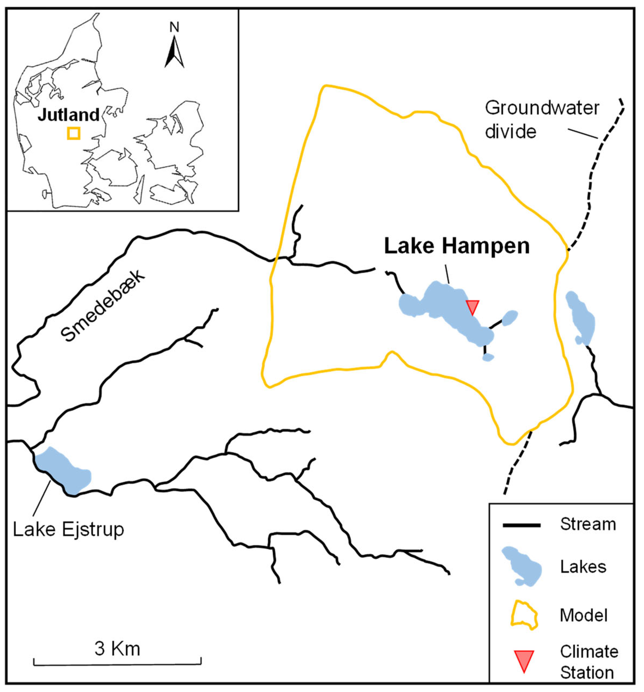
2.1. Study Area

Lake Hampen is located in the middle of the Jutland Peninsula in western Denmark (Figure 1). The lake has a surface area of approximately 0.76 km², on average, and is constituted by a shallow basin to the west (maximum depth of 2 m) and a deep basin to the east (maximum depth of 13 m). The land cover near the lake primarily consists of forests and grass fields, with nearly no urban areas.

The lithological boreholes around the lake show that the hydraulic conductivity of the aquifer is slightly higher in the east than in the west. The lake bottom sediment mainly consists of fine-grained organic materials in the deeper parts of the lake to the east and a peat layer throughout the shallow part of the lake to the west. The average precipitation measured at a climate station near the lake shows 888 mm/yr in the period between 1970 and 2007. In 2008, the annual precipitation was 901 mm, the calculated potential evaporation was 407 mm and the average lake level was 79.06 m.a.s.l. Further details regarding the regional geology can be found in Kidmose et al. (2011) [16].

2.2. Methods and Data

The numerical simulations of lake–groundwater interactions are compared between: (a) MODFLOW coupled with the LAK3 package [27,28] and (b) MODFLOW coupled with the new Sloped Lakebed Method (SLM) developed by Lu et al. (2020) [30].

2.2.1. The LAK3 Method

LAK3 is a lake package commonly used in connection with MODFLOW [21,28]. It is used to simulate interactions between lakes and the surrounding aquifers and is a result of several significant updates from previous lake packages (LAK1 and LAK2). In LAK3, the extent of the lake is represented by inactive cells, and the active cells bordering the inactive space represent the adjacent aquifer. The volumetric water exchange between the lake and the aquifer is calculated by Darcy’s Law based on the hydraulic head difference between them [28]. LAK3 has a separate lake water budget, enabling it to estimate not only the seepage loss and gain of the aquifer but also the fluctuating lake water stage. The lake status in LAK3 is simulated and updated at each time step using the following water budget equation:

$$h_l^n=h_l^{n-1}+\mathsf{\Delta }t\frac{P-E+Rnf-W-sp+Q_{si}-Q_{so}}{A_s}$$

(1)

where $h_l^n$ and $h_l^{n-1}$ are the lake water levels at the present and previous time steps (m); $\mathsf{\Delta }t$ is the length of the time step (s); $P$ is the inflow from precipitation over the lake surface (m³/s); $E$ is the outflow from evaporation over the lake surface (m³/s);$Rnf$ is the discharge into the lake from the infiltration excessive surface runoff (m³/s);$W$ is the outflow due to lake water withdrawals, where negative values represent net (anthropogenic) inflows (m³/s);$sp$ is the net flow from seepage between the lake and the aquifer during the time step, where positive values indicate seepage from the lake into the aquifer (m³/s); $Q_{si}$ is the inflow from the upstream (m³/s); $Q_{so}$ is the outlet discharge of the lake to the downstream (m³/s); $A_s$ is the surface area of the lake at the beginning of the time step (m²).

It is worth noting that the lakebed elevation is characterized by the bottom elevation of inactivated aquifer grid cells in LAK3. Therefore, adequate representations of lake bottom geometries require relatively many vertical model layers to be created (Figure 2).

2.2.2. The SLM Method

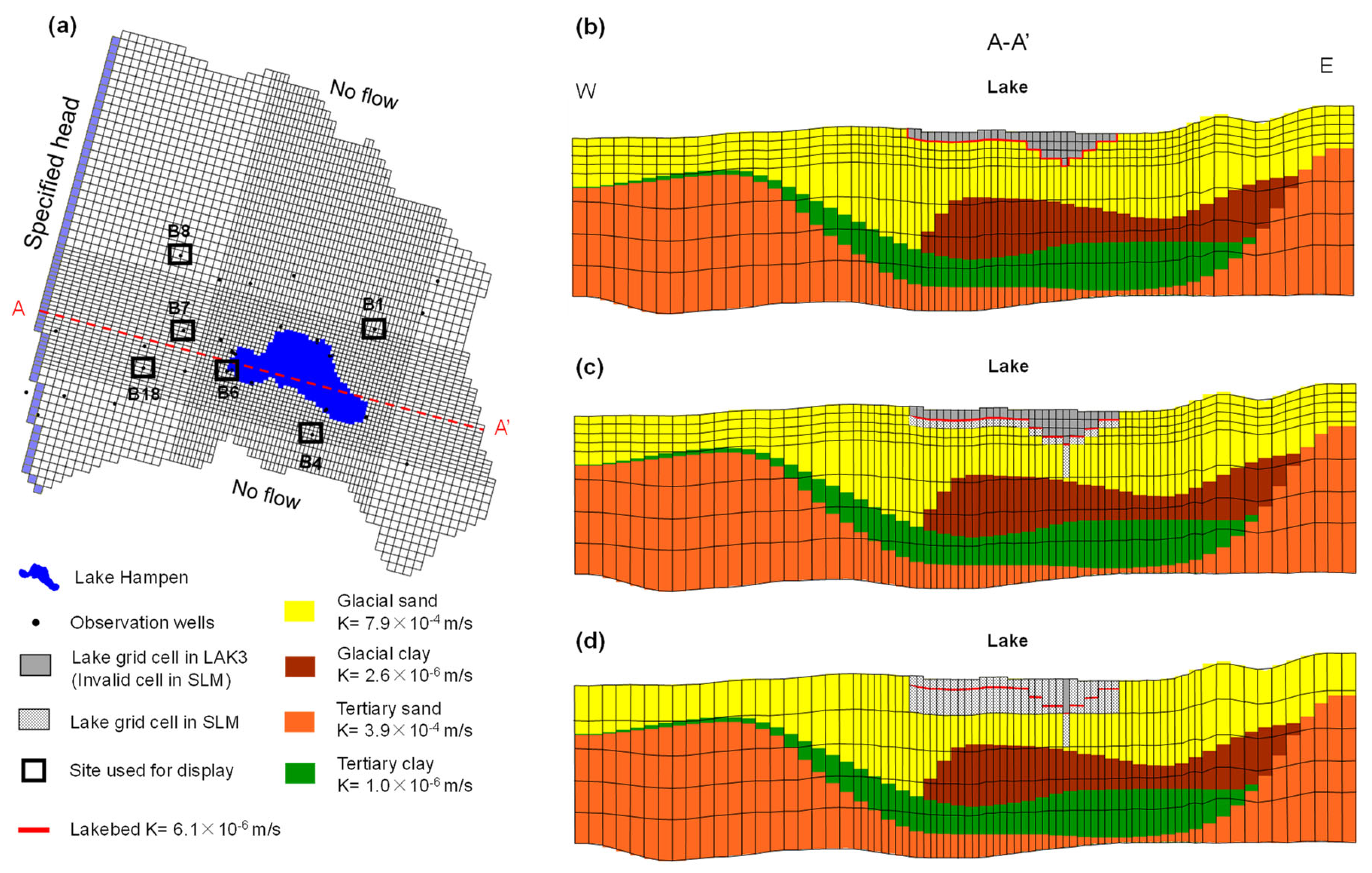
The SLM builds upon the numerical groundwater model MODFLOW. In the SLM, the maximum extent of the lake area is divided into a submerged area which is currently under water and an unsubmerged area which is currently above the lake water level (Figure 2a,b):

$$A_T=A_{UA}\left(h_l\right)+A_{SA}\left(h_l\right)$$

(2)

where $A_T$ is the total area of the lake, which is constant during the simulation (m²);$h_l$ is the lake water level (m); $A_{UA}\left(h_l\right)$ and $A_{SA}\left(h_l\right)$ are the unsubmerged area and submerged area, respectively (m²), which will change as the lake stage changes. The lake water budget is formulated in Equation (3), and each term is explained in Equations (4)–(10):

$$V^n\left(h_l^n\right)=V^{n-1}\left(h_l^{n-1}\right)+\mathsf{\Delta }t\left(P+Rnf+Q_{si}+G_p^{in}+G_N^{in}\right)-\mathsf{\Delta }t\left(E+W+G_p^{out}+Q_{so}\right)$$

(3)

$$P=p·A_{SA}\left(h_l^{n-1}\right)$$

(4)

$$Rnf=p·\gamma ·A_{UA}\left(h_l^{n-1}\right)$$

(5)

$$E=e_0·A_{SA}\left(h_l^{n-1}\right)$$

(6)

$$G_p^{in}=C_m·\left(h_{gw}-h_l^{n-1}\right)$$

(7)

$$G_N^{in}=C_m·\left(h_{gw}-h_{bot}\right)$$

(8)

$$G_p^{out}=C_m·\left(h_l^{n-1}-h_{gw}\right)$$

(9)

$$Q_{so}=m{B}_0\sqrt{2g}{h_l^{n-1}}^{3/2}$$

(10)

where $V^n\left(h_l^n\right)$ and $V^{n-1}\left(h_l^{n-1}\right)$ are the lake water volumes at the end and beginning of the time step (m³);$h_l^n$ and $h_l^{n-1}$ are the lake water levels at the end and beginning of the time step (m);$h_{gw}$ is the groundwater level (m);$h_{bot}$ is the elevation of the lake bottom (m); $\mathsf{\Delta }t$ is the length of the time step (s); $P$ is the inflow from precipitation over the submerged area (m³/s); $p$ is the precipitation intensity (m/s); $Rnf$ is the inflow from surface water runoff over the unsubmerged area (m³/s); $\gamma$ is the runoff coefficient (unitless); $Q_{si}$ is the inflow from upstream rivers (m³/s); $G_p^{in}$ is the groundwater inflow from the aquifer to the submerged area (m³/s);$C_m$ is the hydraulic conductance of the lakebed–aquifer interface (m²/s); $G_N^{in}$ is the outflow to the submerged area of groundwater locally created in the unsubmerged area (m³/s);$E$ is the flow from evaporation over the submerged area (m³/s); $e_0$ is the evaporation rate (m/s);$W$ is the outflow due to lake water withdrawals (m³/s); $G_p^{out}$ is the outflow from the submerged area into the aquifer (m³/s);$Q_{so}$ is the outlet discharge of the lake through the downstream channel (m³/s);$m$ is the discharge coefficient (unitless); $B_0$ is the channel width (m); $g$ is the acceleration of gravity (m/s²).

The lake water balance equation under transient flow conditions can be solved with an iterative algorithm. The average submerged area, which is calculated using the average lake water level, was used to calculate each term in the equation. The calculated average lake water level in the nth iteration, $\overline{h_l}$, is found to be

$$\overline{h_l}=\left(1-\eta \right)h_l^{n-1}+\eta h_l^n$$

(11)

where $\eta$ is the weight factor, and its value ranges from 0 to 1.

The grid cells where the lakebed exists are denoted as lakebed cells in the SLM, and the cells above it are defined as invalid cells (Figure 2d). This makes the bathymetrical representation of lake bottoms independent of the horizontal discretization of the groundwater domain in the SLM method. The SLM method assumes that the lakebed within the lakebed cells is sloped (Figure 2d). Further details regarding the SLM method can be found in Lu et al. (2020) [30].

2.2.3. Model Setup

Transient flow models were developed for Lake Hampen and its surrounding aquifer using LAK3 and the SLM as the lake package, each coupled with MODFLOW as the groundwater flow model. The northern, eastern and southern model boundary was defined by the groundwater divide, so the no-flow boundaries were defined in the north, east and south borders (Figure 3a). The western border of the model domain was defined as the general head boundary using the interpolated averaged head values from nearby wells measured throughout 2008. The geology was represented by five hydrogeologic units, namely, glacial sand, glacial clay, tertiary clay, tertiary sand and lake bottom sediments (Figure 3b–d). Four groundwater recharge zones were specified based on the unsaturated zone thickness and land use (Figure 4). The recharge values for the four different zones were calculated by HYDRUS-1D.

A steady-state model using LAK3 was used in a previous study to calibrate against 32 hydraulic head observations and 1 lake-level observation [16]. The resulted hydraulic conductivity values (K values in Figure 3) of the different hydrogeological units were used in all models in the present study under transient flow conditions. The models were simulated from 10 December 2003 to 7 January 2012, with a stress period every 10 days. The year 2008 was used for model validation.

The top part of the SLM-based models was delineated into four layers (SLM-TS4) and one layer (SLM-TS1). The four-layer model had a setup consistent with what was used in Kidmose et al. (2011) [16], which was denoted as LAK3-TS4. The one-layer models merged the top four layers into one, as seen in Figure 3d. The horizontal discretization (i.e., along the x- and y-axes) are the same for all models, with a base-grid of 100 × 100 m cells and locally refined to 50 × 50 m when near the lake (Figure 3a). The model domain was divided into 72 rows and 84 columns, with 4589 valid grid cells in a single layer. More details about the numerical MODFLOW model for Lake Hampen and its catchment can be found in Kidmose et al. (2011, 2015) [6,16].

3. Results

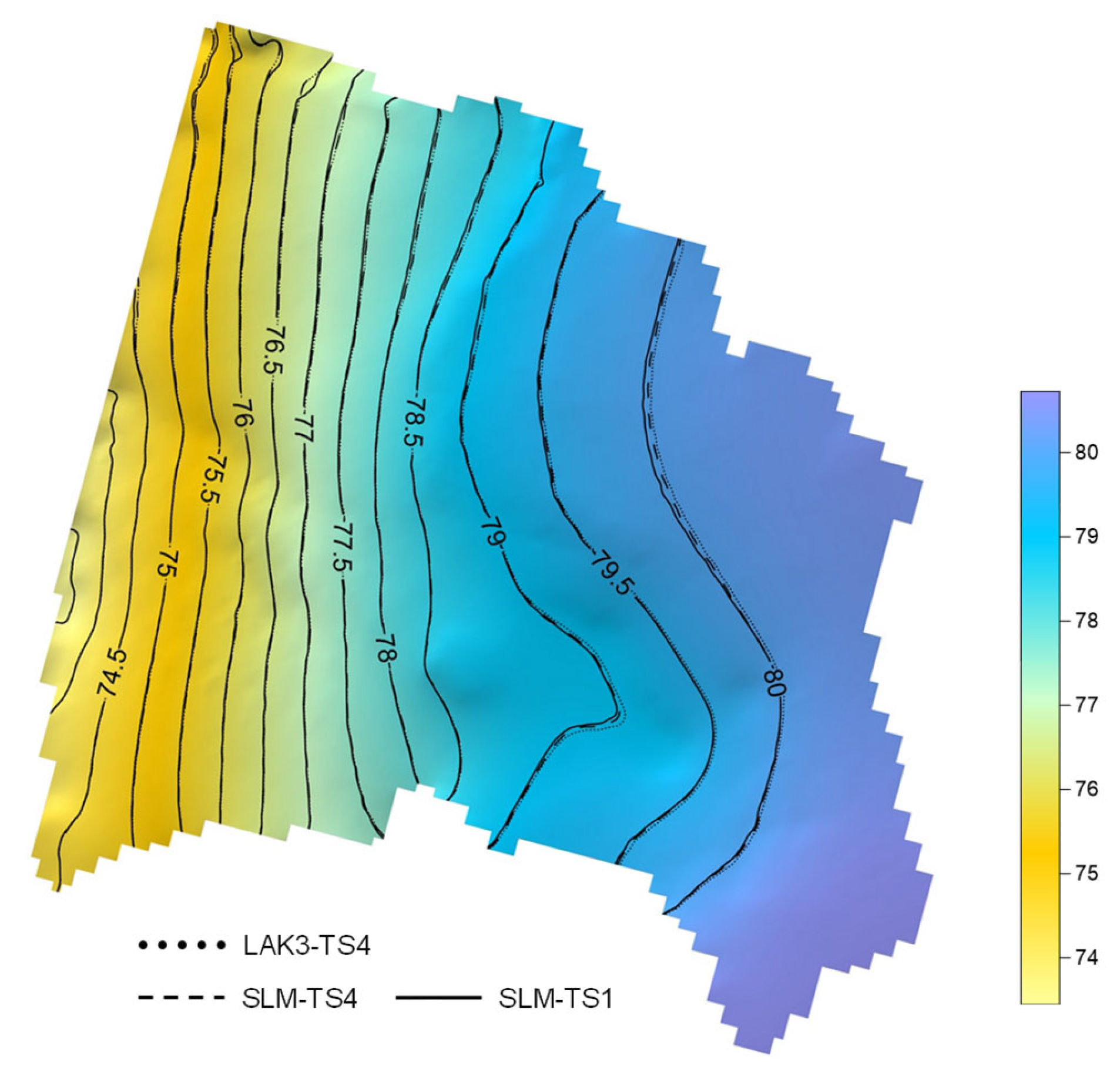
3.1. Simulated Groundwater Head

The simulation results of the groundwater head were verified by 32 hydraulic head observations, among which 6 were selected randomly for display. As shown in Figure 5, all model simulations fit well with the observations, with errors less than 1 m. The seasonal dynamics were reproduced successfully as well. The simulated groundwater head shows both overestimation (B1, B6, B8) and underestimation (B4, B7, B18) in comparison to the observed head, meaning that the models do not have a systematic bias. There is almost no difference between the LAK3-based model and SLM-based models.

The annual mean simulated groundwater head in 2008 is shown in Figure 6. It is seen that the three models under scrutiny exhibit almost identical spatial patterns of simulated heads. The average difference is 0.0002 m between LAK3-TS4 and SLM-TS4. When reducing the number of calculation layers for the lake from four to one in the SLM, it does not generate any noticeable impact on the simulated results, as the average groundwater head difference is only 0.003 m between SLM-TS4 and SLM-TS1.

Model performance statistics were calculated and summarized in

Table 1. Model performance and computational time.

		LAK3-TS4	SLM-TS4	SLM-TS1
Groundwater head	RMSE 1 (m)	0.289	0.291	0.292
	MAE 2 (m)	0.234	0.235	0.235
Lake level	RMSE (m)	0.049	0.048	0.049
	MAE (m)	0.039	0.036	0.037
Computational time	(s)	291	312	195

¹ RMSE indicates the Root Mean Square Error; ² MAE indicates the Mean Absolute Error.

. It shows that there is little difference in terms of simulated groundwater head between the LAK3-based model and SLM-based models. The one-layer model (SLM-TS1) has almost the same performance as the four-layer model (SLM-TS4), and the difference between them is negligible.

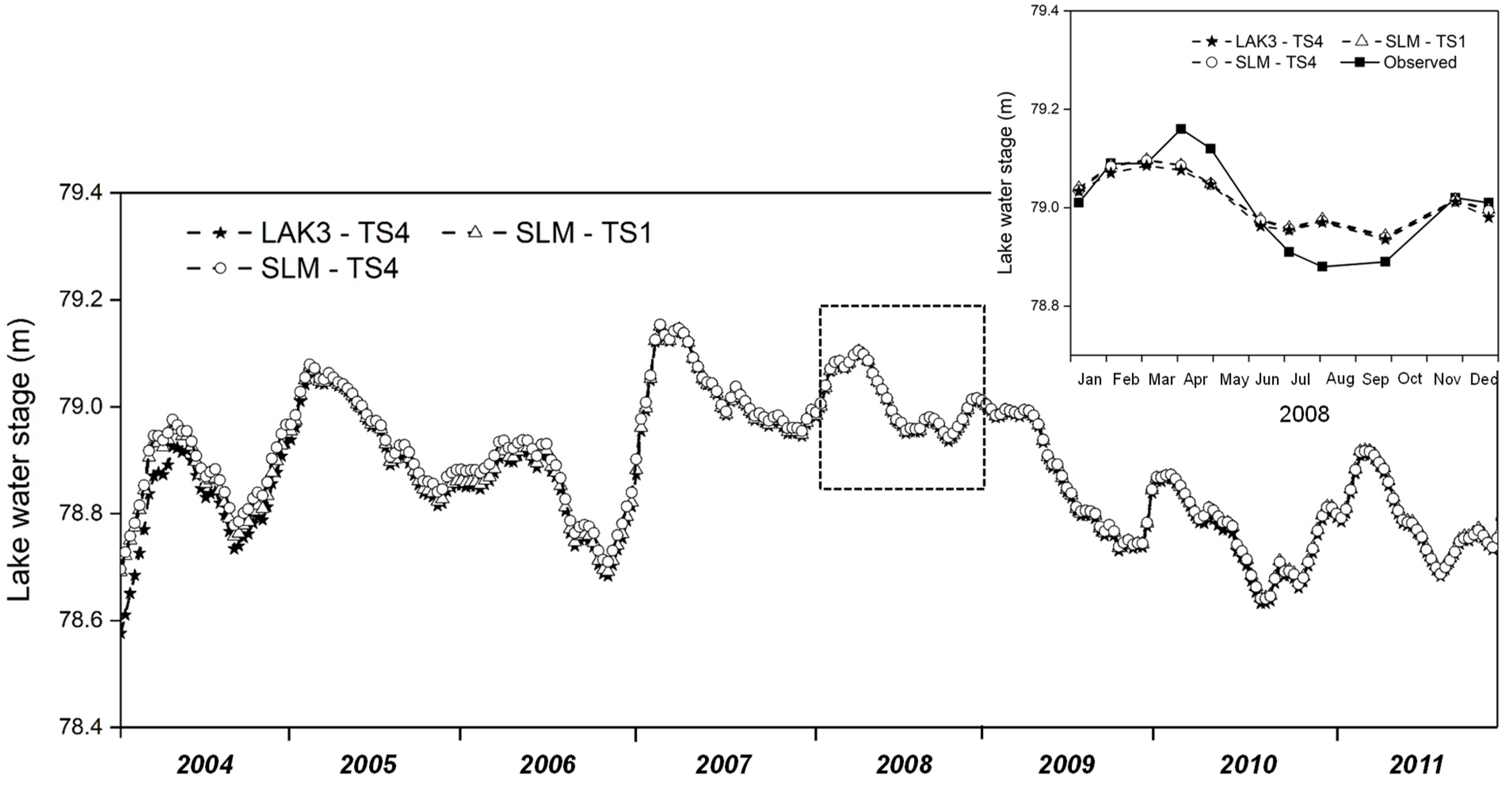
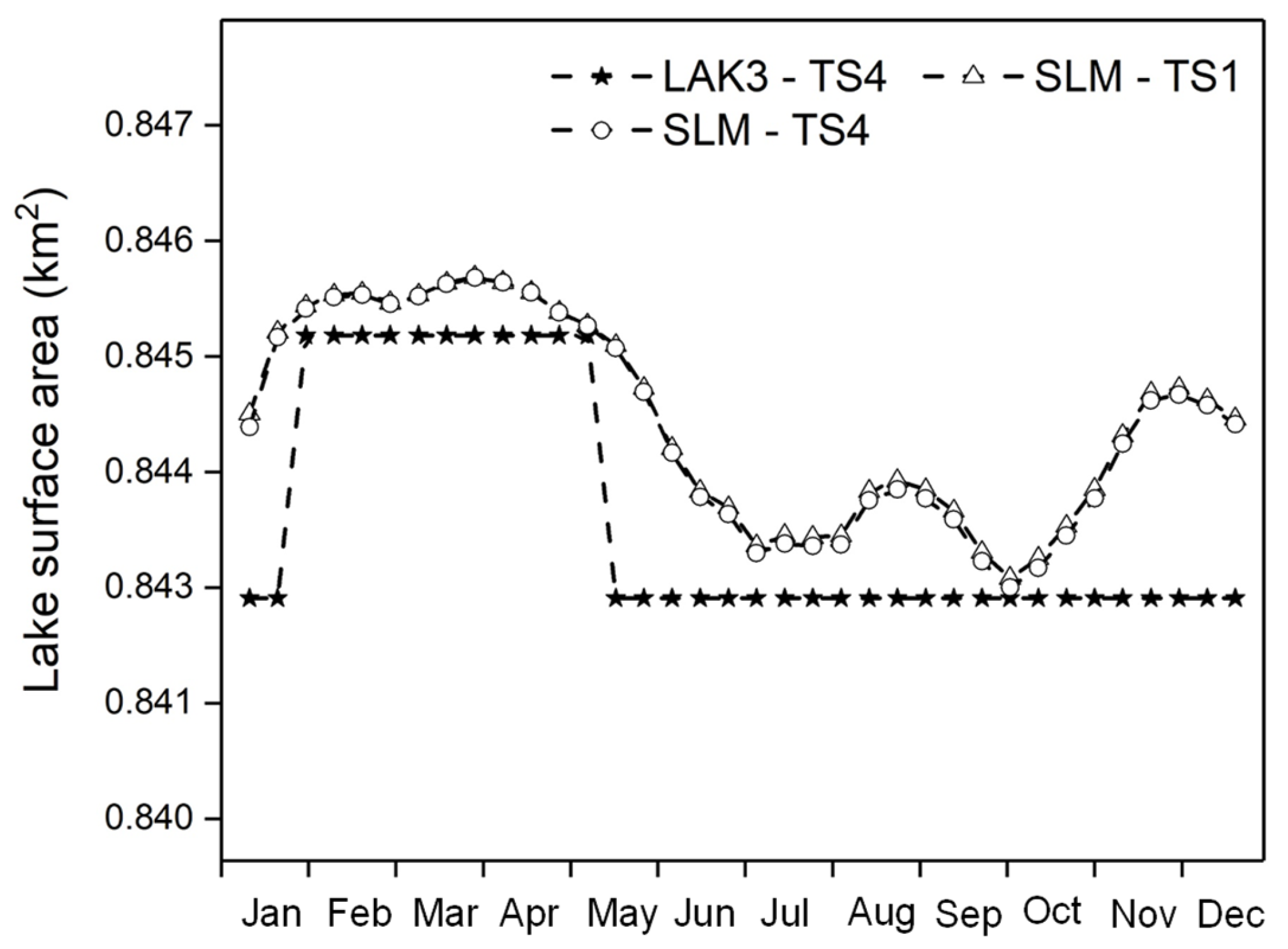
3.2. Simulated Lake Level and Surface Area

The observed and simulated lake water levels are shown in Figure 7. It is seen that all three models are able to reproduce the observed lake level in 2008 with acceptable accuracy. The SLM-based models (SLM-TS4 and SLM-TS1) have almost the same performance as the benchmark model (LAK3-TS4).

Such observation is also confirmed by Table 1, where the SLM-based model (SLM-TS4) has almost the same performance as the LAK3-based model (LAK3-TS4) in terms of simulated groundwater head and lake water level for both RMSE and MAE. When the number of layers representing the lake is reduced from four to one in the SLM, the model performance changes little.

Figure 8 shows the simulated lake surface area of the three models in 2008. It can be seen that the simulated lake surface area based on the SLM changes smoothly, which resembles the lake’s natural condition more, while the lake surface area simulated by the LAK3 method can only be at certain fixed values because the lakebed within the lakebed cells is sloped in the SLM. In contrast, the lakebed is flat in LAK3. For instance, from February to April, the lake surface area simulated by the LAK3 method is 0.845 km², while the SLM-based model increased the lake surface area from 0.845 km² to 0.846 km².

3.3. Simulated Water Balance

The water balances for the groundwater and the lake simulated by SLM and LAK3 are shown in

Table 2. Water balance for the groundwater in 2008.

		LAK3-TS4	SLM-TS4	SLM-TS1
In (mil. m3/year)	Recharge	11.713	11.711	11.711
	Stream Leakage	0.039	0.035	0.039
	Lake Seepage	1.677	1.650	1.655
	Head Dep Bounds	1.257	1.258	1.250
	Total	14.686	14.655	14.655
Out (mil. m3/year)	Lake Seepage	2.425	2.403	2.441
	Stream Leakage	0.031	0.031	0.032
	Head Dep Bounds	11.623	11.635	11.664
	Total	14.079	14.068	14.137
Storage Change (m3/year)		0.602	0.595	0.522
In-Out-ΔS		0.005	−0.009	−0.004
Water Balance Error (%)		0.035	0.062	0.029

and

Table 3. Water balance for Lake Hampen in 2008.

	Source/Sink Term	LAK3-TS4	SLM-TS4	SLM-TS1
In (mil. m3/year)	P	0.967	0.967	0.967
	Qsi	0.363	0.361	0.370
	Rnf	0	0	0
	$G_p^{in}+G_N^{in}$	2.425	2.403	2.441
	Total	3.755	3.731	3.778
Out (mil. m3/year)	E	0.523	0.523	0.523
	$G_p^{out}$	1.677	1.650	1.655
	W	0	0	0
	Qso	1.544	1.550	1.594
	Total	3.745	3.723	3.772
Storage Change (mil. m3/year)		0.01	0.008	0.006
In-Out-ΔS		0.01	0.008	0.006
Water Balance Error (%)		0	0	0

, respectively. It is seen in Table 2 that the main source of groundwater recharge is a really distributed recharge. The interaction between the lake and the groundwater is two-directional: there is both lake water leaking to groundwater and groundwater seeping into the lake. Overall, Lake Hampen was a charging lake in 2008, on average, with a positive net groundwater recharge. The groundwater flows out of the model domain through the west boundary due to the gradient in the landscape.

For Lake Hampen, it is mostly recharged by groundwater and precipitation, as shown in Table 3. The river inflow from upstream accounts for approximately 1/10 of the total lake recharge. It is shown in Table 2 and Table 3 that all three models can close the water balance rather successfully, with relatively small water balance errors. For groundwater, both the SLM-based models and LAK3 based-model have good performance (balance error of less than 0.1%). For the lake, the balance error for all three models is 0. Moreover, there is no significant difference in water balance performance when the number of lake layers is reduced from 4 to 1 in SLM, as shown in Table 2 and Table 3. The cumulative lake–groundwater interaction water volume simulated by the three models is shown in Figure 9. It can be seen that the simulation results of the three models are quite similar.

4. Discussion and Conclusions

4.1. SLM as a New Lake–Groundwater Simulation Tool

Benchmark problems in hydrogeology have traditionally been used to validate numerical codes and solvers by comparing their output in simplified cases with known analytical solutions. However, as model developments target increasingly complex problems, analytical solutions may no longer exist, implying that benchmarking needs to be carried out through model intercomparisons using real case studies, which is a greater challenge [31]. Comparative studies addressing real-world problems may reveal model strengths and/or weaknesses that otherwise would be hard to discover [32]. Due to the complex nature when lakes are coupled with groundwater, very few model codes exist for making simulations for such a purpose at a smaller scale, and, thus, only a few model intercomparison studies are found in the past literature regarding coupled lake–groundwater systems [33]. The SLM, as a newly developed lake–groundwater simulation tool, should be compared with known, well-performing model code to demonstrate its validity and, if possible, improvements. Therefore, the present study is a valuable addition to the intercomparison studies of the methods used in simulating lake–groundwater interactions.

Our comparison between the widely used MODFLOW Lake Package, LAK3 [28] and the newly developed SLM code [30] showed that they could, regardless of grid resolution, perform equally well in reproducing the observed lake water level and the groundwater level around the lake, as well as balancing the water budget. However, LAK3 requires a relatively high grid resolution (with multiple lake layers) to adequately represent the lake bathymetry, whereas the SLM is independent of the grid resolution of the groundwater model. This makes the latter more compatible with relatively coarse grids, even with, e.g., a single lake layer. Additionally, as far as lake surface area is concerned, the SLM has a better potential to emulate its natural fluctuation compared to LAK3, although more observed data are needed to verify such observation.

4.2. Savings in Computational Time

The computational time used by LAK3- and SLM-based models are summarized in Table 1, and it is shown that the one-layer SLM is able to shorten the computational times by more than 30% in transient flow simulation for Lake Hampen. In deterministic applications with a single lake in the model domain, one can expect a relatively short total computational time, e.g., five minutes or less, as seen in the Lake Hampen example, which could indicate that savings of model runtime may not be a priority for future model improvements.

However, in more complex model settings—for instance, when multiple lakes are of interest—flow models are interactively coupled with solute transport models, or, in cases where uncertainty needs to be addressed, computational time savings similar to the magnitude found in this study may be critical. More specifically, Monte Carlo-based scenario analyses involving a large number of simulations have been used to investigate groundwater–lake interactions [34] and nutrient transport in surface water–groundwater systems under the impacts of climate change [35,36]. In those cases, a time saving of 30% can be rather significant. Therefore, it is implied that the SLM may have the ability to reduce the need of using supercomputers when investigating the impacts of climate change on complex atmosphere–lake/surface water–groundwater systems [37] or solving inverse problems in simulations of contaminant source release history [38,39].

References

1. Dimova, N.T.; Burnett, W.C.; Chanton, J.P.; Corbett, J.E. Application of radon-222 to investigate groundwater discharge into small shallow lakes. J. Hydrol. 2013, 486, 112–122. [Google Scholar] [CrossRef]
2. Erik, J. Focused groundwater discharge of phosphorus to a eutrophic seepage lake (Lake Væng, Denmark): Implications for lake ecological state and restoration. Hydrogeol. J. 2013, 21, 1787–1802. [Google Scholar] [CrossRef]
3. Zhou, S.Q.; Kang, S.C.; Chen, F.; Joswiak, D.R. Water balance observations reveal significant subsurface water seepage from Lake Nam Co, south-central Tibetan Plateau. J. Hydrol. 2013, 491, 89–99. [Google Scholar] [CrossRef]
4. Pöschke, F.; Nützmann, G.; Engesgaard, P.; Lewandowski, J. How does the groundwater influence the water balance of a lowland lake? A field study from Lake Stechlin, north-eastern Germany. Limnologica 2018, 68, 17–25. [Google Scholar] [CrossRef]
5. Rossman, N.R.; Zlotnik, V.A.; Rowe, C.M. Simulating lake and wetland areal coverage under future groundwater recharge projections: The Nebraska Sand Hills system. J. Hydrol. 2019, 576, 185–196. [Google Scholar] [CrossRef]
6. Kidmose, J.; Engesgaard, P.; Ommen, D.A.O.; Nilsson, B.; Flindt, M.R.; Andersen, F.O. The Role of Groundwater for Lake-Water Quality and Quantification of N Seepage. Groundwater 2015, 53, 709–721. [Google Scholar] [CrossRef] [PubMed]
7. Lewandowski, J.; Meinikmann, K.; Nutzmann, G.; Rosenberry, D.O. Groundwater–the disregarded component in lake water and nutrient budgets. Part 2: Effects of groundwater on nutrients. Hydrol. Process. 2015, 29, 2922–2955. [Google Scholar] [CrossRef]
8. Chen, J.; Qian, H. Characterizing replenishment water, lake water and groundwater interactions by numerical modelling in arid regions: A case study of Shahu Lake. Hydrol. Sci. J. 2017, 62, 104–113. [Google Scholar] [CrossRef]
9. Urrutia, J.; Herrera, C.; Custodio, E.; Jodar, J.; Medina, A. Groundwater recharge and hydrodynamics of complex volcanic aquifers with a shallow saline lake: Laguna Tuyajto, Andean Cordillera of northern Chile. Sci. Total Environ. 2019, 697, 134116. [Google Scholar] [CrossRef]
10. Zhang, B.; Lu, C.Y.; Wang, J.H.; Sun, Q.Y.; He, X.; Cao, G.L.; Zhao, Y.; Yan, L.J.; Gong, B.Y. Using storage of coal-mining subsidence area for minimizing flood. J. Hydrol. 2019, 572, 571–581. [Google Scholar] [CrossRef]
11. Schneider, R.L.; Negley, T.L.; Wafer, C. Factors influencing groundwater seepage in a large, mesotrophic lake in New York. J. Hydrol. 2005, 310, 1–16. [Google Scholar] [CrossRef]
12. Mccobb Timothy, D.; Briggs Martin, A.; Leblanc Denis, R.; Day-Lewis Frederick, D.; Johnson Carole, D. Evaluating long-term patterns of decreasing groundwater discharge through a lake-bottom permeable reactive barrier. J. Environ. Manag. 2018, 220, 233. [Google Scholar] [CrossRef]
13. Tirado-Conde, J.; Engesgaard, P.; Karan, S.; Muller, S.; Duque, C. Evaluation of Temperature Profiling and Seepage Meter Methods for Quantifying Submarine Groundwater Discharge to Coastal Lagoons: Impacts of Saltwater Intrusion and the Associated Thermal Regime. Water 2019, 11, 1648. [Google Scholar] [CrossRef]
14. Campodonico, V.A.; Dapena, C.; Pasquini, A.I.; Lecomte, K.L.; Piovano, E.L. Hydrogeochemistry of a small saline lake: Assessing the groundwater inflow using environmental isotopic tracers (Laguna del Plata, Mar Chiquita system, Argentina). J. S. Am. Earth Sci. 2019, 95, 102305. [Google Scholar] [CrossRef]
15. Smith, R.L.; Repert, D.A.; Stoliker, D.L.; Kent, D.B.; Song, B.; LeBlanc, D.R.; McCobb, T.D.; Bohlke, J.K.; Hyun, S.P.; Moon, H.S. Seasonal and spatial variation in the location and reactivity of a nitrate-contaminated groundwater discharge zone in a lakebed. J. Geophys. Res.-Biogeosci. 2019, 124, 2186–2207. [Google Scholar] [CrossRef]
16. Kidmose, J.; Engesgaard, P.; Nilsson, B.; Laier, T.; Looms, M.C. Spatial Distribution of Seepage at a Flow-Through Lake: Lake Hampen, Western Denmark. Vadose Zone J. 2011, 10, 110–124. [Google Scholar] [CrossRef]
17. Nisbeth, C.S.; Kidmose, J.; Weckstrom, K. Dissolved inorganic geogenic phosphorus load to a groundwater-fed lake: Implications of terrestrial phosphorus cycling by groundwater. Water 2019, 11, 2213. [Google Scholar] [CrossRef]
18. Tecklenburg, C.; Blume, T. Identifying, characterizing and predicting spatial patterns of lacustrine groundwater discharge. Hydrol. Earth Syst. Sci. 2017, 21, 5043–5063. [Google Scholar] [CrossRef]
19. Abbo, H.; Shavit, U.; Markel, D.; Rimmer, A. A numerical study on the influence of fractured regions on lake/groundwater interaction; the Lake Kinneret (Sea of Galilee) case. J. Hydrol. 2003, 238, 225–243. [Google Scholar] [CrossRef]
20. Ala-Aho, P.; Rossi, P.M.; Isokangas, E.; Kløve, B. Fully integrated surface-subsurface flow modelling of groundwater-lake interaction in an esker aquifer: Model verification with stable isotopes and airborne thermal imaging. J. Hydrol. 2015, 522, 391–406. [Google Scholar] [CrossRef]
21. Yihdego, Y.; Webb, J.A.; Leahy, P. Modelling of lake level under climate change conditions: Lake Purrumbete in southeastern Australia. Environ. Earth Sci. 2015, 73, 3855–3872. [Google Scholar] [CrossRef]
22. Smerdon, B.D.; Mendoza, C.A.; Devito, K.J. Simulations of fully coupled lake-groundwater exchange in a subhumid climate with an integrated hydrologic model. Water Resour. Res. 2007, 43, WO1416. [Google Scholar] [CrossRef]
23. Sacks, L.A.; Herman, J.S.; Konikow, L.F.; Vela, A.L. Seasonal dynamics of groundwater-lake interactions at Doñana National Park, Spain. J. Hydrol. 1992, 136, 123–154. [Google Scholar] [CrossRef]
24. Dogan, A.; Karaguzel, R.; Soyaslan, I.I. Modelling of lake—Groundwater interaction in Turkey. Water Manag. 2008, 161, 277–287. [Google Scholar] [CrossRef]
25. Hunt, R. Ground water-lake interaction modeling using the LAK3 package for MODFLOW 2000. Groundwater 2005, 41, 114. [Google Scholar] [CrossRef]
26. Yihdego, Y.; Reta, G.; Becht, R. Human impact assessment through a transient numerical modeling on the UNESCO World Heritage Site, Lake Naivasha, Kenya. Environ. Earth Sci. 2017, 76, 9. [Google Scholar] [CrossRef]
27. Cheng, X.X.; Anderson, M.P. Numerical simulation of ground-water interaction with lakes allowing for fluctuating lake levels. Groundwater 1993, 31, 929–933. [Google Scholar] [CrossRef]
28. Merritt, M.L.; Konikow, L.F. Documentation of a Computer Program to Simulate Lake-Aquifer Interaction Using the MODFLOW Ground-Water Flow Model and the MOC3D Solute-Transport Model; U.S. Geological Survey: Reston, VA, USA, 2000. [CrossRef]
29. Hunt, R.J.; Haitjema, H.M.; Krohelski, J.T.; Feinstein, D.T. Simulating ground water-lake interactions:Approaches and insights. Groundwater 2003, 41, 227–237. [Google Scholar] [CrossRef]
30. Lu, C.; Zhang, B.; He, X.; Cao, G.; Sun, Q.; Yan, L.; Qin, T.; Li, T.; Li, Z. Simulation of lake-groundwater interaction under steady-state flow. Groundwater 2020, 59, 90–99. [Google Scholar] [CrossRef]
31. Maxwell, R.M.; Putti, M.; Meyerhoff, S.; Delfs, J.O. Surface-subsurface model intercomparison: A first set of benchmark results to diagnose integrated hydrology and feedbacks. Water Resour. Res. 2014, 50, 1531–1549. [Google Scholar] [CrossRef]
32. Finsterle, S.; Lanyon, B.; Åkesson, M. Conceptual uncertainties in modelling the interaction between engineered and natural barriers of nuclear waste repositories in crystalline rocks. Geol. Soc. Lond. Spec. Publ. 2019, 482, 261–283. [Google Scholar] [CrossRef]
33. Van Loon, A.F.; Van Huijgevoort, M.H.J.; Van Lanen, H.A.J. Evaluation of drought propagation in an ensemble mean of large-scale hydrological models. Hydrol. Earth Syst. Sci. 2012, 16, 4057–4078. [Google Scholar] [CrossRef]
34. Elsawwaf, M.; Feyen, J.; Batelaan, O.; Bakr, M. Groundwater–surface water interaction in lake Nasser, Southern Egypt. Hydrol Process. 2014, 28, 414–430. [Google Scholar] [CrossRef]
35. Jarsjo, J.; Tornqvist, R.; Su, Y. Climate-driven change of nitrogen retention–attenuation near irrigated fields: Multi-model projections for Central Asia. Environ. Earth Sci. 2017, 76, 117. [Google Scholar] [CrossRef]
36. Jarsjo, J.; Andersson-Skold, Y.; Froberg, M.; Pietron, J.; Borgstrom, R.; Lov, A.; Kleja, D.B. Projecting impacts of climate change on metal mobilization at contaminated sites: Controls by the groundwater level. Sci. Total Environ. 2020, 712, 135560. [Google Scholar] [CrossRef]
37. Beigi, E.; Tsai, F.T.C. Comparative study of climate-change scenarios on groundwater recharge, southwestern Mississippi and southeastern Louisiana, USA. Hydrogeol. J. 2015, 23, 789–806. [Google Scholar] [CrossRef]
38. Sayeed, M.; Mahinthakumar, G.K. Efficient parallel implementation of hybrid optimization approaches for solving groundwater inverse problems. J. Comput. Civil Eng. 2005, 19, 329–340. [Google Scholar] [CrossRef]
39. Deng, X.M.; Cai, X.C.; Zou, J. Two-level space–time domain decomposition methods for three-dimensional unsteady inverse source problems. J. Sci. Comput. 2016, 67, 86–882. [Google Scholar] [CrossRef]
Figure 1. Location of Lake Hampen and the model domain.
Water 14 03054 g001
Figure 2. Conceptual models of the lake packages to be coupled with MODFLOW: (a) Plain view and (b) side view of a lake. Lakebed conceptualization using the (c) LAK3 method and (d) SLM method. For the SLM,   P is precipitation, E is evaporation,   W is water withdrawal, Q s i is inflow from upstream rivers to the lake, Q s o is outflow from the lake to downstream rivers,   G p i n is inflow from groundwater to the lake in the submerged area, G p o u t is outflow from the lake to groundwater in the submerged area,   R n f is the surface runoff generated in the unsubmerged area, G N i n is groundwater seepage to the unsubmerged area. For LAK3, Q r n f is the surface runoff to the lake, and s p is the net seepage between the lake and the aquifer.
Water 14 03054 g002
Figure 3. Configuration of the groundwater flow model and lake modules. (a) Plain view of the model domain: horizontal discretization, boundary conditions and observation wells. (b) Side view of the model domain at A–A′ for LAK3: vertical discretization, hydrogeological units and lake grid cells. (c,d) Side view of the model domain at A–A′ for the SLM: vertical discretization, hydrogeological units and grid cells with four layers (SLM-TS4) and one layer (SLM-TS1).
Water 14 03054 g003
Figure 4. Groundwater recharge zones. Zone 0: Lake Hampen, Zone 1: Coniferous forest with an unsaturated zone thickness less than 5 m, Zone 2: Grass with an unsaturated zone thickness less than 5 m, Zone 3: Forest with an unsaturated zone thickness larger than 5 m, Zone 4: Grass with an unsaturated zone thickness larger than 5 m.
Water 14 03054 g004
Figure 5. Comparison of the observed and simulated groundwater head at six different groundwater observation wells in 2008 (well locations are shown in Figure 3).
Water 14 03054 g005
Figure 6. Spatial distribution and contour of simulated groundwater head in 2008.
Water 14 03054 g006
Figure 7. Comparison of observed and simulated lake level.
Water 14 03054 g007
Figure 8. Simulated lake surface area in 2008.
Water 14 03054 g008
Figure 9. Cumulative Lake–Groundwater interaction water volume since the initial time.
Water 14 03054 g009