Abstract
Accurate estimation of precipitation patterns is essential for the modeling of hydrological systems and for the planning and management of water resources. However, rainfall time series, as obtained from traditional rain gauges, are frequently corrupted by missing values that might hinder frequency analysis, hydrological and environmental modeling, and meteorological drought monitoring. In this paper, we evaluated three techniques for filling missing values at daily and monthly time scales, namely, simple linear regression, multiple linear regression, and the direct imputation of satellite retrievals from the Global Precipitation Measurement (GPM) mission, in rainfall gauging stations located in the Brazilian midwestern region. Our results indicated that, despite the relatively low predictive skills of the models at the daily scale, the satellite retrievals provided moderately more accurate estimates, with better representations of the temporal dynamics of the dry and wet states and of the largest observed rainfall events in most testing sites in comparison to the statistical models. At the monthly scale, the performance of the three methods was similar, but the regression-based models were unable to reproduce the seasonal characteristics of the precipitation records, which, at least to some extent, were circumvented by the satellite products. As such, the satellite retrievals might comprise a useful alternative for dealing with missing values in rainfall time series, especially in those regions with complex spatial precipitation patterns.
1. Introduction
Precipitation is one of the main elements of the global water and energy cycles, which regulates climate systems [1], and controls the availability of surface water and the recharge conditions in both time and space. Such a variable is a key component of the water budget in a given region and exerts a direct influence on its ecological and economic dynamics [2]. Therefore, accurate estimation and monitoring of precipitation patterns are essential for the modeling of hydrological systems, as well as for the planning and management of water resources in various sectors of society [3], such as human supply, hydropower generation, agriculture, land-use planning, and drought management and mitigation [4].
Rainfall data is traditionally obtained from rainfall gauges (i.e., pointwise). These instruments are considered the reference data source for precipitation observations as they provide direct measurements of precipitation at a given site [5]. However, even when information with fine-time resolution is available, rain gauges may not capture the spatial variability of precipitation fields in large areas or in regions with a complex topography [5,6,7]. Moreover, equipment malfunctions or human errors frequently affect recording procedures, which may entail unreliable estimates of variables indirectly obtained from hydrological and environmental models [8]. Finally, limitations still persist with respect to the density of the gauging network and the periods of record of the available gauges, which may hinder the proper characterization of the rainfall stochastic process at the locations of interest [9,10].
Another issue frequently verified in ground-based rainfall time series is the existence of missing values, i.e., points in time in which no measurement is performed. Missing data in rainfall time series may also strongly affect statistical analysis, both with respect to the probabilities of wet and dry states of the process and to the description of its extremes [11]. In effect, the existence of missing values during wet spells (at shorter time scales) might conceal the largest rainfall amounts during a given time window (e.g., a water year). This may entail the loss of useful information for describing the decay of the upper tails of the parent or the block-maxima distributions of precipitation volumes for a given duration and increase the effects of sampling errors in parameter and quantile estimates. On the other hand, long periods of missing data during dry seasons (or larger time scales) may affect meteorological drought assessment, regarding the mean and maximum duration and severity of extreme events [12]. In a more general context, missing values may compromise the reliability of stochastic simulations of the rainfall process (e.g., [11,13]), as well as rainfall–runoff modeling expedients. Thus, pre-processing of the raw data set for filling missing values in the rainfall time series is a frequently required in hydrological studies [14].
Methods for filling missing rainfall values are designed for constructing complete data sets by imputing model-based rainfall estimates to the corrupted time series. The most common techniques for this purpose are the regional weighting method, linear regression models, and regional vectors [15]. Additionally, the gauge mean estimator [16], the inverse distance weighting method [17], and ordinary Kriging [18,19,20] have been increasingly used because of their simplicity and ease of application. Although very distinct in their mathematical formalism, these methods are based on a similar rationale: information recorded at nearby sites is utilized for estimating the missing values at the target location by means of an “averaging” process. However, according to [21], due to the marked spatial variability and intermittence of the rainfall process at fine time scales, such approaches are more recommended for filling monthly and annual rainfall amounts; the aggregation process smooths out the higher-resolution time series, which attenuates the effects of small timescale extremes and dry spells and might strongly reduce estimation errors [11]. On the other hand, daily and sub-daily precipitation information are basic inputs for hydrological models and rainfall frequency analysis, but, in general, models for filling missing values at such small timescales are scarce and affected by low predictive abilities due to the high levels of variability of the process [22,23].
As a means of tackling this problem, it is usual to discard those years (or other time windows) in which missing values occur. This, however, might result in very short samples or hinder the proper description of the upper tail of the random variable distribution [24]. Alternatively, one might resort to regression-based techniques for estimating the missing values when the modeling errors are acceptable, but this is an unusual situation for daily data. Previous research has discussed the use of multiple linear regression [25], simple substitution [14], the Theil method [26], and machine-learning algorithms [27,28] for this purpose, but the effectiveness of these methods is still inherently dependent on the ability of the gauging network to reproduce the observed rainfall fields, particularly those with complex spatial patterns, and the more extreme events. As a result, the filling of missing rainfall data at the daily (or shorter timescale) remains an open research field [24,29].
In recent years, the use of precipitation estimates retrieved from remote-sensing data sources, such as satellites, has gained popularity among researchers and practitioners around the world, especially in regions with poor density gauging [30]. In fact, satellites provide products with high sampling frequencies, improved spatial resolution at large catchments or regions, not corrupted by missing data, and with low costs for the end-users [31]. On the other hand, due to the limitations of the retrieval algorithms, satellite estimates are frequently biased, even after time-averaging [32], which might hinder their utilization without pre-processing or bias correction [33]. Yet, the levels of bias may considerably vary for distinct intervals of rainfall amounts (e.g., [34]) and, at least for some ranges, the satellite retrievals may reasonably agree with ground-based information. This fact has prompted the research question as to whether utilizing satellite rainfall estimates for filling missing data in rainfall gauging stations enclosed by a satellite pixel comprises a more effective and accurate alternative than using data from nearby sites.
Recent papers have addressed this rationale for filling missing rainfall values at large time scales, such as monthly or the seasonal ones [35,36,37]. However, to the best of our knowledge, the use of satellite retrieval for filling daily rainfall data has not been fully explored in the literature. To address this potential research gap, the main objective of this study is assessing the feasibility of direct imputation of remote sensing data provided by Global Precipitation Measurement (GPM) satellites, via the Integrated Multi-satellite Retrievals for GPM (IMERG) algorithm, for filling the missing data in rain gauges. For this, we evaluated whether this framework yielded better results, at daily and monthly time scales, as compared to traditional regression-based methods, namely, multiple linear regression (MLR) with fixed “donor” sites, and simple linear regression (SLR), which utilizes a single “donor” site that may otherwise vary due to information availability in nearby stations, in a collection of rain gauges in the midwestern Brazilian region. The remainder of the paper is organized as follows. Section 2 presents material and methods, with a brief description of the study area and the data, as well as the methods utilized for filling missing values in precipitation time series and for performance assessment. Section 3 comprises the main results and discussion with respect to previous research. Finally, in Section 4, conclusions and research developments are addressed.
2. Material and Methods
2.1. Study Area and Rainfall Data
The study area encompassed the central and southern portions of the state of Goiás, in the Brazilian midwestern region (Figure 1). The study region is characterized by tropical savanna climate, with a dry season spanning from April to September and a wet season between October and March. Temperatures range from 17 °C to 31 °C, whilst the mean annual rainfall amounts vary from 1100 to 1800 mm. As for topography, important altimetric variations are observed, particularly in the northeastern portion of the study area, and the relief can be characterized from smooth to wavy [38].
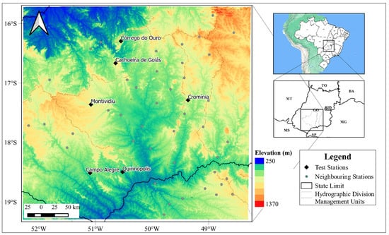
Figure 1.
Study area and location rainfall gauging stations utilized in this study.
Daily rainfall data were retrieved from 50 gauging stations operated by the Brazilian Agency of Water and Sanitation (ANA) (Table 1). These stations, which comprised periods of record of at least 30 years, are located in the southeastern region of the state of Goiás (Figure 1). A simplified data quality check was performed for excluding those years with more than 20% of missing data (which indirectly defined the periods of record utilized in the calibration of the models) and those with mean annual rainfall lower than 1000 mm and larger than 2500 mm, which were deemed unreasonable in the study area on the basis of previous research [38].

Table 1.
Rainfall gauging stations utilized in the study.
For assessing the predictive abilities of the regression-based models for filling daily missing data, 6 gauging stations were randomly selected from the ensemble as testing sites (Figure 1). Next, a complete water year of data, spanning from 1 September 2016 to 31 August 2017, was discarded, and the corresponding estimates were obtained with the MLR and the SLR models, as explained in Section 2.3, and imputed in the original time series. We note that this water year was selected for analyses because, along the interval in which the ground-based information overlapped the IMERG-GPM product (i.e., from 2014 onwards), this was the only period in which no missing data were verified at the “donor” sites utilized for both simple and multiple linear regression. A similar reasoning was utilized for the monthly time scale. We note, however, that the neighbor gauging stations utilized as “donor” sites may be different for these distinct time scales.
2.2. Data from the Global Precipitation Measurement Satellites
By means of the IMERG algorithm, the GPM mission combines data from all passive microwave instruments in the GPM satellite constellation to provide precipitation estimates, which are then merged and interpolated with estimates from calibrated infrared observations and other potential sensors at a spatial resolution of 0.1° × 0.1° and temporal resolution of 30 min across the globe [39].
In this study, the satellite retrievals were obtained from the NASA EarthData website in HDF5 format, and then converted to TIFF format using ArcGis 10.1. Then, the precipitation data—estimated in mm/h every 30 min, for each pixel enclosing the rainfall-gauging stations under study—were extracted. Finally, the data were aggregated to the daily time scale, using the interval from 7:00 am of one day until 6:59 am of the next day as a reference for matching the measurement interval of the gauges.
2.3. Filling of Missing Data
Traditional techniques for filling missing values in the precipitation time series, whether on annual, monthly, or daily time scales, are mainly based on spatial interpolation (i.e., the values to be imputed at the target site are calculated using synchronous observations from one or more neighbor stations) [24]. The following subsections describe two statistical methods, namely, multiple linear regression with fixed “donor” sites (MLR) and simple linear regression with variable “donor” sites (SLR). Then, the approach for imputing satellite retrievals is discussed.
2.3.1. Multiple Linear Regression (MLR) with Fixed “Donor” Sites
The MLR method for filling missing values, as proposed by Tabony (1983) [40], utilizes data from nearby sites as explanatory variables in the regression equation. Formally, for applying the MLR model, one must use at least two independent variables (“donor” sites). The rainfall amount to be estimated at the target site (dependent variable) is then related to N independent variables, as expressed in Equation (1):
in which is the estimated value for the dependent variable; is the intercept; are regression coefficients; and are the rainfall amounts at the “donor” sites (recorded simultaneously to the dependent variables in the calibration dataset). Parameters were estimated by means of the least squares method.
For avoiding overfitting, only those “donor” stations with significant linear relationship with the target sites (according to partial F tests at the 5% significance level) are included in the regression equations. Hence, for each target site, model identification proceeds as follows
- At least a pair of neighbor stations (with the highest levels of linear correlation), which do not have missing values along the period to be filled at the target site, is selected for composing the regression model. We restrict our attention to those “donor” stations located within a radius of 100 km of the target site for, at least to some extent, preserving similar climate conditions. More distant gauging stations (at most 150 km) are considered only in those cases in which the aforementioned criteria are not met;
- Other gauging stations are sequentially included in the model according to the linear correlation level with the target site. Then, partial F tests, at the 5% significance level, are performed for assessing whether the inclusion of a given station improves the predictive abilities of the regression model [41].
- The procedure is repeated until the inclusion of any of the remaining gauging stations does not significantly improve the models.
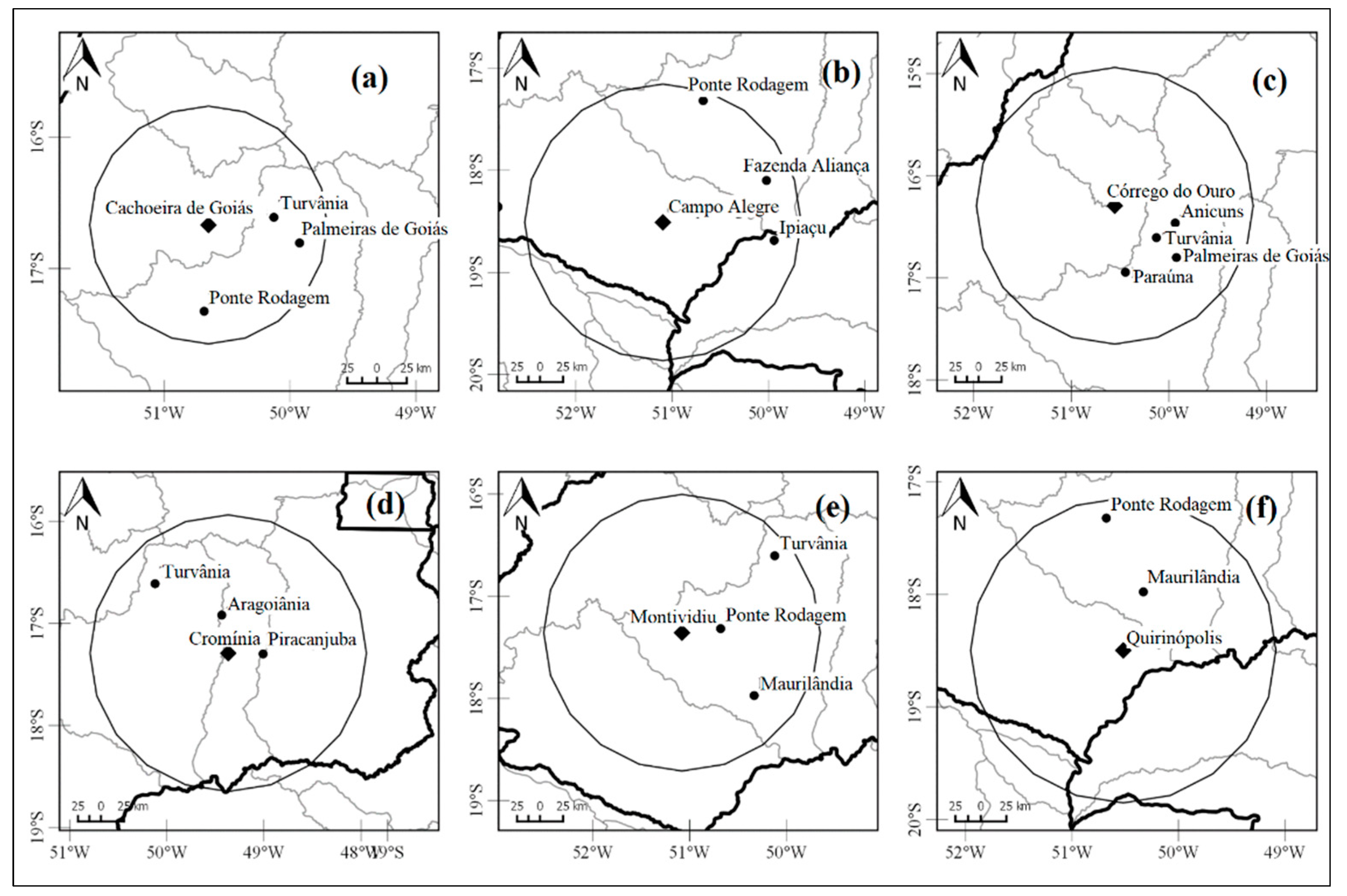
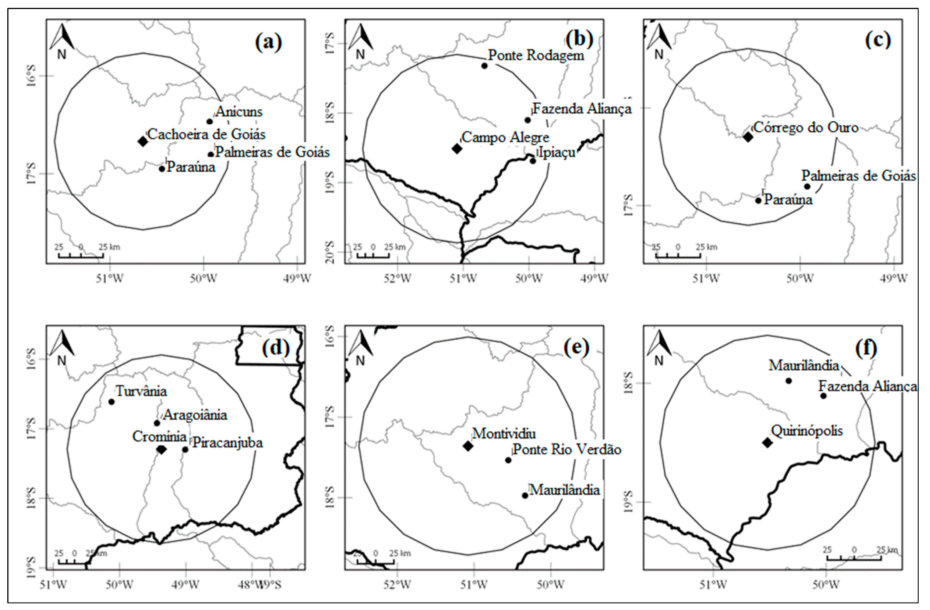
We note that the multiple regression equation allows for the inclusion of an intercept (or bias term), which enables the translation of the regression hyperplane towards the equality counterpart. In other words, systematic trends of under/overestimation of the MLR equation may be, at least to some extent, corrected by the model. However, the bias term, yet small, may prevent the simulation of null rainfall amounts in the target sites. Moreover, since no missing data are allowed in the “donor” sites during the period in which rainfall amounts are to be estimated at the target station, the most linearly correlated sites may not be included in the MRL equation. All steps for deriving the MLR equations are performed in RStudio interface of the R software. The “donor” stations for the previously selected target sites are depicted in Figure 2, for the daily time scale, and Figure 3, for the monthly counterpart.
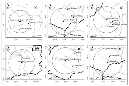
Figure 2.
Locations of the target sites and their respective” donor” stations for filling daily rainfall values with the multiple linear regression models: (a) Cachoeira de Goiás 100, (b) Campo Alegre 150, (c) Córrego do Ouro, (d) Cromínia, (e) Montividiu, and (f) Quirinópolis.
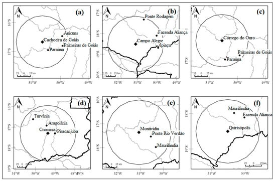
Figure 3.
Locations of the target sites and their respective “donor” stations for filling monthly rainfall values with the multiple linear regression model. Test stations: (a) Cachoeira de Goiás (b) Campo Alegre (c) Córrego do Ouro (d) Cromínia (e) Montividiu, and (f) Quirinópolis.
2.3.2. Simple Linear Regression (SLR) with Variable “Donor” Sites
Here, we resort to the framework described in the “hyfo” R package for estimating missing rainfall amounts from a single (yet variable) “donor” site. In short, the procedure for filling missing data, at daily, monthly, and annual time scales, is as follows. First, the Pearson correlation coefficient between the rainfall time series at the target site and each of the “donor” stations is computed (excluding the sample points with missing data). Next, the “donor” stations are ranked on the basis of the levels of linear correlation. Then, simple regression models, without the bias terms for allowing the simulation of null values, are identified for each pair of target and “donor” stations, according to Equation (2)
in which is the regression coefficient and x is the rainfall amount at a given “donor” site. Finally, the missing values at the target site are estimated from the linear model derived for the gauging station with the highest value of the Pearson correlation coefficient and available data. This is simpler yet more flexible than the MRL approach; since the requirements of data availability in all gauges during the period of missing data at the target site are relaxed whenever the best “donor” station has a missing value, the next best gauging station may provide the predictor for the linear model. However, as per the original implementation of the R package, intercepts, which may remove systematic bias from the model estimates (i.e., offsets from the 1:1 line), are not included in the regression equation. Hence, model performance is inherently dependent on the level of linear correlation between the target and the selected “donor” station. Yet, the SLR models might provide a useful benchmark for comparing the performances of the MLR models and the imputation of satellite retrievals.
2.3.3. Imputation of Satellite Retrievals
In this approach, we utilize the satellite retrievals from the pixel that encloses each of the target sites, as obtained from the IMERG-GPM product, for direct imputation, at both daily and monthly time scales. We note that such an expedient, albeit simple, has been disputed in the literature since it requires the downscaling of spatial-averaged precipitation in relatively large pixels to a point (i.e., the rainfall gauge) [42]. Moreover, satellite estimates are acknowledged biased, and the level of bias might be affected by long-term climate characteristics, seasonality, and topography [43,44]. However, since bias correction on the daily time scale is usually ineffective along the entire range of precipitation amounts [33], and defining appropriate intervals for removing bias from rainfall estimates is not straightforward, we rely on the raw satellite data for filling missing values; at least for some ranges, the satellite estimate may closely resemble ground-based information. A potential advantage of this rationale is that it might make filling missing data easier for practitioners.
2.4. Comparison of Methods
For assessing the performances of the different methods utilized for filling missing values in daily and monthly precipitation time series, the following metrics are used:
- Mean Absolute Error (MAE)
The MAE represents the average amplitude of the absolute error. It is represented by Equation (3):
- Root Mean Square Error (RMSE)
The RMSE measures the amplitude of the average squared error; hence, it more strongly penalizes larger errors than MAE, which is useful for assessing whether the lack of fit is restricted to highest order statistics or the entire range of rainfall amounts. It is represented by Equation (4):
- Percent Bias (PBias)
The percent bias is used to assess systematic errors. It can quantify tendencies of underestimation and overestimation of the estimated values with respect to the observations, as represented by Equation (5):
- Correlation Coefficient (CC)
The correlation coefficient reflects the degree of linear correlation between estimated and observed values, as represented by Equation (6):
In Equations (3)–(6), is the number of days, months, or years of imputed values, are the observed values, and are the values estimated by the method for filling missing values.
3. Results and Discussion
3.1. Daily Estimates
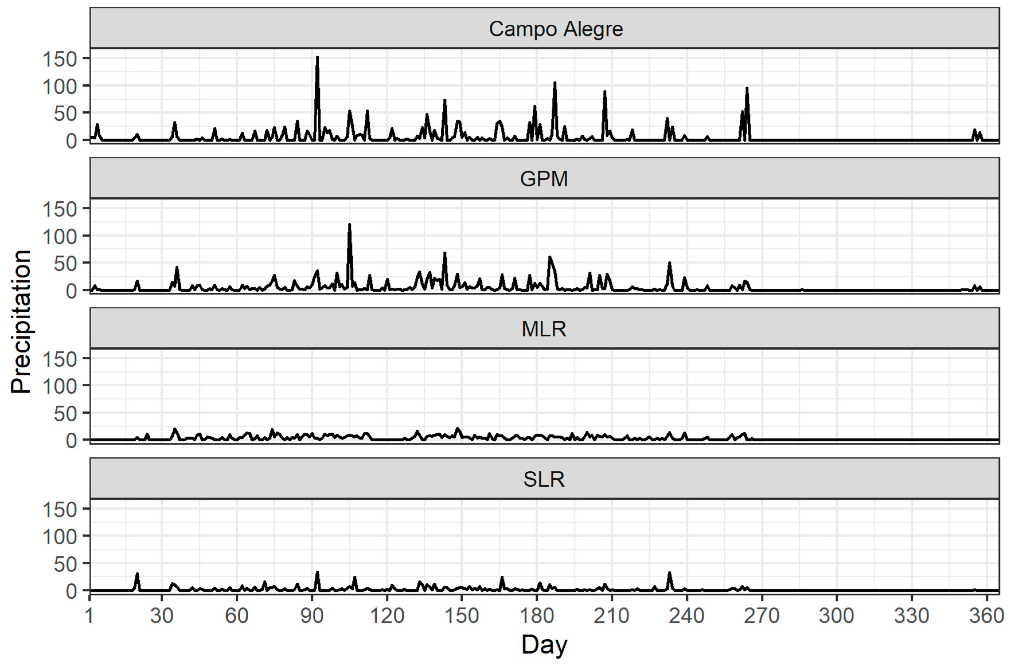
Table 2 presents performance assessment of the three methods for filling missing values, in the six testing sites, at the daily time scale (the method with better values for each metric is highlighted in bold). One may notice that, albeit all methods presented relatively low prediction skills, the direct imputation of the IMERG-GPM retrievals led to moderately more accurate results in most cases. In fact, the raw satellite data entailed higher values for the correlation coefficient (0.53, on average) and lower values of RMSE (9.7 mm, on average) in at least four target sites. Exceptions can be made in the Cachoeira de Goiás and the Campo Alegre gauging stations, in which direct imputation performed worse than the regression-based methods in terms of RMSE, and similarly to SLR with respect to the correlation coefficient. As a matter of fact, the GPM product considerably overestimated the observed annual rainfall (~317mm) at the former site, which presented the second-lowest observed annual rainfall, but the highest differences with respect to the satellite retrievals, both with respect to the cumulative process and to the observed daily extremes,. On the other hand, the satellite retrievals underestimated the rainfall amounts at the latter site (~217 mm), in which the highest annual precipitation and some of the largest rainfall amounts at the daily scale (>100 mm) were observed. We note that both sites are located in regions with weak topographic gradients, which should, at least to some extent, exclude the influence of terrain complexity in the relatively poor performance of the satellite product [33]. However, some influence of long-term climate conditions and of the variability of rainfall extremes [34,45] is apparently perceived in these sites.

Table 2.
Performance indexes of the three methods for filling daily missing data at the target sites.
It is also worth noting that the GPM product performed similarly, in terms of MAE (4.1 mm, on average), to the MLR models (4.0 mm, on average). However, since the former presented lower values of RMSE, one may infer that larger rainfall amounts are more accurately reproduced by the satellite retrievals. As for PBias (4%, on average), two gauging stations, namely, Cachoeira de Goiás, and Montividiu, presented strong tendencies of overestimation, whereas the remaining gauges were less biased, with prevailing behavior towards negative values. As previously stated, the satellite product could not reproduce the observed rainfall in the Cachoeira de Goiás gauging station in overall terms, which may justify the large bias at this site. However, at the Montividiu gauging station, the other metrics indicated the best performance of the satellite retrievals among the evaluated methods. We note that the GPM product also overestimated the annual rainfall amounts in Montividiu but, in this case, the differences in daily extremes were not too marked. Hence, we believe that the positive bias may have stemmed from a large number of false alarms by the satellite product, i.e., relatively small rainfall amounts captured by the remote sensing equipment but not by the gauge.
Overall, the worst performance appears to be related to SLR, with stronger tendencies of underestimation (−55%, on average) and larger values of MAE (4.2 mm, on average) and RMSE (10.1 mm, on average) in virtually all testing sites. This might be ascribed to the low values of the regression coefficients , which spanned from about 0.20 to 0.5. This fact indicates that the estimates from the SLR equations would consistently lie above the equality line (when plotting the observed values in the y axis). Moreover, the models were able to simulate, at most, approximately half of the rainfall amounts recorded at the “donor” sites, which may justify the strong underestimation tendency observed at the target counterparts. Finally, the correlation levels were, in general, low for this method (0.38, on average), which may suggest that, in addition to underestimated rainfall amounts, the temporal dynamics of the observed precipitation were not properly captured by a single “donor” site – the usually complex spatial distribution of dry spells and extreme events, which may present strong distinctions from site to site on a given day, might effectively play a large role in the inaccurate estimates obtained with SLR at the target sites.
The MLR models, in turn, presented an intermediate performance among the other techniques. On the one hand, despite the lowest values of MAE among the three methods being evaluated, the predictive skills of the MLR equations, as indicated by the values of CC (0.40, on average), were, in general terms, only slightly better than the SLR counterparts. As with the SLR models, the values of the regression coefficients were typically low, ranging from approximately 0.10 to 0.35, which should again place most rainfall estimates above the 1:1 line (when plotting the observed values in the y axis). Moreover, the relatively low values of CC may indicate some disruption of the temporal dynamics of the observed rainfall. On the other hand, the MLR equations resulted in considerably lower levels of systematic bias (−1.17%, on average), although this might be a spurious effect of the rainfall estimates not being bounded from below by zero, but instead by the intercepts of the regression equations that ranged from approximately 1.5 mm to 2.8 mm. Finally, the values of RMSE were slightly larger than those obtained with the satellite retrievals, which indicates a poorer reproduction of the higher order statistics.
As a summary, we note that even the direct imputation has not entailed high levels of linear correlation, which may indicate that, at least to some extent, the downscaling procedure has disrupted the time evolution of dry and wet states along the observed time series, as well as introduced bias to rainfall estimates. Hence, a bias-correction procedure prior to imputation might be beneficial for practical purposes [36]. Furthermore, the results in Table 2 suggest that the increased complexity of the MLR models, with respect to the SLR counterparts, does not seem justified, as the inclusion of a larger number of predictors (i.e., “donor” sites) has not resulted in noticeable better performances of the former.
With respect to previous research related to the filling of daily missing data by means of statistical methods (e.g., [27,46,47,48,49,50]), our results have indicated slightly larger values of RMSE and MAE, but moderately lower values for CC, particularly for the MLR approach; of course, the distinct climate conditions, which drive the alternation between wet and dry states, as well as the occurrence of large rainfall amounts, may render this direct comparison unfair across different geographic regions. On the other hand, one should note that, in most studies, the filling procedures are applied to relatively shorter periods (i.e., less than a full water year), or in more densely gauged areas, in which a better description of the rainfall fields is possible. To some extent, these facts may justify the poorer performance of the statistical models in our case study.
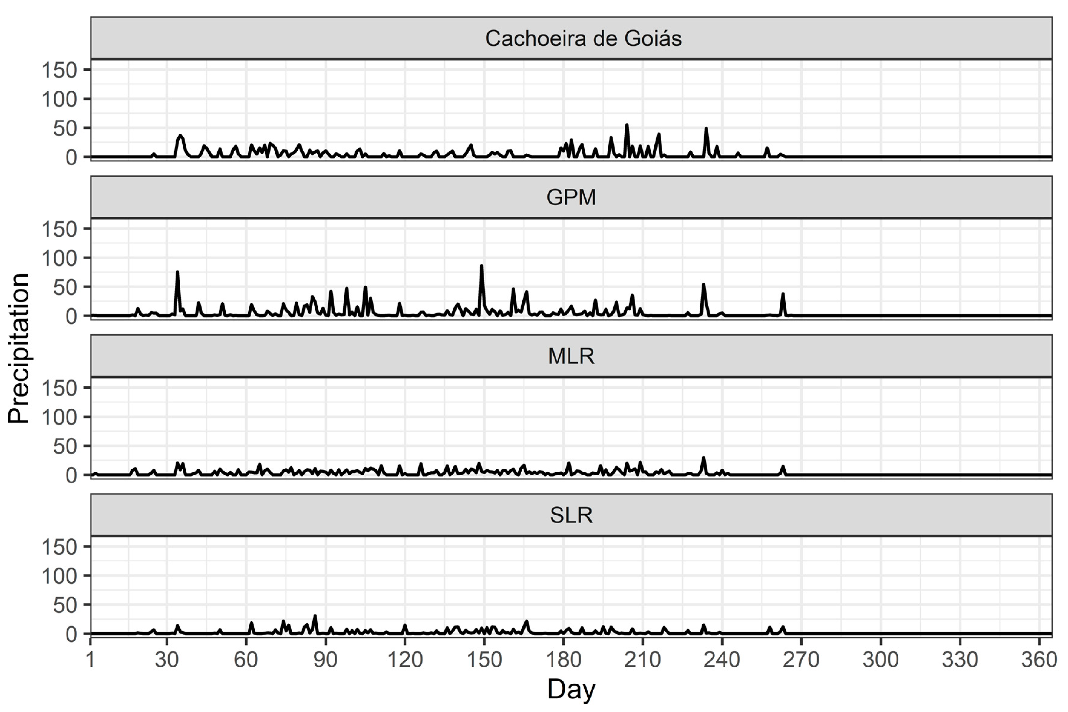
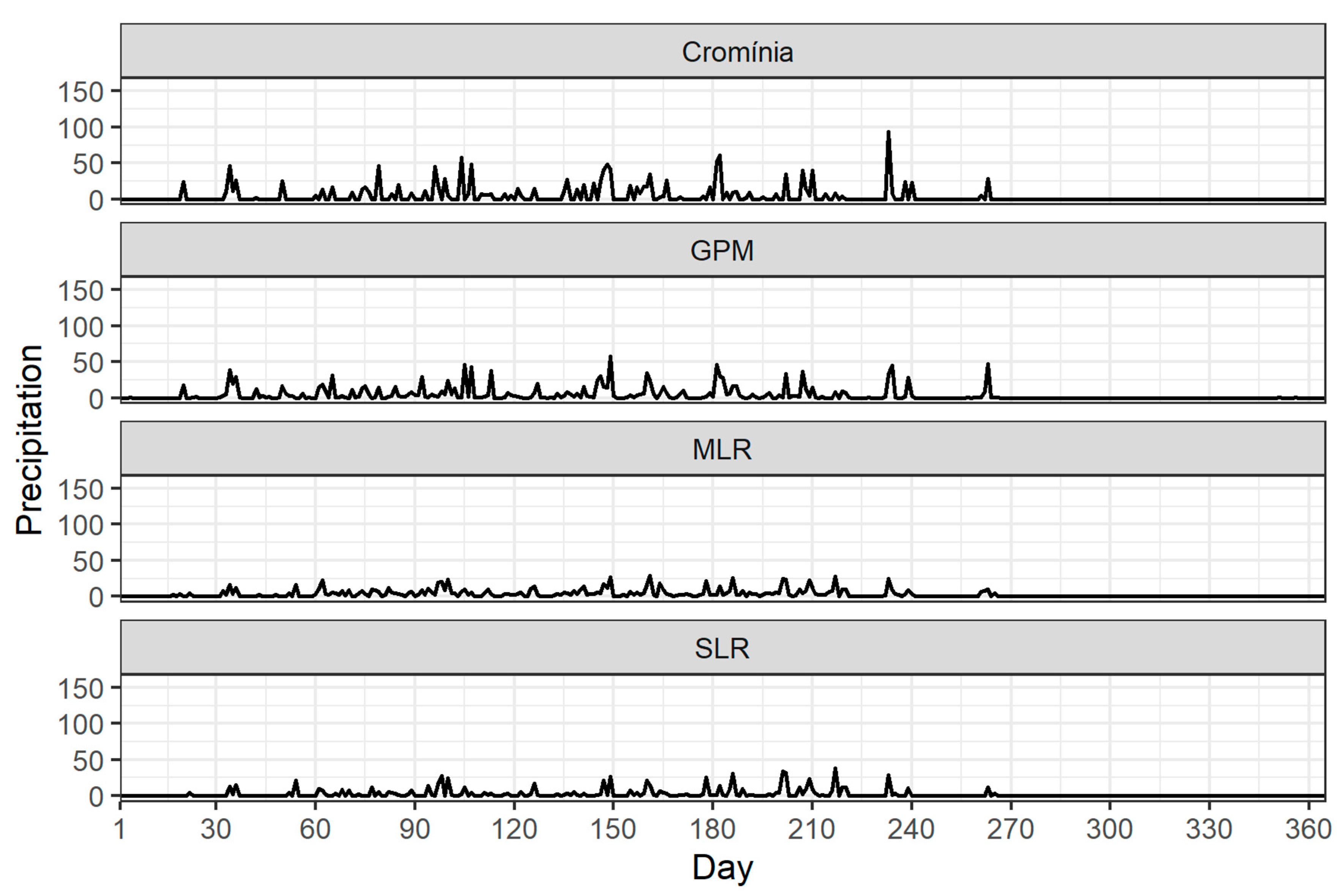
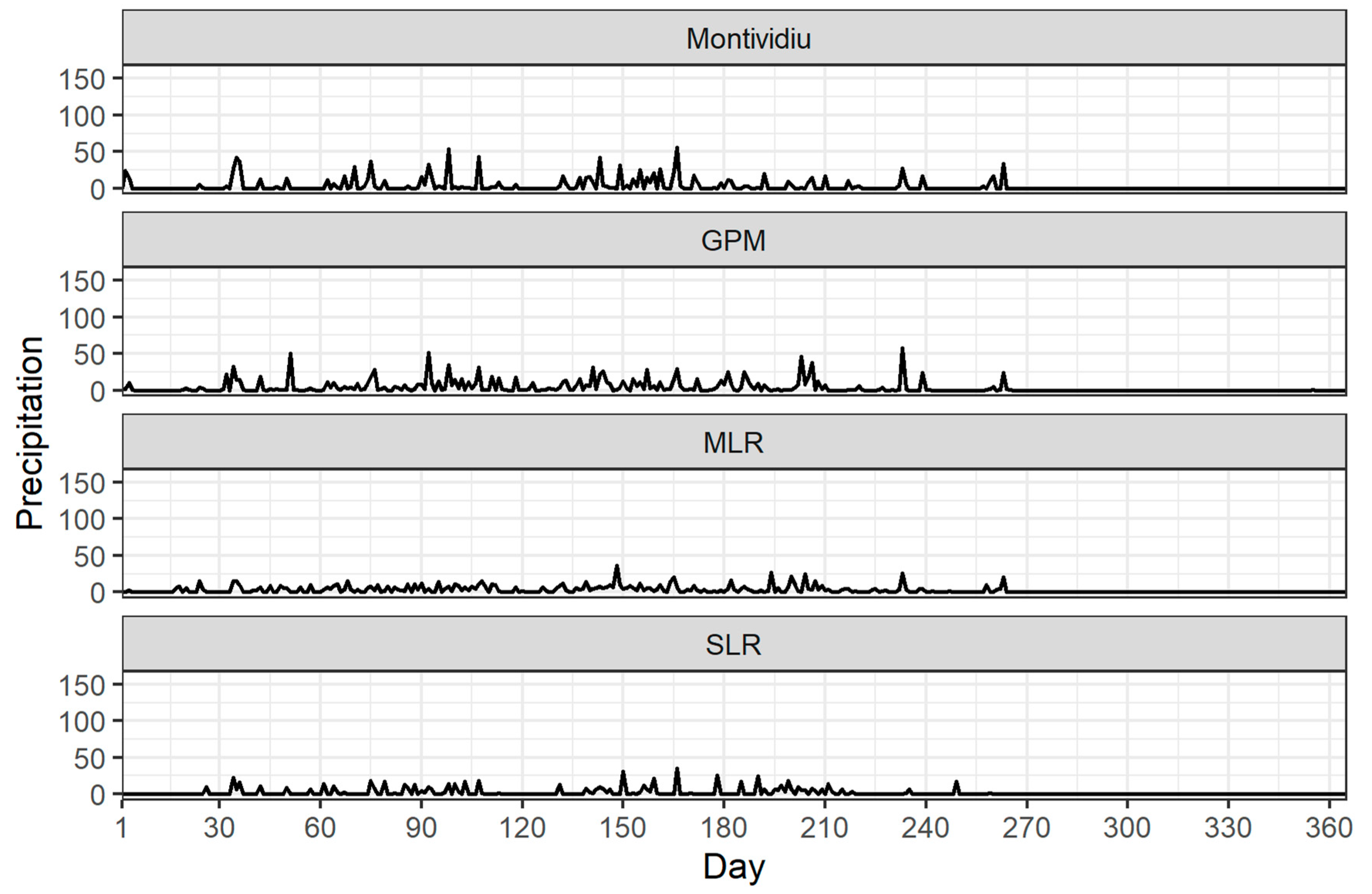
For further analyses, we have also plotted the observed and the estimated time series, as derived from each method for filling missing values, for the testing sites (Figure 4, Figure 5, Figure 6, Figure 7, Figure 8 and Figure 9). One may notice from Figure 4, Figure 5, Figure 6, Figure 7, Figure 8 and Figure 9 that, overall, the “dry state” conditions are poorly represented by the MLR models (remember that the estimates are bounded from below by the equations’ intercepts). In fact, the rainfall amounts estimated with the referred method are, very frequently, much larger than the correspondent intercepts; only the lengthy dry spells, towards the beginning and the end of the water year, were properly captured, as no rainfall was recorded at the “donor” sites. This fact illustrates how the use of fixed “donor” stations may impact the filling of missing values: the complex distribution of storm patterns may induce the frequent imputation of rainfall amounts significantly larger than the lower bounds even when only localized (yet not too small) events are recorded in the vicinities of the target site by one of the “donor” stations. The outlined problem is largely attenuated when the SLR models and the IMERG-GPM retrievals are used, although the latter, to a much lesser extent, still fails in capturing dry spells during some periods of the year. In this case, however, the area-averaged imputed values are closer to zero and the mismatching is probably related to the false alarms from the satellite.
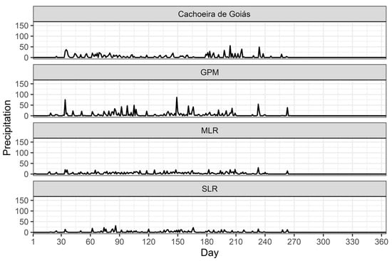
Figure 4.
Direct comparisons between daily precipitation estimates and observed data for the period from 1 September 2016 to 31 August 2016 at the Cachoeira de Goiás station. OBS, observed data; MLR, multiple linear regression method; SLR, simple linear regression; GPM, Global Precipitation Measurement method.
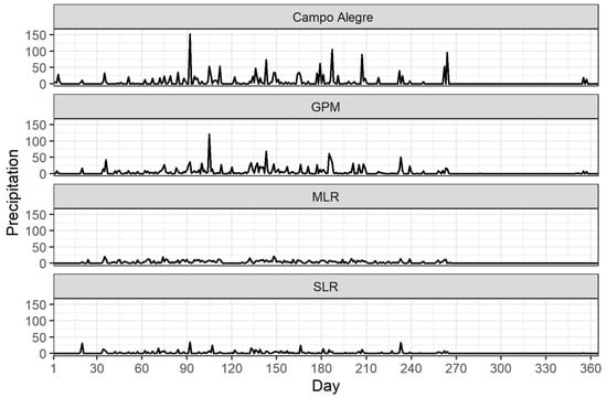
Figure 5.
Direct comparisons between daily precipitation estimates and observed data for the period from 1 September 2016 to 31 August 2016 at the Campo Alegre station. OBS, observed data; MLR, multiple linear regression method; SLR, simple linear regression; GPM, Global Precipitation Measurement method.
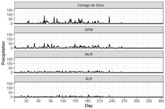
Figure 6.
Direct comparisons between daily precipitation estimates and observed data for the period from 1 September 2016 to 31 August 2016 at the Córrego do Ouro station. OBS, observed data; MLR, multiple linear regression method; SLR, simple linear regression; GPM, Global Precipitation Measurement method.
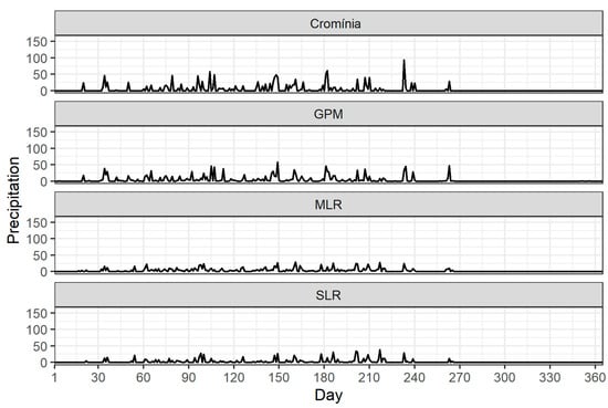
Figure 7.
Direct comparison between daily precipitation estimates and observed data for the period from 1 September 2016 to 31 August 2016 at the Cromínia station. OBS, observed data; MLR, multiple linear regression method; SLR, simple linear regression; GPM, Global Precipitation Measurement method.
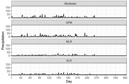
Figure 8.
Direct comparisons between daily precipitation estimates and observed data for the period from 1 September 2016 to 31 August 2016 at the Montividiu station. OBS, observed data; MLR, multiple linear regression method; SLR, simple linear regression; GPM, Global Precipitation Measurement method.
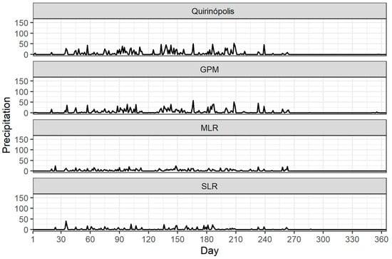
Figure 9.
Direct comparisons between daily precipitation estimates and observed data for the period from 1 September 2016 to 31 August 2016 at the Quirinópolis station. OBS, observed data; MLR, multiple linear regression method; SLR, simple linear regression; GPM, Global Precipitation Measurement method.
Another aspect worth noting in Figure 4, Figure 5, Figure 6, Figure 7, Figure 8 and Figure 9 is that both MLR and SLR models are unable to reproduce the actual patterns of rainfall variability in the target sites. In fact, for most cases, the rainfall amounts appear to be bounded from above at approximately 20 mm and 30 mm for these methods, respectively. As a result, the largest rainfall events are not reproduced by the statistical models, which may justify the larger values of RMSE in most testing stations when such approaches are used for filling missing values. On the other hand, the IMERG-GPM product was able to describe larger rainfall amounts, albeit, due to the spatial averaging across the correspondent pixel; the most extreme events were consistently underestimated by satellite retrievals after downscaling [51]. This condition is more noticeable for the largest events recorded by the gauges, such as those in the Campo Alegre gauging station that exceeded about 70 mm.
Finally, it is clear from Figure 4, Figure 5, Figure 6, Figure 7, Figure 8 and Figure 9 that the temporal dynamics of the largest observed events were best represented by the satellite retrievals and MLR models, whereas, for the SLR counterparts, some lag between observed and estimated rainfall amounts was verified for most cases. Obviously, this may be ascribed to the simplified rationale of SLR models – the timings of the best “donor” station may be different from that of the target site due to storms’ transit along the two gauges. However, for practical purposes, this mismatching may severely impact streamflow estimates derived from continuous rainfall–runoff models as it will affect the water partition among the model components and, accordingly, the rates of runoff production.
3.2. Monthly Estimates
As previously stated, the aggregation of daily data to the monthly scale smooths out the effects of intermittence and rainfall extremes across large areas. As a result, lower levels of variability in the random field (i.e., in the fluctuations around the mean values of the process) are verified in the aggregated process [11] and the performance of statistical methods, with respect to direct imputation of the satellite retrievals, should improve. This conjecture is readily verified in Table 3, which shows the performance indexes of the three methods for filling monthly missing values in the six testing sites. In general, higher levels of linear correlation result at the monthly time scale for all methods. The values of CC were slightly higher for the direct imputation approach (0.90, on average), but, at least with respect to this metric, the MLR models performed just as well (0.89, on average). The GPM product also entailed lower values for MAE (34.6 mm, on average) and RMSE (48.2 mm), with moderate increases in these metrics for the MLR models (37.6 mm for MAE and 53.2 mm for RMSE), but noticeable distinctions for the SLR counterparts (45.3 mm for MAE and 66.7 mm for RMSE). Finally, the underestimation tendencies verified for the regression models, as materialized by the values of PBias, still persist, but to a much lesser extent as compared to the daily time scale (−7.9% for MLR models and −9.9% for SLR models; one should remember that the “donor” sites are different at the daily and the monthly time scales). As for the GPM product, the systematic error amount is again approximately 4% and is mainly driven by the large positive values of PBias in the Cachoeira de Goiás and the Montividiu gauging stations, as discussed in the previous section.

Table 3.
Performance indexes of the three methods for filling monthly missing data at the target sites.
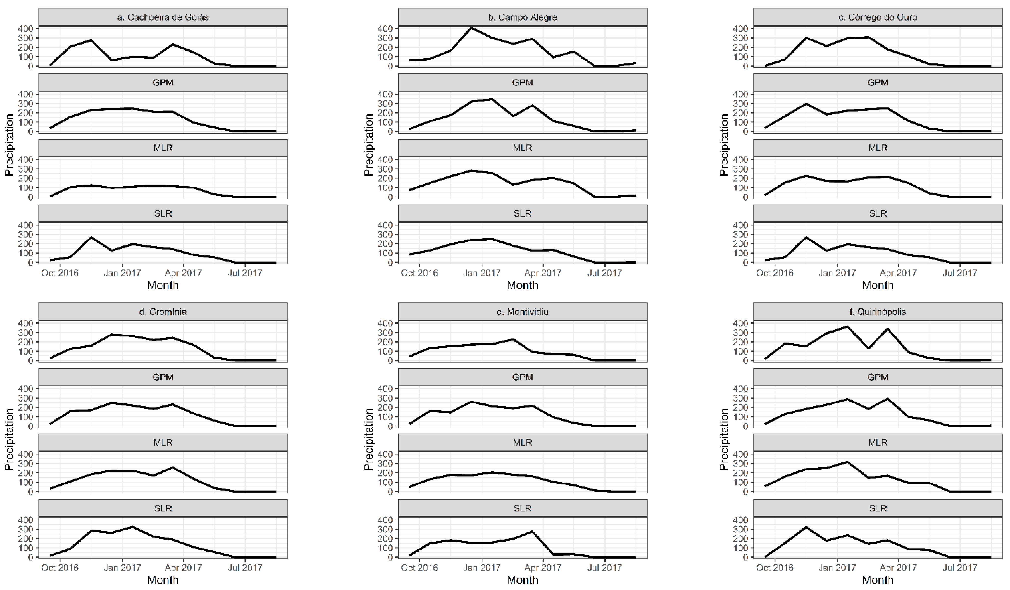
Figure 10 depicts the monthly rainfall time series, as obtained from the gauges and from the models. For ease of visualization, the monthly rainfall amounts are shown as continuous lines (although this representation is conceptually inappropriate). Some general remarks can be made from these plots. First, the MLR estimates are often “oversmoothed”, underestimating the rainfall amounts in the wet season and overestimating otherwise in the testing sites, with the exception of the months of July and August, in which no rainfall was recorded by both the target and the “donor” stations. On the other hand, the SLR estimates did not entail general patterns. In effect, they did provide a reasonable fit in the Montividiu gauging station, with some lack of fit between February and April, but failed to do so at the other target sites, mostly underestimating the recorded rainfall amounts during the dry season. This fact might suggest that the best “donors” for these stations present lower mean annual rainfall amounts or longer dry spells from February to August, as suggested by the relatively lower values of the correlation coefficient, and reinforces our conjecture that the SLR method is, at least for this case study, less effective for filling missing data over a broad range of time scales (day to month).
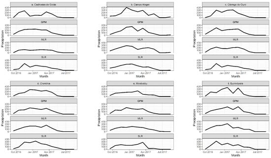
Figure 10.
Monthly precipitation at the test stations: (a) Cachoeira de Goiás, (b) Campo Alegre, (c) Córrego do Ouro, (d) Cromínia, (e) Montividiu, and (f) Quirinópolis in the water year of 2016–2017.
As for the IMERG-GPM product, a tendency of overestimation was observed for most target sites, which is in agreement with the results of [34] for the study region. The seasonal patterns of the observed rainfall were, to some extent, captured in the Córrego do Ouro, the Quirinópolis, and the Montividiu gauging stations, but were grossly misrepresented in the Cachoeira de Goiás (such lack of fit was also observed for the daily time scale). Overall, none of the methods proved able to properly describe the time evolution of monthly rainfall during the water year of 2016–2017. Nonetheless, the goodness of fit assessment in Table 3 and the better agreement with the seasonal features of rainfall, mainly in terms month-to-month variability, as well as the principle of parsimony, seem to suggest that the direct imputation of satellite retrievals is also a more effective alternative for filling missing values in the monthly time scale in our study region.
As compared to previous research efforts at the monthly time scale (e.g., [37,52,53], and references therein), no marked distinctions were found in the performances of the regression-based models, particularly in terms of RMSE and CC, despite the differences in long-term climate conditions in the study regions. Of course, this may be ascribed to the smoother variations of the rainfall fields for the aggregated process, as well as to the smaller degrees of fluctuation around the correspondent mean values at a given site for large time scales [11]. We note, however, the reproduction of seasonal precipitation patterns, which is paramount for drought assessment, is not fully addressed by these studies, which may limit a broader comparison with respect to the overall performance of the regression models. On the other hand, as opposed to the daily time scale, the filling of monthly rainfall with remote-sensing data, after bias correction through a linear model, has been discussed in [36]. Similarly to our results, the referred study concluded that seasonal rainfall patterns are reasonably captured by the satellite retrievals. However, as the satellite estimates are corrected prior to imputation, lower values of RMSE and higher levels of linear correlation were obtained by [36], which again suggests that a bias correction procedure might improve rainfall estimation.
4. Conclusions
This paper discussed the use of statistical-based models and the direct imputation of retrievals from the IMERG-GPM product for filling missing rainfall data in gauging stations located in the Brazilian midwestern region, at daily and monthly time scales. For this, we derived multiple linear regression (MLR) models with fixed “donor” sites and simple linear regression (SLR) models with variable “donor” stations, depending on data availability on the best “donors”, and compared the performance of the three methods, through a set of metrics, by replacing the water year of 2016–2017 with the correspondent estimates.
At the daily time scale, the direct imputation of satellite retrievals provided more accurate results than the statistical-based methods, and described, in a more effective manner, the alternation of dry and wet states of rainfall along the period of evaluation. In effect, the regression models could not capture the spatial variability of complex rainfall fields, which disrupted empirical probability dry at the target sites, and were also unable to reproduce the largest rainfall amounts, being apparently bounded in the range 20–30 mm/day. In addition, at least for this case study, the use of more complex MLR models did not seem justified, as their performance in the goodness-of-fit assessment was similar to those of the more parsimonious SLR models. However, the satellite estimates were biased, mainly with respect to more extreme rainfall events, which might strongly impact frequency analysis expedients. As a result, the adoption of bias-correction procedures (e.g., Ma et al. (2021) [33]) prior to imputation might improve estimation of missing values; this is envisaged as our next research development. Moreover, since the performance of satellite products is inherently dependent on climate and topography [44,54], our results cannot be readily generalized to other regions, although we believe that, at least for time evolution of dry and wet states, remote-sensing data can provide more reliable predictions than the use of “donor” sites. This, however, still calls for further investigation and will be addressed in future work.
On the other hand, the aggregation of the process for deriving monthly data smoothed out the effects of local extremes and intermittence conditions and, as a result, the performance of the statistical-based methods, at least with respect to the metrics utilized in this study, is comparable to those obtained with the direct imputation of satellite retrievals. However, the seasonal precipitation patterns and the month-to-month variability of rainfall amounts were not properly described by the former. This problem is, at least to some extent, attenuated by using remote-sensing data, albeit the IMERG-GPM product could not perform well in all test sites. Moreover, strong tendencies of overestimation were verified in some of the test sites, which reinforces our conjecture that utilizing a bias-correction procedure might improve results, albeit more complex models would result in this case.
To sum up, our results suggest that the imputation of satellite retrievals for filling missing data at times scales ranging from day to month is a feasible alternative and might outperform well-established statistical methods when one is dealing with complex rainfall fields and marked seasonality in precipitation patterns. Of course, the satellite datasets did not span long periods of record, which would certainly limit their use, and more case studies, under a broader variety of climate and terrain complexity conditions, are necessary for providing more general conclusions. However, we believe that the proposed framework may comprise an appealing tool for researchers and practitioners for dealing with missing data in rainfall time series.
Author Contributions
L.V.D. and V.A.F.C. wrote the paper and analyzed the data and the results; K.T.M.F. revised the manuscript and analyzed the results. All authors have read and agreed to the published version of the manuscript.
Funding
This study was financed by Financiadora de Estudos e Projetos (Finep).
Institutional Review Board Statement
Not applicable.
Informed Consent Statement
Not applicable.
Data Availability Statement
Not applicable.
Conflicts of Interest
The authors declare no conflict of interest.
References
- Kidd, C.; Bauer, P.; Turk, J.; Huffman, G.J.; Joyce, R.; Hsu, K.-L.; Braithwaite, D. Intercomparison of High-Resolution Precipitation Products over Northwest Europe. J. Hydrometeorol. 2012, 13, 67–83. [Google Scholar] [CrossRef]
- Danelichen, V.H.D.M.; Machado, N.G.; Biudes, M.S.; Souza, M.C. TRMM Satellite Performance in Estimated Rainfall over the Midwest Region of Brazil. Revista Brasileira de Climatologia 2013, 12, 22–31. [Google Scholar] [CrossRef][Green Version]
- Santana, A.; Soares, D. Avaliação Das Estimativas de Chuva Do Satélite TRMM No Estado Da Paraíba. Revista Brasileira de Recursos Hídricos 2016, 21, 288–299. [Google Scholar]
- Vicente-Serrano, S.M.; Beguería, S.; Lopez-Moreno, I.; Vera, M.G.; Stepanek, P. A complete daily precipitation database for northeast Spain: Reconstruction, quality control, and homogeneity. Int. J. Clim. 2009, 30, 1146–1163. [Google Scholar] [CrossRef]
- Falck, A.S.; Maggioni, V.; Tomasella, J.; Vila, D.A.; Diniz, F.L. Propagation of satellite precipitation uncertainties through a distributed hydrologic model: A case study in the Tocantins–Araguaia basin in Brazil. J. Hydrol. 2015, 527, 943–957. [Google Scholar] [CrossRef]
- Nóbrega, R.S.; de Souza, Ê.P.; Galvíncio, J.D. Análise Da Estimativa De Precipitação Do Trmm Em Uma Sub-Bacia Da Amazônia Ocidental. Revista de Geografia-Recife 2008, 25, 6–20. [Google Scholar]
- Wagner, P.D.; Fiener, P.; Wilken, F.; Kumar, S.; Schneider, K. Comparison and evaluation of spatial interpolation schemes for daily rainfall in data scarce regions. J. Hydrol. 2012, 464–465, 388–400. [Google Scholar] [CrossRef]
- Wai, K.; Che, C. A Comparative Analysis of Soft Computing Techniques Used to Estimate Missing Precipitation Records. In Proceedings of the 19th Biennial Conference of the International Telecommunications Society (ITS), Bangkok, Thailand, 18–21 November 2012; pp. 18–21. [Google Scholar]
- de Oliveira, L.F.C.; Antonini, J.C.A.; Fioreze, A.P.; Silva, M.A.S. Métodos de Estimativa de Precipitação Máxima Para o Estado de Goiás Maximum Rainfall Estimation Methods for Goiás. Revista Brasileira de Engenharia Agrícola e Ambiental 2008, 12, 620–625. [Google Scholar] [CrossRef]
- de Oliveira, L.F.C.; Antonini, J.C.D.A.; Griebeler, N.P. Estimativas de chuvas intensas para o Estado de Goiás. Engenharia Agrícola 2008, 28, 22–33. [Google Scholar] [CrossRef]
- Koutsoyiannis, D. Stochastics of Hydroclimatic Extremes, 1st ed.; Barouxis, C., Ed.; Kallipos: Athens, Greece, 2021. [Google Scholar]
- Costa, V.; Silva, A.; Palmier, L.R.; Sampaio, J. Assessing the Propagation from Meteorological to Hydrological Drought in the São Francisco River Catchment with Standardized Indexes: Exploratory Analysis, Influential Factors, and Forecasting Strategies. J. Water Resour. Plan. Manag. 2021, 147, 05021020. [Google Scholar] [CrossRef]
- Costa, V.; Fernandes, W. Bayesian estimation of extreme flood quantiles using a rainfall-runoff model and a stochastic daily rainfall generator. J. Hydrol. 2017, 554, 137–154. [Google Scholar] [CrossRef]
- Pappas, C. A Quick Gap-filling of Missing Hydrometeorological Data. J. Geophys. 2014, 119, 1–11. [Google Scholar] [CrossRef]
- de Oliveira, L.F.C.; Fioreze, A.P.; Medeiros, A.M.M.; Silva, M.A.S. Comparison of Gap Filling Methodologies of Annual Historical Series of Rainfall. Revista Brasileira de Engenharia Agrícola e Ambiental 2010, 14, 1186–1192. [Google Scholar] [CrossRef]
- Strachan, S.; Kelsey, E.P.; Brown, R.F.; Dascalu, S.; Harris, F.; Kent, G.; Lyles, B.; Mccurdy, G.; Slater, D.; Smith, K.; et al. Technology, Refined Instrument Siting, and a Focus on Gradients Filling the Data Gaps in Mountain Climate Observatories Through Advanced Technology, Refined Instrument Siting, and a Focus on Gradients. Mt. Res. Dev. 2016, 36, 518–527. [Google Scholar] [CrossRef]
- Teegavarapu, R.S.; Chandramouli, V. Improved weighting methods, deterministic and stochastic data-driven models for estimation of missing precipitation records. J. Hydrol. 2005, 312, 191–206. [Google Scholar] [CrossRef]
- Borga, M.; Vizzaccaro, A. On the interpolation of hydrologic variables: Formal equivalence of multiquadratic surface fitting and kriging. J. Hydrol. 1997, 195, 160–171. [Google Scholar] [CrossRef]
- Kizza, M.; Westerberg, I.; Rodhe, A.; Ntale, H.K. Estimating areal rainfall over Lake Victoria and its basin using ground-based and satellite data. J. Hydrol. 2012, 464–465, 401–411. [Google Scholar] [CrossRef]
- Plouffe, C.C.; Robertson, C.; Chandrapala, L. Comparing interpolation techniques for monthly rainfall mapping using multiple evaluation criteria and auxiliary data sources: A case study of Sri Lanka. Environ. Model. Softw. 2015, 67, 57–71. [Google Scholar] [CrossRef]
- Bertoni, J.C.; Tucci, C.E.M. Precipitação. In Hidrologia: Ciência e Aplicação; Tucci, C.E.M., Ed.; ABRH: Porto Alegre, Brazil, 2007; Volume 4, pp. 177–241. [Google Scholar]
- Bennett, N.D.; Newham, L.T.H.; Croke, B.F.W.; Jakeman, A.J. Patching and Disaccumulation of Rainfall Data for Hydrological Modelling. In Proceedings of the International Congress on Modelling and Simulation (MODSIM 2007), Christchurch, New Zealand, 10–13 December 2007; pp. 2520–2526. [Google Scholar]
- Hasana, M.; Crokea, B. Filling Gaps in Daily Rainfall Data: A Statistical Approach. In Proceedings of the 20th International Congress on Modelling and Simulation, Adelaide, Australia, 1–6 December 2013; pp. 1–6. [Google Scholar]
- Simolo, C.; Brunetti, M.; Maugeri, M.; Nanni, T. Improving estimation of missing values in daily precipitation series by a probability density function-preserving approach. Int. J. Clim. 2009, 30, 1564–1576. [Google Scholar] [CrossRef]
- Nathans, L.; Oswald, F.; Nimon, K. Interpreting Multiple Linear Regression: A Guidebook of Variable Importance. Pract. Assesment Res. Eval. 2012, 17, 19. [Google Scholar] [CrossRef]
- Lebay, M.; Le, M. Techniques of Filling Missing Values of Daily and Monthly Rain Fall Data: A Review. SF J. Environ. Earth Sci. 2020, 3, 1036. [Google Scholar]
- Portuguez-Maurtua, M.; Arumi, J.L.; Lagos, O.; Stehr, A.; Arquiñigo, N.M. Filling Gaps in Daily Precipitation Series Using Regression and Machine Learning in Inter-Andean Watersheds. Water 2022, 14, 1799. [Google Scholar] [CrossRef]
- Körner, P.; Kronenberg, R.; Genzel, S.; Bernhofer, C. Introducing Gradient Boosting as a universal gap filling tool for meteorological time series. Meteorol. Z. 2018, 27, 369–376. [Google Scholar] [CrossRef]
- Kim, J.; Ryu, J.H. Quantifying a Threshold of Missing Values for Gap Filling Processes in Daily Precipitation Series. Water Resour. Manag. 2015, 29, 4173–4184. [Google Scholar] [CrossRef]
- Brocca, L.; Ciabatta, L.; Massari, C.; Moramarco, T.; Hahn, S.; Hasenauer, S.; Levizzani, V. Soil as a naturalrain gauge: Estimating global rainfallfrom satellite soil moisture data. J. Geophys. Res. Atmos. 2014, 119, 5128–5141. [Google Scholar] [CrossRef]
- Huffman, G.J.; Bolvin, D.T.; Nelkin, E.J.; Wolff, D.B.; Adler, R.F.; Gu, G.; Hong, Y.; Bowman, K.P.; Stocker, E.F. The TRMM Multisatellite Precipitation Analysis (TMPA): Quasi-Global, Multiyear, Combined-Sensor Precipitation Estimates at Fine Scales. J. Hydrometeorol. 2007, 8, 38–55. [Google Scholar] [CrossRef]
- Seyyedi, H.; Anagnostou, E.N.; Kirstetter, P.-E.; Maggioni, V.; Hong, Y.; Gourley, J.J. Incorporating Surface Soil Moisture Information in Error Modeling of TRMM Passive Microwave Rainfall. IEEE Trans. Geosci. Remote Sens. 2014, 52, 6226–6240. [Google Scholar] [CrossRef]
- Ma, Y.; Sun, X.; Chen, H.; Hong, Y.; Zhang, Y. A two-stage blending approach for merging multiple satellite precipitation estimates and rain gauge observations: An experiment in the northeastern Tibetan Plateau. Hydrol. Earth Syst. Sci. 2021, 25, 359–374. [Google Scholar] [CrossRef]
- Duarte, L.V.; Formiga, K.T.M.; Costa, V.A.F. Analysis of the IMERG-GPM Precipitation Product Analysis in Brazilian Midwestern Basins Considering Different Time and Spatial Scales. Water 2022, 14, 2472. [Google Scholar] [CrossRef]
- Siabi, N.; Sanaeinejad, S.H.; Ghahraman, B. Comprehensive evaluation of a spatio-temporal gap filling algorithm: Using remotely sensed precipitation, LST and ET data. J. Environ. Manag. 2020, 261, 110228. [Google Scholar] [CrossRef]
- Cordeiro, A.L.D.M.; Blanco, C.J.C. Assessment of satellite products for filling rainfall data gaps in the Amazon region. Nat. Resour. Model. 2021, 34, e12298. [Google Scholar] [CrossRef]
- Abu Romman, Z.; Al-Bakri, J.; Al Kuisi, M. Comparison of methods for filling in gaps in monthly rainfall series in arid regions. Int. J. Clim. 2021, 41, 6674–6689. [Google Scholar] [CrossRef]
- PRODUTO 5: Plano Estadual de Recursos Hídricos Revisão Final-Setembro 2015. Available online: https://www.meioambiente.go.gov.br/images/imagens_migradas/upload/arquivos/2016-01/p05_plano_estadual_de_recursos_hidricos_revfinal2016.pdf (accessed on 5 July 2022).
- Matsui, T.; Tao, W.; Munchak, S.J.; Grecu, M.; Huffman, G.J. Satellite view of quasi-equilibrium states in tropical convection and precipitation microphysics. Geophys. Res. Lett. 2015, 42, 1959–1968. [Google Scholar] [CrossRef]
- Tabony, R.C. The estimation of missing climatological data. J. Clim. 1983, 3, 297–314. [Google Scholar] [CrossRef]
- Costa, V. Correlation and Regression. In Fundamentals of Statistical Hydrology; Springer International Publishing: Cham, Switzerland, 2017; pp. 391–440. [Google Scholar]
- Xu, G.; Xu, X.; Liu, M.; Sun, A.Y.; Wang, K. Spatial Downscaling of TRMM Precipitation Product Using a Combined Multifractal and Regression Approach: Demonstration for South China. Water 2015, 7, 3083–3102. [Google Scholar] [CrossRef]
- Kim, K.; Park, J.; Baik, J.; Choi, M. Evaluation of topographical and seasonal feature using GPM IMERG and TRMM 3B42 over Far-East Asia. Atmospheric Res. 2017, 187, 95–105. [Google Scholar] [CrossRef]
- Tang, G.; Long, D.; Hong, Y.; Gao, J.; Wan, W. Documentation of multifactorial relationships between precipitation and topography of the Tibetan Plateau using spaceborne precipitation radars. Remote Sens. Environ. 2018, 208, 82–96. [Google Scholar] [CrossRef]
- Oliveira, P.T.S.; Nearing, M.A.; Moran, M.S.; Goodrich, D.C.; Wendland, E.; Gupta, H.V. Trends in water balance components across the Brazilian Cerrado. Water Resour. Res. 2014, 50, 7100–7114. [Google Scholar] [CrossRef]
- Papailiou, I.; Spyropoulos, F.; Trichakis, I.; Karatzas, G.P. Artificial Neural Networks and Multiple Linear Regression for Filling in Missing Daily Rainfall Data. Water 2022, 14, 2892. [Google Scholar] [CrossRef]
- Aieb, A.; Madani, K.; Scarpa, M.; Bonaccorso, B.; Lefsih, K. A new approach for processing climate missing databases applied to daily rainfall data in Soummam watershed, Algeria. Heliyon 2019, 5, e01247. [Google Scholar] [CrossRef] [PubMed]
- Camuffo, D.; Becherini, F.; della Valle, A.; Zanini, V. A comparison between different methods to fill gaps in early precipitation series. Environ. Earth Sci. 2022, 81, 1–14. [Google Scholar] [CrossRef]
- Kim, J.; Ryu, J.H. A Heuristic Gap Filling Method for Daily Precipitation Series. Water Resour. Manag. 2016, 30, 2275–2294. [Google Scholar] [CrossRef]
- Grillakis, M.G.; Polykretis, C.; Manoudakis, S.; Seiradakis, K.D.; Alexakis, D.D. A Quantile Mapping Method to Fill in Discontinued Daily Precipitation Time Series. Water 2020, 12, 2304. [Google Scholar] [CrossRef]
- Chen, F.; Gao, Y.; Wang, Y.; Qin, F.; Li, X. Downscaling satellite-derived daily precipitation products with an integrated framework. Int. J. Clim. 2018, 39, 1287–1304. [Google Scholar] [CrossRef]
- Farzandi, M.; Sanaeinejad, H.; Rezaei-Pazhan, H.; Sarmad, M. Improving estimation of missing data in historical monthly precipitation by evolutionary methods in the semi-arid area. Environ. Dev. Sustain. 2021, 24, 8313–8332. [Google Scholar] [CrossRef]
- Sattari, M.T.; Rezazadeh-Joudi, A.; Kusiak, A. Assessment of different methods for estimation of missing data in precipitation studies. Hydrol. Res. 2016, 48, 1032–1044. [Google Scholar] [CrossRef]
- Amjad, M.; Yilmaz, M.T.; Yucel, I.; Yilmaz, K.K. Performance evaluation of satellite- and model-based precipitation products over varying climate and complex topography. J. Hydrol. 2020, 584, 124707. [Google Scholar] [CrossRef]
Publisher’s Note: MDPI stays neutral with regard to jurisdictional claims in published maps and institutional affiliations. |
© 2022 by the authors. Licensee MDPI, Basel, Switzerland. This article is an open access article distributed under the terms and conditions of the Creative Commons Attribution (CC BY) license (https://creativecommons.org/licenses/by/4.0/).


