A Daily Water Balance Model Based on the Distribution Function Unifying Probability Distributed Model and the SCS Curve Number Method

Abstract

A new daily water balance model is developed and tested in this paper. The new model has a similar model structure to the existing probability distributed rainfall runoff models (PDM), such as HyMOD. However, the model utilizes a new distribution function for soil water storage capacity, which leads to the SCS (Soil Conservation Service) curve number (CN) method when the initial soil water storage is set to zero. Therefore, the developed model is a unification of the PDM and CN methods and is called the PDM–CN model in this paper. Besides runoff modeling, the calculation of daily evaporation in the model is also dependent on the distribution function, since the spatial variability of soil water storage affects the catchment-scale evaporation. The generated runoff is partitioned into direct runoff and groundwater recharge, which are then routed through quick and slow storage tanks, respectively. Total discharge is the summation of quick flow from the quick storage tank and base flow from the slow storage tank. The new model with 5 parameters is applied to 92 catchments for simulating daily streamflow and evaporation and compared with AWMB, SACRAMENTO, and SIMHYD models. The performance of the model is slightly better than HyMOD but is not better compared with the 14-parameter model (SACRAMENTO) in the calibration, and does not perform as well in the validation period as the 7-parameter model (SIMHYD) in some areas, based on the NSE values. The linkage between the PDM–CN model and long-term water balance model is also presented, and a two-parameter mean annual water balance equation is derived from the proposed PDM–CN model.

1. Introduction

Conceptual water balance models have been used to simulate and predict hydrological variables (e.g., runoff, evaporation, and storage change) for many applications, such as reservoir operations and climate change impact assessments. Various conceptual daily water balance models have been developed in the literature. Usually, models are developed to meet specific conditions of hydrologic and climatic areas, and using them for purposes other than their created purpose will result in unsatisfactory results [1]. Many models, as an example, have depicted poor simulations for minimum flow situations; in that respect, the representation of hydrological process will depend on how relevant models are developed to meet low-flow conditions [2,3]. Conceptual models have their advantages and disadvantages. They can predict and simulate hydrological processes for decision making [4,5,6,7,8], prediction of streamflow in ungauged watersheds [9,10,11,12,13], evaluating changes of land use [14,15,16,17], evaluating climate change implications [18,19,20,21], and evaluating human impacts [4,22,23]. Despite their advantages, hydrological models can have limitations in considering groundwater exchange, in oversimplifying hydrological processes, or in their underestimating of the importance of simulated water balance [1]. Schaake, et al. [22] developed a five-parameter daily water balance model and found that the model is favorably comparable to the more sophisticated Sacramento soil moisture accounting (SAC-SMA) model [23]. Zhang, et al. [24] developed a dynamic water balance model, based on the Budyko framework [25], for multiple time scales, including the daily scale. Particularly, the lumped conceptual model, HyMOD [26,27], with five parameters, has been used in many studies, such as in the performance evaluation of model calibration algorithms (e.g., [26,27,28,29,30,31]). The HyMOD has been utilized to predict streamflow and model calibration. Parra, Fuentes-Aguilera and Muñoz [1] described that HyMOD uses rainfall excess with five parameters: maximum soil moisture capacity ($FC$) and degree of soil moisture spatial variability $(\beta$) [27]. Then, an excess of precipitation is controlled by $\left(\alpha \right)$ and directed to quick flow reservoir with residence time $\left(K_q\right)$, generating quick flow $\left(Q_f\right)$, having a quick flow tank. The rest of the rainfall excess $\left(1-\alpha \right)$ is then directed to slow flow $\left(Q_S\right)$ with residence time $\left(K_s\right)$, having a slow flow tank. The sum of both quick flow and slow flow generates the total streamflow of a watershed.

As a probability distributed model (PDM) for rainfall runoff [32], the runoff generation of the HyMOD model is based on a generalized Pareto distribution for describing spatial variability of soil water storage capacity. The generalized Pareto distribution has been used in many saturation excess runoff generation models, such as the Xinanjiang model [32,33,34], the VIC model [35,36], and the ARNO model [37]. The generated runoff in the HyMOD model is partitioned into direct runoff and groundwater recharge, which are then routed through quick and slow storage tanks, respectively. Evaporation is computed as the lower value between potential evaporation and soil water storage [26].

Besides PDM, runoff has also been modeled by empirical equations, such as the Soil Conservation Service curve number (SCS–CN) method [38]. The SCS–CN method has been extensively used for modeling surface runoff in engineering hydrology community and many hydrologic models such as HEC-HMS [39], HSPF [40], and SWAT [41]. The SCS–CN method has been interpreted as an infiltration excess runoff model [42,43,44,45], as well as a saturation excess runoff model [46,47,48,49]. The SCS–CN method was originally developed for runoff calculation at the event scale and the effect of antecedent soil moisture condition is not explicitly represented in the runoff equation [50]. The implicit representation of initial soil moisture condition in the SCS–CN method causes a challenge for applying the SCS–CN method to continuous simulation of water balance [44,51].

Recently, Wang [52] proposed a new distribution function for describing the spatial variability of soil water storage capacity, and the corresponding runoff equation becomes the SCS–CN method when the initial soil water storage is set to zero. Therefore, the new distribution unifies the runoff calculation of the SCS–CN method and PDM such as HyMOD. The new distribution function can be used to replace the generalized Pareto distribution in PDM or saturation excess runoff models. This will provide a linkage between saturation excess runoff models and the SCS–CN method. For example, the average soil water storage capacity of a catchment is related to the curve number, which is estimated based on available land cover and soil data. Meanwhile, the issue of implicit representation of initial soil moisture condition in the SCS–CN method is resolved automatically, since the soil moisture carryover is accounted in PDM.

The objective of this paper is to develop a daily water balance model (called PDM–CN), based on the new distribution function for soil water storage capacity. The daily water balance model has the similar model structure as the HyMOD model. The differences between the developed PDM–CN model and the HyMOD model include the following: (1) the new distribution function is used for soil water storage capacity by replacing the generalized Pareto distribution; (2) the calculation of evaporation is also based on the distribution function in the PDM–CN model. The developed daily water balance model is described in Section 2. The study catchments for the application of the model are introduced in Section 3. Results and discussions are presented in Section 4, and conclusions are summarized in Section 5.

2. Description of the Daily Water Balance Model

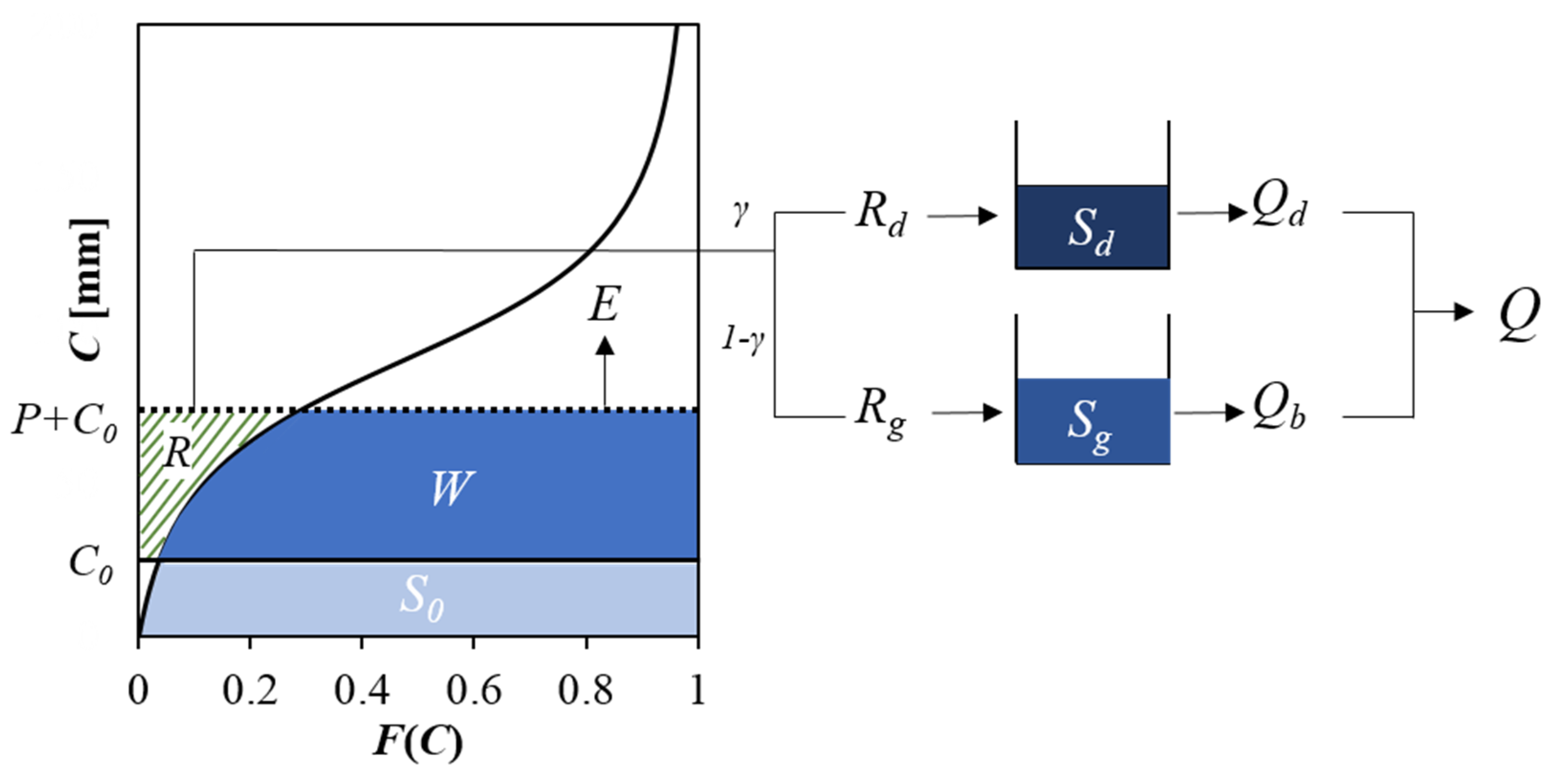
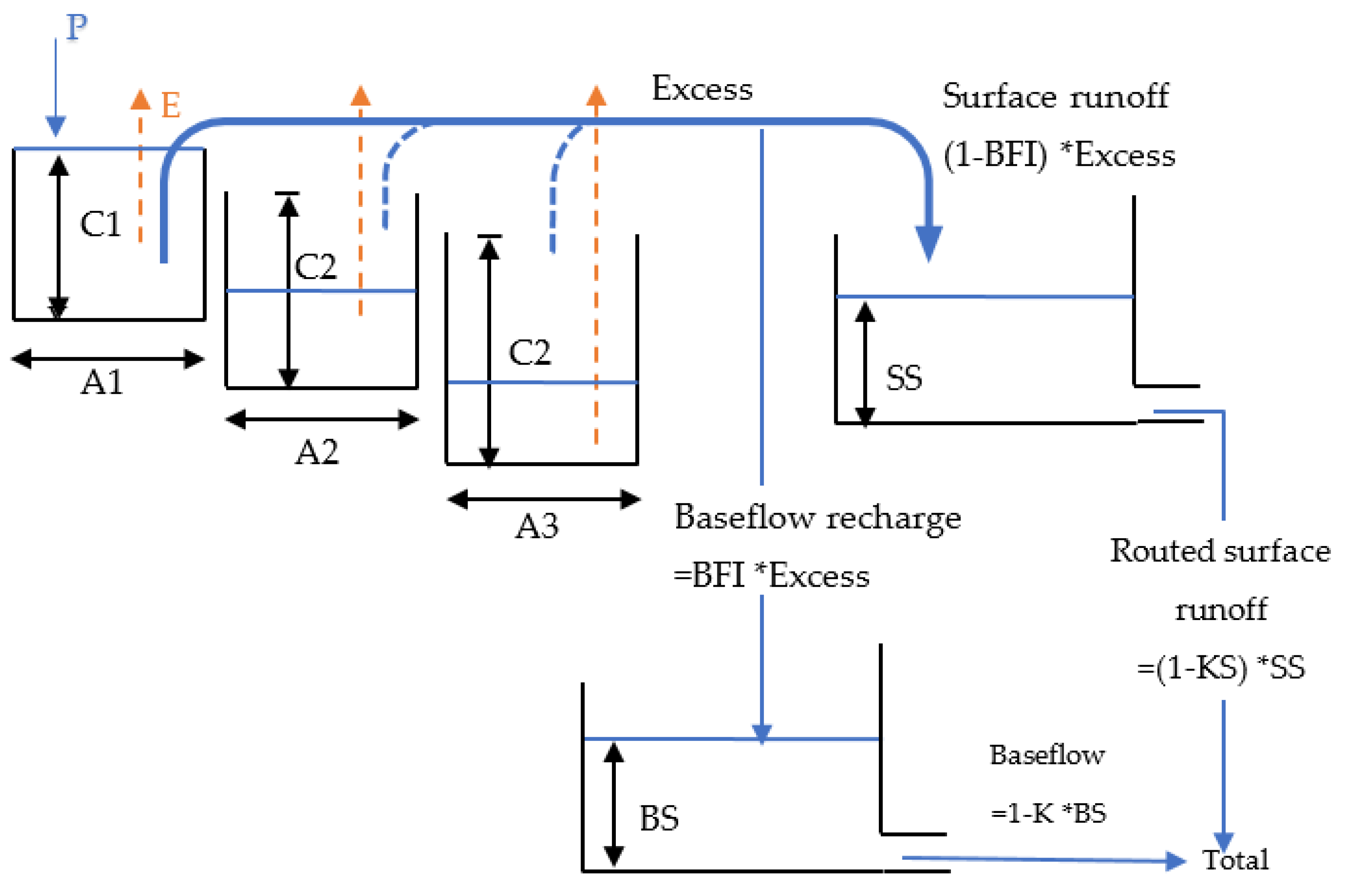
The developed daily water balance model is described in this section. The model structure is similar to the HyMOD model, as shown in Figure 1. Soil wetting (i.e., infiltration) and runoff are computed based on the distribution function describing the spatial variability of soil water storage capacity. Evaporation is computed as a function of soil water storage and potential evaporation. Runoff is partitioned into direct runoff and groundwater recharge. Direct runoff is routed through a quick storage tank, from which the release is quick flow. Groundwater recharge is routed through a slow storage tank, from which the release is base flow. The summation of quick flow and base flow is the total discharge. The ranges of parameters used for calibration for the HyMOD are also listed in Table 1.

Figure 1. The structure of the proposed PDM–CN model which unifies the PDM (probability distributed model) and the SCS curve number method.

Table 1. The ranges of parameters for the proposed PDM–CN model and HyMOD model.

PDM–CN Model			HyMOD
Parameter	Range	Unit	Parameter	Range	Unit
$a$	0.01–2	-	$\beta$	0.01–7	-
$S_b$	50–1500	mm	$C_{max}$	50–2000	mm
$\gamma$	0.01–1	-	${\gamma }_2$	0.01–1	-
$k_d$	0.14–1	day−1	$k_{d2}$	0.14–1	day−1
$k_b$	0.01–0.14	day−1	$k_{b2}$	0.01–0.14	day−1

2.1. Soil Wetting

The spatial variation of point-scale storage capacity (C) is represented by the following cumulative distribution function (CDF), proposed by [52]:

$$F\left(C\right)=1-\frac{1}{a}+\frac{C+\left(1-a\right)S_b}{a\sqrt{{\left(C+S_b\right)}^2-2a{S}_{b}C}}$$

(1)

where C is soil water storage capacity at a point, and it is supported by a positive semi-infinite interval (i.e., $C\ge 0$); $F\left(C\right)$ is the fraction of the catchment in Equation (1) area for which the storage capacity is less than C; $a$ is the shape parameter with a range of $0<a<2$; $S_b$ is the mean of the distribution, i.e., the average soil water storage capacity over the catchment. As discussed earlier, the generalized Pareto distribution is used in the HyMOD model as well as VIC model. The differences between these two distribution functions are discussed by Wang [52,53].

As shown in Figure 1, the initial average soil moisture is denoted as $S_0$, and the corresponding value of $C$ is denoted as $C_0$. The precipitation depth ($P$) is partitioned into a runoff ($R$) and soil wetting ($W$) (i.e., infiltration). Soil wetting is computed by the following integration [27]:

$$W={{\displaystyle \int }}_{C_0}^{P+C_0}\left(1-F\right)dC$$

(2)

Substituting Equation (1) into Equation (2), soil wetting is obtained [52], as follows:

$$W=\frac{P+S_b\sqrt{{\left(m+1\right)}^2-2am}-\sqrt{{\left[P+\left(m+1\right)S_b\right]}^2-2am{S}_b{}^2-2a{S}_{b}P}}{a}$$

(3)

where,

$$m=\frac{S_0\left(2S_b-a{S}_0\right)}{2\left(S_b-S_0\right)}$$

(4)

If initial soil water storage is zero (i.e., $S_0=0$), Equation (4) becomes the proportionality relationship of the SCS–CN method [52]. Therefore, the computation of soil wetting by Equation (3) is an extension of the SCS–CN method by incorporating initial soil moisture explicitly. Therefore, the developed daily model is called PDM–CN.

2.2. Evaporation

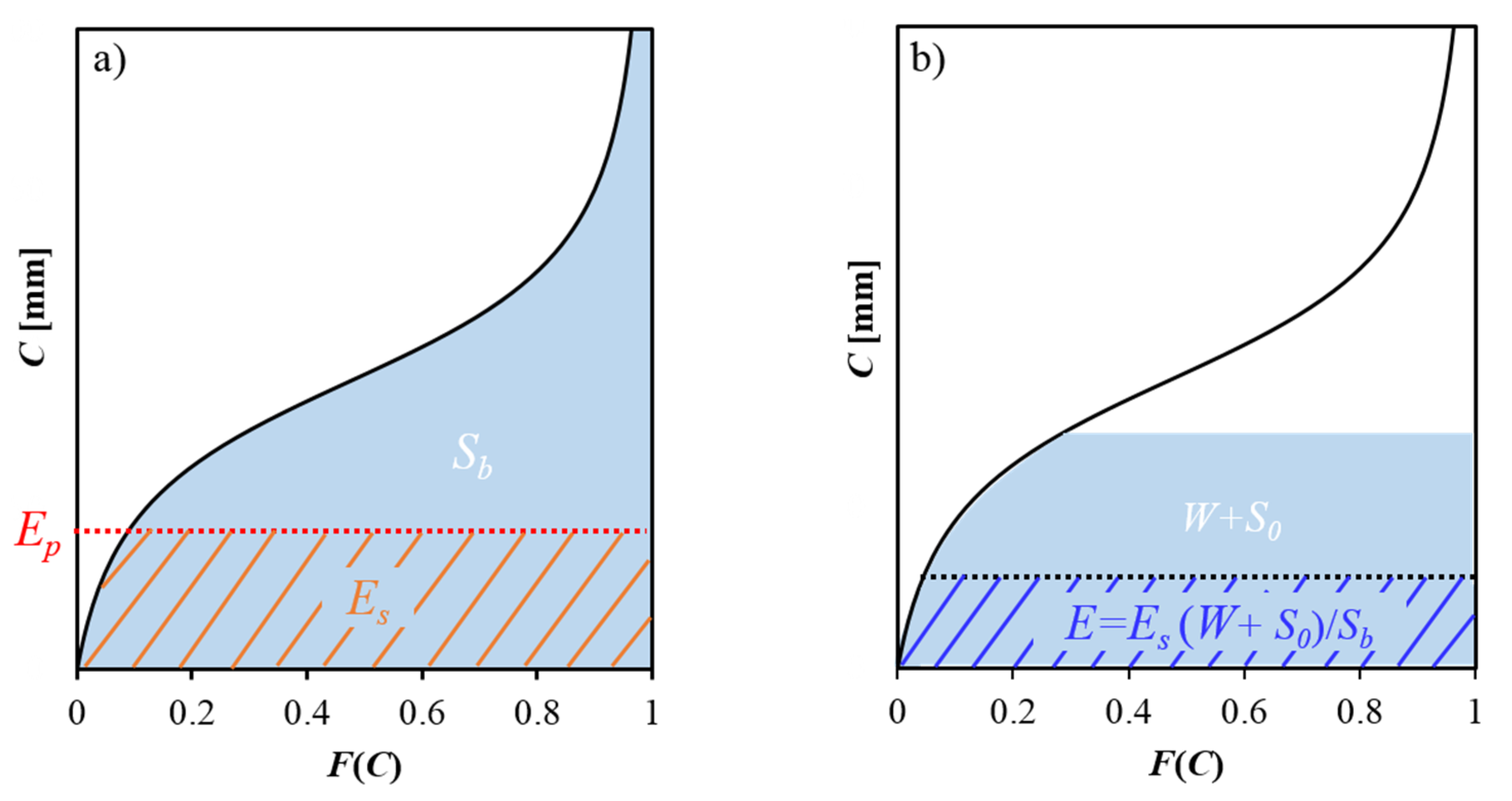
Once $W$ is computed by Equation (3), the sum of soil wetting and initial soil water storage is computed as $Y=W+S_0$. $Y$ is then partitioned into evaporation ($E$) and ending soil water storage ($S_1)$, i.e., $Y=E+S_1$. In the HyMOD model, $E$ is computed as the smaller value between $Y$ and potential evaporation ($E_P$), i.e., $E=\min \left(Y,E_P\right)$. However, the computation of evaporation in the proposed PDM–CN model considers the spatial variability of soil water storage in Equation (5). As shown in Figure 1, the actual soil water storage varies spatially due to the spatial variability of storage capacity. Therefore, the actual evaporation also varies spatially even though the potential evaporation is spatially uniform. As shown in Figure 2a, when the soil water storage at every point in a catchment reaches their storage capacities (i.e., the entire catchment is saturated), the average evaporation over the entire catchment is computed as follows:

$$E_s={{\displaystyle \int }}_0^{E_P}\left(1-F\left(C\right)\right)dC$$

(5)

Figure 2. The calculation of evaporation for two cases: (a) the entire catchment is saturated; (b) the catchment is partially saturated.

As demonstrated in Figure 2a, $E_s$ is smaller than $E_P$, even though the average storage ($S_b)$ is higher than $E_P$. The reason is that the soil water storage at some points is lower than $E_P$ and evaporation at those points is equal to the corresponding soil water storage. $E_s$ is spatially averaged evaporation for the condition that the entire catchment is saturated in Equation (6). For the condition when the entire catchment is not saturated with average storage of $W+S_0$, evaporation is reduced from $E_s$ proportionally to the relative soil water storage (Figure 2b), as follows:

$$E=\frac{W+S_0}{S_b}{E}_s$$

(6)

Therefore, evaporation is computed after substituting Equation (1) into Equation (5), as resulted in Equation (7), as follows:

$$E=\frac{W+S_0}{S_b}\frac{E_P+S_b-\sqrt{{\left(E_P+S_b\right)}^2-2a{S}_b{E}_P}}{a}$$

(7)

2.3. Quick Flow and Base Flow

It should be noted that direct runoff is computed by the proportionality relationship in the SCS–CN method. However, in this paper, the difference between precipitation and soil wetting is total runoff ($R$), as with the HyMOD model [26], in Equation (8), as follows:

$$R=P-W$$

(8)

Substituting Equation (3) into Equation (8) and setting $S_0=0$, Equation (8) becomes the SCS–CN method. The total runoff from Equation (8) is partitioned into direct runoff ($R_d$) in Equation (9a) and groundwater recharge ($R_g$) in Equation (9b), as follows:

$$R_d=\gamma R$$

(9a)

$$R_g=\left(1-\gamma \right)R$$

(9b)

Direct runoff is fed into a quick storage tank for routing, and the discharge from the quick storage tank is computed by a linear storage–discharge relationship in Equation (10), as follows:

$$Q_d=k_d\left(S_{d0}+R_d\right)$$

(10)

where $S_{d0}$ is the initial storage in the quick storage tank, and $k_d$ is the coefficient of the storage–discharge relation. The ending storage at the quick storage tank ($S_{d1}$) is computed by Equation (11), as follows:

$$S_{d1}=\left(1-k_d\right)\left(S_{d0}+R_d\right)$$

(11)

Groundwater recharge is fed into a slow storage tank, and the discharge from the slow storage tank is also computed by a linear storage–discharge relationship in Equation (12), as follows:

$$Q_b=k_b\left(S_{g0}+R_g\right)$$

(12)

where $S_{g0}$ is the initial storage in the slow storage tank, and $k_b$ is the coefficient of storage–discharge relation for the slow storage tank. The ending storage in the slow storage tank ($S_{g1}$) is computed by Equation (13), as follows:

$$S_{g1}=\left(1-k_b\right)\left(S_{g0}+R_g\right)$$

(13)

The total streamflow is computed by Equation (14), as follows:

$$Q=Q_d+Q_b$$

(14)

2.4. Models of Comparison

(a) 

Australian Water Balance Model (AWBM):

The AWBM is a lumped catchment model that generates runoff from daily or hourly data. The model replicates partial areas of runoff and three surface stores are used. Each surface store’s water balance is determined independently of the others (Figure 3). At daily or hourly time steps, the model calculates the moisture balance of each partial area. Rainfall is added to each of the three surface moisture stores at each time step, and evapotranspiration is withdrawn from each store. The water balance is represented in Equation (15), as described in [54], as follows:

$$stor{e}_n=stor{e}_n+rain-evap \left(n=1 to 3\right)$$

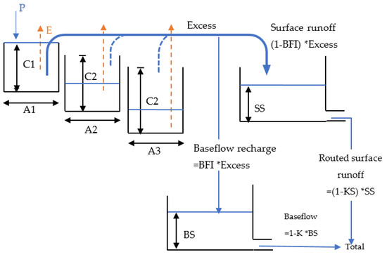
Figure 3. The AWMB description and structure to simulate runoff.

Because the evapotranspiration demand exceeds the available moisture, if the store’s moisture value reaches negative, it is reset to zero. If the amount of moisture in the store exceeds its capacity, the excess moisture becomes runoff, and the store is restored to its original capacity. Only $A1$ and $A2$ can be set because the three parameters $A1$, $A2$, and $A3$ reflecting the proportions of the catchment areas; $A3$ will be updated to respect the constraint if $A1$ and/or $A2$ are changed.

If there is base flow in the stream flow, part of the runoff from any store becomes recharged of the base flow store. $BFI$*runoff is the percentage of runoff utilized to replenish the base flow store, where $BFI$ is the base flow index, or the ratio of base flow to total flow in the stream flow. Surface runoff accounts for the balance of the runoff, i.e., (1.0 − BFI)*runoff. The base flow store depletes at a rate of $\left(1.0-K\right)\ast BS$, where $BS$ is the current moisture in the base flow store and $K$ is the time step’s base flow recession constant (daily or hourly).

To simulate the delay of surface runoff reaching the outlet of a medium–large catchment, the surface runoff can be routed through a store if necessary. The surface store depletes at the rate of $\left(1.0-KS\right)\ast SS$, where $SS$ is the current moisture in the surface runoff store and $KS$ is the surface runoff recession constant of the time step being used. All eight parameters range setup in the calibration, in shown in Table 2.

Table 2. Parameters of the AWBM and their ranges.

AWBM
Parameter	Range	Unit
$A1$	0–1	-
$A2$	0–1	-
$BFI$	0–1	-
$C1$	0–50	mm
$C2$	0–200	mm
$C3$	0–500	mm
$K_{Base}$	0–1	-
$K_{Surf}$	0–1	-

(b) 

Sacramento Soil Moisture Accounting (SAC-SMA) Model:

Burnash, et al. [55] developed the Sacramento model for the United States National Weather Service and the California Department of Water Resources. The model simulates the water balance within the watershed by using soil moisture accounting. Rainfall increases soil moisture storage, but evaporation and water movement out of the store lower it. The depth of rainfall absorbed, real evapotranspiration, and the amount of water moving vertically or laterally out of the storage are all determined by the size and relative wetness of the storage. Rainfall that is not absorbed generates runoff, which is converted using an empirical unit hydrograph or another technique. Streamflow is created by overlaying lateral water motions from soil moisture reserves on this runoff.

The Sacramento model uses a total of 16 parameters, as shown in Table 3, to depict the water balance, as follows:

Table 3. Parameters of SACRAMENTO model and their ranges.

SACRAMENTO Model
Parameter	Description	Range	Unit
LZPK	The ratio of water in LZFPM, which drains as base flow each day.	0.001–0.015	fraction
LZSK	The ratio of water in LZFSM, which drains as base flow each day.	0.03–0.2	fraction
UZK	The fraction of water in UZFWM, which drains as interflow each day.	0.2–0.5	fraction
UZTWM	Upper zone tension water maximum. The maximum volume of water held by the upper zone between field capacity and the wilting point which can be lost by direct evaporation and evapotranspiration from soil surface. This storage is filled before any water in the upper zone is transferred to other storages.	25–125	mm
UZFWM	Upper zone free water maximum: this storage is the source of water for interflow and the driving force for transferring water to deeper depths.	10–75	mm
LZTWM	Lower zone tension water maximum: the maximum capacity of lower zone tension water. Water from this store can only be removed through evapotranspiration.	75–300	mm
LZFSM	Lower zone free water supplemental maximum: the maximum volume from which supplemental base flow can be drawn.	15–300	mm
LZFPM	Lower zone free water primary maximum: the maximum capacity from which primary base flow can be drawn.	40–600	mm
PFREE	The minimum proportion of percolation from the upper zone to the lower zone directly available for recharging the lower zone free water stores.	0–0.5	percent/100
REXP	An exponent determining the rate of change of the percolation rate with changing lower zone water storage.	0–3	none
ZPERC	The proportional increase in Pbase that defines the maximum percolation rate.	0–80	none
SIDE	The ratio of non-channel baseflow (deep recharge) to channel (visible) baseflow.	0–0.8	ratio
SSOUT	The volume of the flow which can be conveyed by porous material in the bed of stream.	0–0.1	mm
PCTIM	The permanently impervious fraction of the basin contiguous with stream channels, which contributes to direct runoff.	0–0.05	percent/100
ADIMP	The additional fraction of the catchment, which develops impervious characteristics under soil saturation conditions.	0–0.2	percent/100
SARVA	A decimal fraction representing that portion of the basin normally covered by streams, lakes, and vegetation that can deplete stream flow by evapotranspiration.	0–0.1	percent/100
RSERV	Fraction of lower zone free water unavailable for transpiration.	0–0.4	percent/100
UH1	The first component of the unit hydrograph, i.e., the proportion of instantaneous runoff not lagged.	0–1	percent/100
UH2	The second component of the unit hydrograph, i.e., the proportion of instantaneous runoff runoff lagged by one time-step.	0–1	percent/100
UH3	The third component of the unit hydrograph, i.e., the proportion of instantaneous runoff runoff lagged by two time-steps.	0–1	percent/100
UH4	The fourth component of the unit hydrograph, i.e., the proportion of instantaneous runoff runoff lagged by three time-steps.	0–1	percent/100
UH5	The fifth component of the unit hydrograph, i.e., the proportion of instantaneous runoff runoff lagged by four time-steps.	0–1	percent/100

-

Five parameters define the soil moisture store (UZTWM, UZFWM, LZTWM, LZFSM, and LZFPM).

-

Three parameters calculate the rate of lateral outflow (LZPK, LZSK, and UZK).

-

Three parameters calculate the percolation water from the upper to the lower soil moisture stores (PFREE, REXP, and ZPERC).

-

Two parameters calculate direct runoff (PCTIM and ADIMP).

-

Three parameters calculate losses in the system (SIDE, SSOUT, and SARVA).

-

Five parameters allow time delays to be applied to instantaneous runoff (UH1–UH5).

-

RSERV, the final parameter, has a very low sensitivity; therefore, optimizing it is usually not necessary.

(c) 

The SIMHYD Model:

The SIMHYD model is a simplified version of HYDROLOG, a daily conceptual rainfall runoff model developed by Porter and McMahon [56], and MODHYDROLOG, a more contemporary model [57]. The SIMHYD model has 7 parameters, as shown in Table 4, as compared with the 17 parameters required for HYDROLOG and the 19 required for MODHYDROLOG.

Table 4. Parameters of the SIMHYD model and their ranges.

	SIMHYD
Parameter	Description	Range	Unit
Baseflow Coeff.	Base flow Coefficient	0–1	-
Impervious Threshold	Impervious Threshold	0–5	mm
Infiltration Coeff.	Infiltration Coefficient	0–400	-
Infiltration shape	Infiltration Shape	0–10	-
Interflow Coeff.	Interflow Coefficient	0–1	-
Perv. Fraction	Pervious Fraction	0–1	-
RISC	Rainfall Interception Store Capacity	0–5	mm
Recharge coefficient	Recharge Coefficient	0–1	-
SMSC	Soil Moisture Store Capacity	1–500	mm

Daily rainfall in SIMHYD first fills the interception store, which is then drained by evaporation each day. The excess rainfall is then run through an infiltration function to assess the capacity of infiltration. Excess rainfall that exceeds the capability of infiltration is known as infiltration excess runoff. Moisture that infiltrates is diverted to the stream (interflow), groundwater storage (recharge), and soil moisture store via a soil moisture function. The interflow is first calculated as a linear function of soil moisture (soil moisture level divided by soil moisture capacity). As a result, the equation employed to approximate interflow tries to replicate both interflow and saturation surplus runoff processes (with the soil wetness used to reflect parts of the catchment that are saturated, from which saturation excess runoff can occur). The recharge of groundwater is then calculated as a linear function of soil wetness. The remaining moisture is absorbed by the soil moisture storage system. The rate of areal potential evapotranspiration from the soil moisture store is estimated as a linear function of soil wetness, although it cannot exceed the atmospherically controlled rate. The capacity of the soil moisture store is limited, and it overflows into the groundwater store. The groundwater store’s base flow is modeled as a linear recession from the store. Infiltration excess runoff, interflow (and saturation excess runoff), and base flow are the three sources of runoff estimated by the model.

3. Application of the Daily Water Balance Model

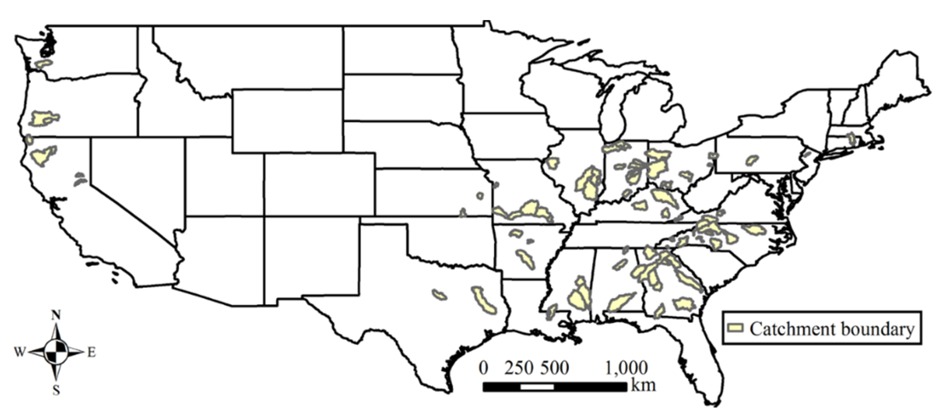
The developed PDM–CN model was applied to 92 catchments from the MOPEX (model parameter estimation experiment) dataset [58]. Figure 4 shows the spatial distribution of these study catchments with catchment areas ranging from 134 to 9886 km², presented in Table 5. The mean temperature of the catchments ranges from 9 to 21 °C, and the climate aridity index ranges from 0.27 to 1.91, and the runoff coefficient ranges from 0.09 to 0.80. These catchments were selected based on the criteria of minimum human interferences [59] and snow effect. The catchments with an average temperature less than −2 °C during the months from November to April were excluded to minimize the snow effect [60,61,62]. Daily precipitation, maximum and minimum air temperature, and streamflow observations were obtained from the MOPEX dataset. Daily potential evaporation data were estimated using the Priestley–Taylor method [63] at the spatial resolution of 8 by 8 km [64]. The daily precipitation and potential evaporation during 1948–2003 were the inputs for the daily water balance model, and the daily streamflow data was used for model calibration and validation.

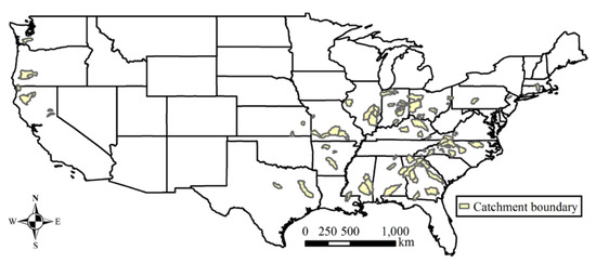
Figure 4. The location and boundary of the study catchments where the proposed daily water balance model is applied.

Table 5. Description of the 92 catchment areas located in the U.S.

Site ID	Area (km2)	Location	Longitude	Latitude	Ep/P	Ta (°C)
01127000	1847	QUINEBAUG R At JEWETT CITY, CT.	−71.985	41.598	0.603	10.162
01445500	275	PEQUEST RIVER at PEQUEST, NJ.	−74.979	40.831	0.630	10.750
01559000	2113	JUNIATA RIVER at HUNTINGDON, PA.	−78.019	40.485	0.807	10.907
02055000	1023	ROANOKE RIVER at ROANOKE, VA.	−79.939	37.258	0.786	13.367
02083500	5654	TAR RIVER at TARBORO, NC.	−77.533	35.894	0.862	16.929
02102000	3714	DEEP RIVER at MONCURE, NC.	−79.116	35.627	0.805	16.725
02116500	5905	YADKIN RIVER at YADKIN COLLEGE, NC.	−80.386	35.857	0.709	15.173
02118000	793	SOUTH YADKIN RIVER NEAR MOCKSVILLE, NC.	−80.659	35.845	0.734	15.805
02126000	3553	ROCKY RIVER NEAR NORWOOD, NC.	−80.176	35.148	0.821	17.360
02138500	173	LINVILLE RIVER NEAR NEBO, NC.	−81.890	35.795	0.562	12.557
02143000	215	HENRY FORK NEAR HENRY RIVER, NC.	−81.403	35.684	0.673	15.946
02143500	179	INDIAN CREEK NEAR LABORATORY, NC.	−81.264	35.422	0.752	16.845
02192000	3704	BROAD RIVER NEAR BELL, GA.	−82.770	33.974	0.803	17.417
02202500	6863	OGEECHEE RIVER NEAR EDEN, GA.	−81.416	32.191	0.919	19.372
02217500	1015	MIDDLE OCONEE RIVER NEAR ATHENS, GA.	−83.423	33.947	0.752	17.311
02228000	7226	SATILLA RIVER at ATKINSON, GA.	−81.868	31.221	0.919	20.628
02329000	2953	OCHLOCKONEE RIVER NR HAVANA, FL.	−84.384	30.554	0.829	21.036
02339500	9194	CHATTAHOOCHEE RIVER at WEST POINT, GA.	−85.182	32.886	0.691	17.120
02347500	4791	FLINT RIVER NEAR CULLODEN, GA.	−84.233	32.721	0.817	18.404
02349500	7511	FLINT RIVER at MONTEZUMA, GA.	−84.044	32.298	0.843	18.778
02375500	9886	ESCAMBIA RIVER NEAR CENTURY, FL.	−87.234	30.965	0.726	19.968
02387000	1779	CONASAUGA RIVER at TILTON, GA.	−84.928	34.667	0.613	16.251
02387500	4149	OOSTANAULA RIVER at RESACA, GA.	−84.941	34.578	0.596	16.208
02414500	4338	TALLAPOOSA RIVER at WADLEY, AL.	−85.561	33.117	0.708	17.111
02456500	2292	LOCUST FORK at SAYRE, AL.	−86.983	33.710	0.699	17.571
02472000	1924	LEAF RIVER NR COLLINS, MS.	−89.407	31.707	0.730	19.188
02143000	9052	LEAF RIVER NR MCLAIN, MS.	−88.808	31.103	0.722	19.523
02475500	956	CHUNKY RIVER NR CHUNKY, MS.	−88.910	32.326	0.743	18.692
02478500	6967	CHICKASAWHAY RIVER AT LEAKESVILLE, MS.	−88.548	31.148	0.727	19.211
02482000	2341	PEARL RIVER at EDINBURG, MS.	−89.335	32.798	0.755	18.506
03109500	1285	L BEAVER C NR EAST LIVERPOOL, OH.	−80.541	40.676	0.840	11.534
03111500	319	SHORT C NR DILLONVALE, OH.	−80.734	40.193	0.774	12.370
03159500	2442	HOCKING R at ATHENS, OH.	−82.088	39.329	0.845	12.557
03161000	531	SOUTH FORK NEW RIVER NEAR JEFFERSON, NC.	−81.407	36.393	0.569	12.163
03164000	2929	NEW RIVER NEAR GALAX, VA.	−80.979	36.647	0.638	12.155
03168000	5703	NEW RIVER AT ALLISONIA, VA.	−80.746	36.937	0.694	12.411
03237500	1002	OHIO BRUSH C NR WEST UNION, OH.	−83.421	38.804	0.793	13.567
03238500	565	WHITEOAK C NR GEORGETOWN, OH.	−83.929	38.858	0.781	13.014
03253500	8547	LICKING RIVER at CATAWBA, KY.	−84.311	38.710	0.726	14.229
03265000	1303	STILLWATER R at PLEASANT HILL, OH.	−84.356	40.058	0.924	11.881
03266000	1683	STILLWATER R at ENGLEWOOD, OH.	−84.283	39.869	0.919	12.072
03269500	1269	MAD R NR SPRINGFIELD, OH.	−83.870	39.923	0.896	11.905
03274000	9402	G MIAMI R at HAMILTON, OH.	−84.572	39.391	0.894	12.302
03281500	1870	SOUTH FORK KENTUCKY RIVER at BOONEVILLE, KY.	−83.677	37.479	0.648	14.666
03301500	3364	ROLLING FORK NR BOSTON, KY.	−85.704	37.767	0.719	14.859
03303000	1233	BLUE RIVER NEAR WHITE CLOUD, IND	−86.228	38.237	0.779	14.296
03326500	1766	MISSISSINEWA RIVER at MARION, IND.	−85.659	40.576	0.894	11.977
03339500	1318	SUGAR CREEK at CRAWFORDSVILLE, IND.	−86.899	40.049	0.882	12.555
03345500	3926	EMBARRAS RIVER at STE. MARIE, IL.	−88.019	38.936	0.952	13.173
03346000	824	NORTH FORK EMBARRAS RIVER NEAR OBLONG, IL.	−87.946	39.010	0.927	13.419
03349000	2222	WHITE RIVER at NOBLESVILLE, IN.	−86.017	40.047	0.879	12.148
03361500	1090	BIG BLUE RIVER at SHELBYVILLE, IN.	−85.782	39.529	0.827	12.449
03362500	1228	SUGAR CREEK NEAR EDINBURGH, IN.	−85.998	39.361	0.820	12.631
03364000	4421	EAST FORK WHITE RIVER at COLUMBUS, IND.	−85.926	39.200	0.829	12.699
03365500	6063	EAST FORK WHITE RIVER at SEYMOUR, IND.	−85.899	38.983	0.821	12.849
03381500	8034	LITTLE WABASH RIVER at CARMI, IL.	−88.160	38.061	0.964	14.006
03443000	767	FRENCH BROAD RIVER at BLANTYRE, NC.	−82.624	35.299	0.432	13.878
03451500	2448	FRENCH BROAD RIVER at ASHEVILLE, NC.	−82.579	35.609	0.543	13.989
03504000	134	NANTAHALA RIVER NEAR RAINBOW SPRINGS, NC.	−83.619	35.127	0.389	12.819
03512000	477	OCONALUFTEE RIVER at BIRDTOWN, NC.	−83.354	35.461	0.428	12.284
03531500	826	POWELL RIVER NEAR JONESVILLE, VA.	−83.095	36.662	0.595	13.949
03574500	829	PAINT ROCK RIVER NEAR WOODVILLE, AL.	−86.306	34.624	0.622	16.334
04191500	6004	AUGLAIZE R NR DEFIANCE, OH.	−84.399	41.238	0.977	11.793
05515500	1391	KANKAKEE RIVER at DAVIS, IND.	−86.701	41.400	0.907	11.081
05520500	5941	KANKAKEE RIVER at MOMENCE, IL.	−87.669	41.160	0.929	11.199
05584500	1696	LA MOINE RIVER at COLMAR, IL.	−90.899	40.329	1.076	12.239
05585000	3349	LA MOINE RIVER at RIPLEY, IL.	−90.632	40.025	1.073	12.372
05592500	5025	KASKASKIA RIVER at VANDALIA, IL.	−89.089	38.960	0.994	13.066
05593000	7042	KASKASKIA RIVER at CARLYLE, IL.	−89.356	38.612	1.013	13.251
06894000	477	LITTLE BLUE RIVER NEAR LAKE CITY, MO.	−94.300	39.101	1.130	13.883
06914000	865	POTTAWATOMIE C NR GARNETT, KS.	−95.249	38.334	1.256	13.869
06933500	7356	GASCONADE RIVER at JEROME MO.	−91.977	37.930	0.925	13.821
07052500	2556	JAMES RIVER at GALENA, MO.	−93.461	36.805	0.943	13.996
07056000	2147	BUFFALO RIVER NEAR ST. JOE, ARK.	−92.746	35.984	0.784	14.355
07067000	4318	CURRENT RIVER at VAN BUREN, MO.	−91.015	36.991	0.881	14.058
07068000	5278	CURRENT RIVER at DONIPHAN, MO.	−90.848	36.622	0.870	14.257
07172000	1153	CANEY R NR ELGIN, KS.	−96.315	37.004	1.448	14.563
07186000	3015	SPRING RIVER NEAR WACO, MO.	−94.566	37.246	1.014	14.462
07261000	438	CADRON CREEK NEAR GUY, ARK.	−92.403	35.299	0.753	15.811
07363500	5444	SALINE RIVER NEAR RYE, ARK.	−92.026	33.701	0.720	17.515
07378000	736	COMITE RIVER NEAR COMITE, LA.	−91.074	30.512	0.697	20.264
07378500	3315	AMITE RIVER NEAR DENHAM SPRINGS, LA.	−90.990	30.464	0.682	20.090
08033500	9417	NECHES RIVER NEAR ROCKLAND, TEX.	−94.399	31.025	1.139	19.792
08095000	2507	NORTH BOSQUE RIVER NR CLIFTON, TX.	−97.568	31.786	1.915	18.968
11342000	1101	SACRAMENTO R A DELTA CA.	−122.416	40.940	0.579	10.273
11413000	647	N YUBA R BL GOODYEARS BAR CA.	−120.937	39.525	0.690	9.286
11427000	886	NF AMERICAN R A NORTH FORK DAM CA.	−121.023	38.936	0.777	10.188
11530000	7389	TRINITY R A HOOPA CA.	−123.671	41.050	0.721	11.062
11532500	1589	SMITH R NR CRESCENT CITY CA.	−124.054	41.789	0.272	10.525
12027500	2318	CHEHALIS RIVER NEAR GRAND MOUND, WASH.	−123.034	46.776	0.379	9.988
14308000	1163	S. UMPQUA RIVER TILLER, OR.	−122.947	42.931	0.622	9.225
14321000	9539	UMPQUA RIVER NEAR ELKTON, OREG.	−123.554	43.586	0.598	10.210

T_a is the average temperature in °C; Ep/P is the aridity index.

The available data during 1948–2003 is divided into three periods, as follows: (1) the warm-up period during 1948–1953; (2) the calibration period during 1954–1973; (3) the validation period during 1974–2003. During the calibration period, the model parameters were estimated using the genetic algorithm (GA), which has been used for parameter estimation of hydrologic models [65]. There are five parameters for calibration: $a$ and $S_b$ are parameters for describing the spatial distribution of soil water storage capacity; $\gamma$ is used for the partitioning of runoff into direct runoff and groundwater recharge; $k_d$ and $k_b$ are parameters for routings of quick flow and base flow. The ranges of the five parameters for calibration are shown in Table 1. The objective function of calibration is to maximize the Nash and Sutcliffe efficiency (NSE) (Nash and Sutcliffe, 1970), as follows:

$$NSE=1-\frac{{{\displaystyle \sum }}_{t=1}^T{\left(Q_m^t–Q_o^t\right)}^2}{{{\displaystyle \sum }}_{t=1}^T{\left(Q_o^t-\overline{Q_o} \right)}^2}$$

(15)

where $Q_o^t$ is the observed daily streamflow at time $t$; $Q_m^t$ is simulated daily streamflow; $\overline{Q_o}$ is the mean observed streamflow; and $T$ is the total number of days for calibration. The NSE in Equation (15) has been used as an objective function in many studies [66,67,68].

4. Results and Discussion

The results for the application of the proposed PDM–CN model to the 92 catchments are presented in this section.

4.1. Model Performance

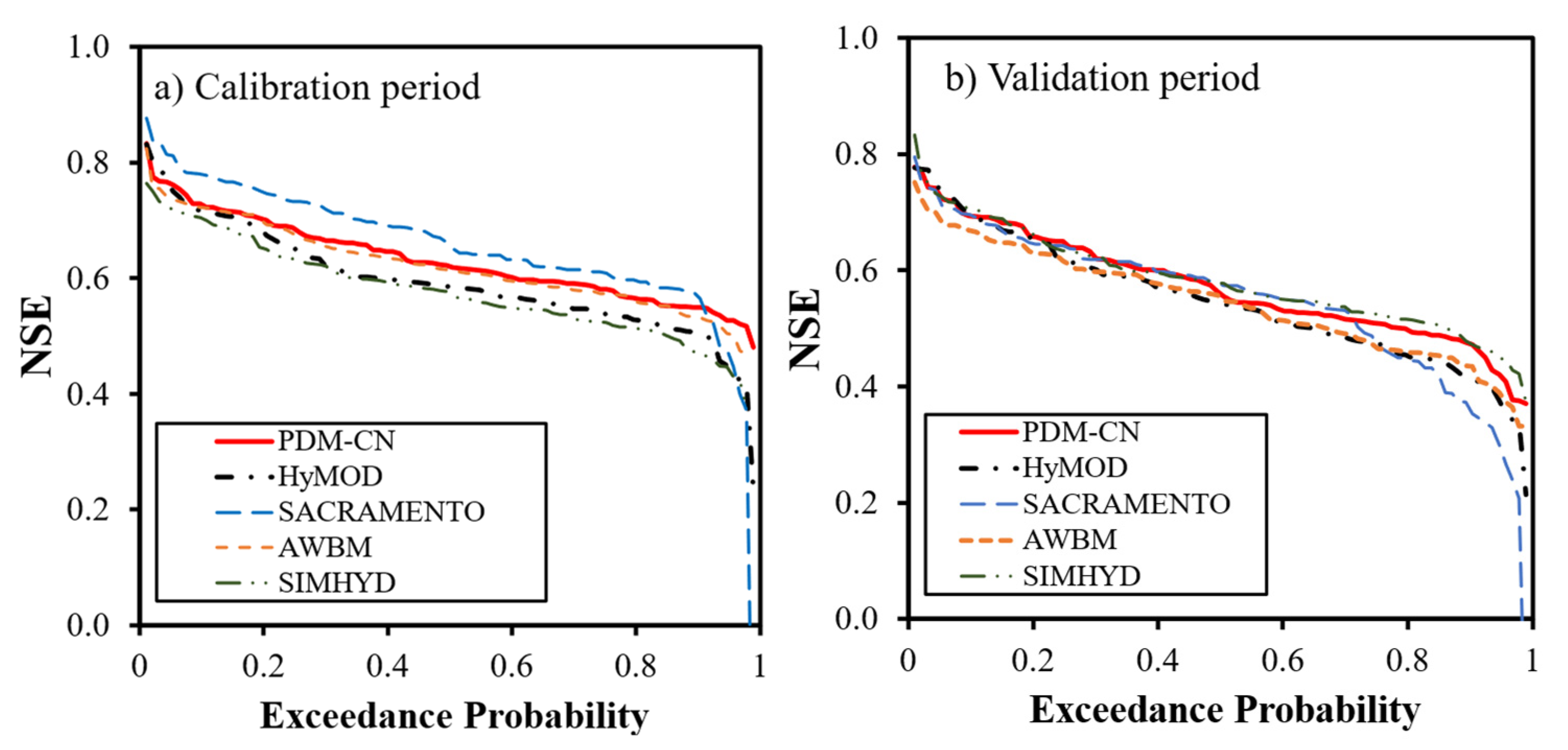
The NSE values during the calibration and validation periods were computed to evaluate the performance of the model. During the validation period, 8 catchments had an NSE value greater than 0.7; 30 catchments had an NSE value between 0.7 and 0.6; 36 catchments had an NSE value between 0.6 and 0.5. Figure 5 compares the NSE values between the proposed PDM–CN model, HyMOD, AWMB, SACRAMENTO, and SIMHYD models. In Table 6, the NSE values are categorized to explicitly show the performance in each category, from strong (1–0.75), to moderate (0.67–0.75), and ending with very weak (<0.59), which shows a better performance for PDM–CN over HyMOD in both strong and moderate NSE categories. In the strong calibrated NSE category, the HyMOD showed strong calibration in 5 catchments, while showing in 6 catchments in the unified model. Additionally, in the moderate category, the unified model showed 20 catchments, versus 15 from the HyMOD model in the calibration period. The calibration results show NSE values for each row, for specific calibration–validation combinations, suggesting that the calibration results are somewhat better than the validation results, as expected [69].

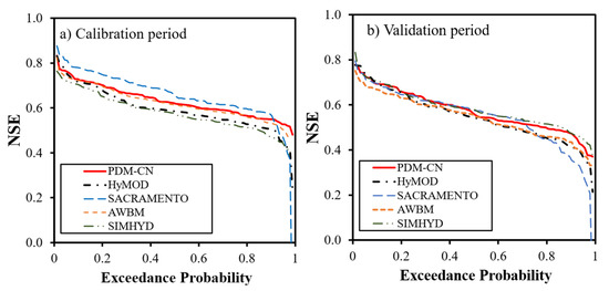
Figure 5. The exceedance probability of the number of catchments, with respect to NSE, during the calibration (a) and validation (b) periods.

Table 6. Categories of Nash–Sutcliffe efficiency (NSE) for catchments in calibration and validation periods.

	Calibration Period					Validation Period
NSE (Catchments)	HyMOD	PDM–CN	AWBM	SAC *	SIMHYD	HyMOD	PDM–CN	AWBM	SAC *	SIMHYD
Strong (1–0.75)	5	6	3	18	2	3	2	1	2	1
Moderate (0.67–0.75)	15	20	20	27	16	10	15	7	11	5
Weak (0.59–0.67)	26	39	37	31	20	18	23	26	29	15
Very weak (<0.59)	46	27	32	16	54	61	52	58	50	70

* SAC is an abbreviation for the SCARAMENO model.

Figure 5a shows the percentage of catchments with NSE value greater than a certain value during the calibration period. For example, 40% of catchments have an NSE value greater than 0.65 for the proposed PDM–CN model and 0.60 for the HyMOD. Figure 5b shows the corresponding comparison during the validation period, and 40% of catchments have an NSE value greater than 0.60 for the PDM–CN model and 0.57 for the HyMOD model. As shown in Figure 5, the performance of the proposed PDM–CN model is slightly better than the HyMOD, AWMB, and SIMHYD models but it could not overcome the performance of the SACRAMENTO model during the calibration period. However, the PDM–CN model is nearly better than or equal to over 50% of the NSE values in the validation period compared to the SACRAMENTO model, which has 16 parameters, the AWMB model with 8 parameters, and the SIMHYD model with 7 parameters. As discussed earlier, the main differences between these models and the PDM–CN are the following: (1) different distribution functions used for describing soil water storage capacity; (2) computation of evaporation. In the remainder of the paper, the simulation results for the proposed model are presented. The structure of the PDM–CN parameters in Equation (3), which represents the soil wetting ($W$), and the runoff in Equation (8). Wetter soil creates more surface runoff in drier soil ($m$ = 0), given the same amount of precipitation and storage capacity, and the difference is higher for watersheds with larger average storage capacity. For watersheds with larger average storage capacity, the shape parameter, $a$, in Equation (1) has a considerable impact on runoff generation. Additionally, in the PDM–CN model, the initial abstraction is dependent on the shape parameter, $a$, which is not the same as the SCS–CN initial abstraction, which is based on average storage capacity. As for the AWBM and SimHyd, the model structure comparison by Yu and Zhu [69] summarized that parameterization varies; these conceptual models are essentially ways of speaking to the nonlinear relationship between the compelling precipitation and runoff sum. The AWBM and the SimHyd model were developed in Australia; therefore, a limitation to accurately reproduce runoff in snowy areas was not considered similar to the SACRAMENTO and PDM–CN models. Nevertheless, the models’ performance using the genetic algorithm was successful in calibration. However, various parameters, including population size, crossover probability, mutation probability, and halting criterion, can all affect the effectiveness of the genetic algorithm. The effect of various combinations of these on the algorithm should be investigated [70].

4.2. Soil Water Storage Capacity

The distribution function for soil water storage capacity is the most important component for the PDM–CN model since it determines the partitioning between runoff and soil wetting and the calculation of evaporation. Figure 6a shows the frequency distribution of the estimated shape parameter for the distribution function, shown in Equation (1).

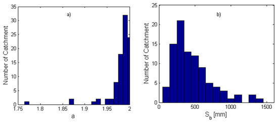
Figure 6. The frequency distribution of the calibrated parameters for the distribution function for soil water storage capacity: (a) the shape parameter (a); (b) the mean of the distribution $\left(S_b\right)$.

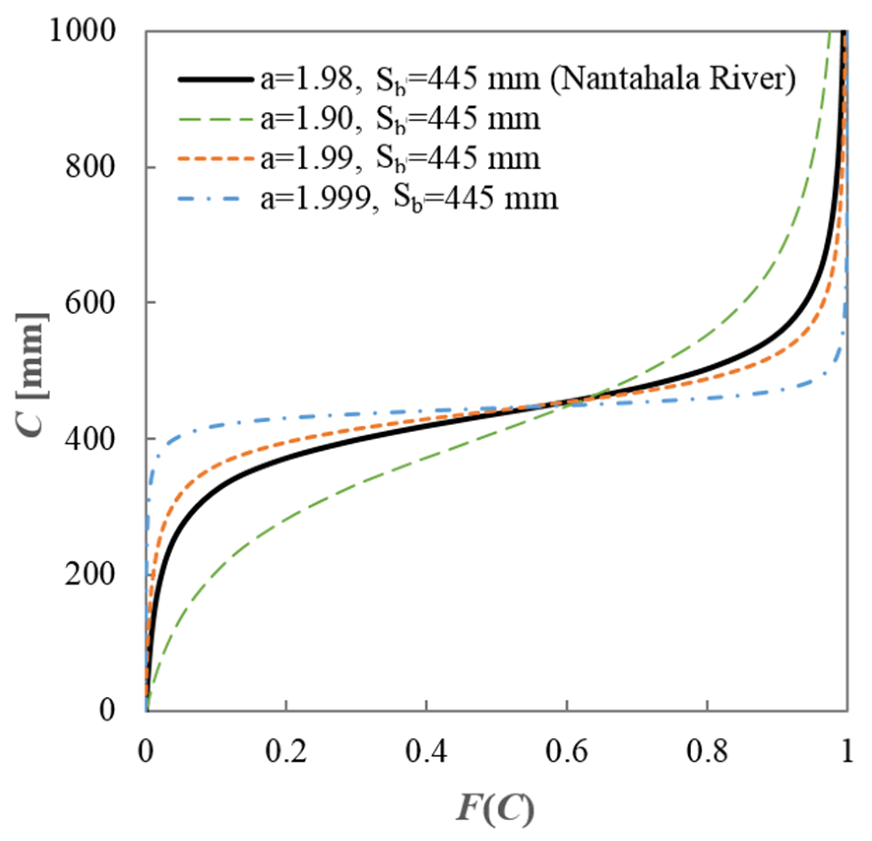
As shown in Table 1, the range for the shape parameter (a) is set to [0.01, 2.0]. However, the estimated parameters for all the catchments are greater than 1.75. That indicates that the CDF of the distributions is S-shaped [52]. For example, Figure 7 plots the CDF of the soil water storage capacity for the Nantahala River, located in North Carolina.

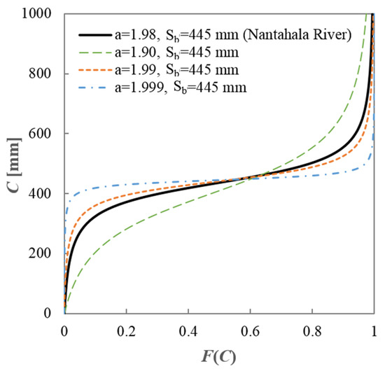
Figure 7. The estimated cumulative distribution of soil water storage capacity in the Nantahala River, North Carolina (USGS gage #03504000), and sensitivities of the shape parameter (a).

The catchment is located in a humid area with a climate aridity index of 0.39. The USGS streamflow gage number is 03504000 with a drainage area of 134 km². The estimated shape parameter (a) is 1.98 and the mean of the distribution ($S_b$) is 445 mm. Particularly, the shape parameter of most catchments is between 1.90 and 2.0. To show the sensitivity of CDF to the shape parameter, Figure 7 plots the CDF for other 3 shape parameters, i.e., 1.90, 1.99, and 1.999 for the same value of $S_b$. As we can see, CDF is quite sensitive to $a$ from 1.9 to 2.0. With the increase in $a$, the soil water storage capacity becomes more uniformly distributed in space. Figure 6b shows the frequency distribution of the estimated mean value for the distribution function shown in Equation (1). As shown in Table 1, the range for $S_b$ is set to [50, 1500]. The mean storage capacity for most catchments (86 out of 92) are less than 1000 mm. The peak of the frequency distribution is at 200~300 mm. The majority of the catchments are within the range of 200~600 mm. As shown in Figure 7, the estimated $S_b$ for Nantahala River is 445 mm.

4.3. Simulated Streamflow and Evaporation

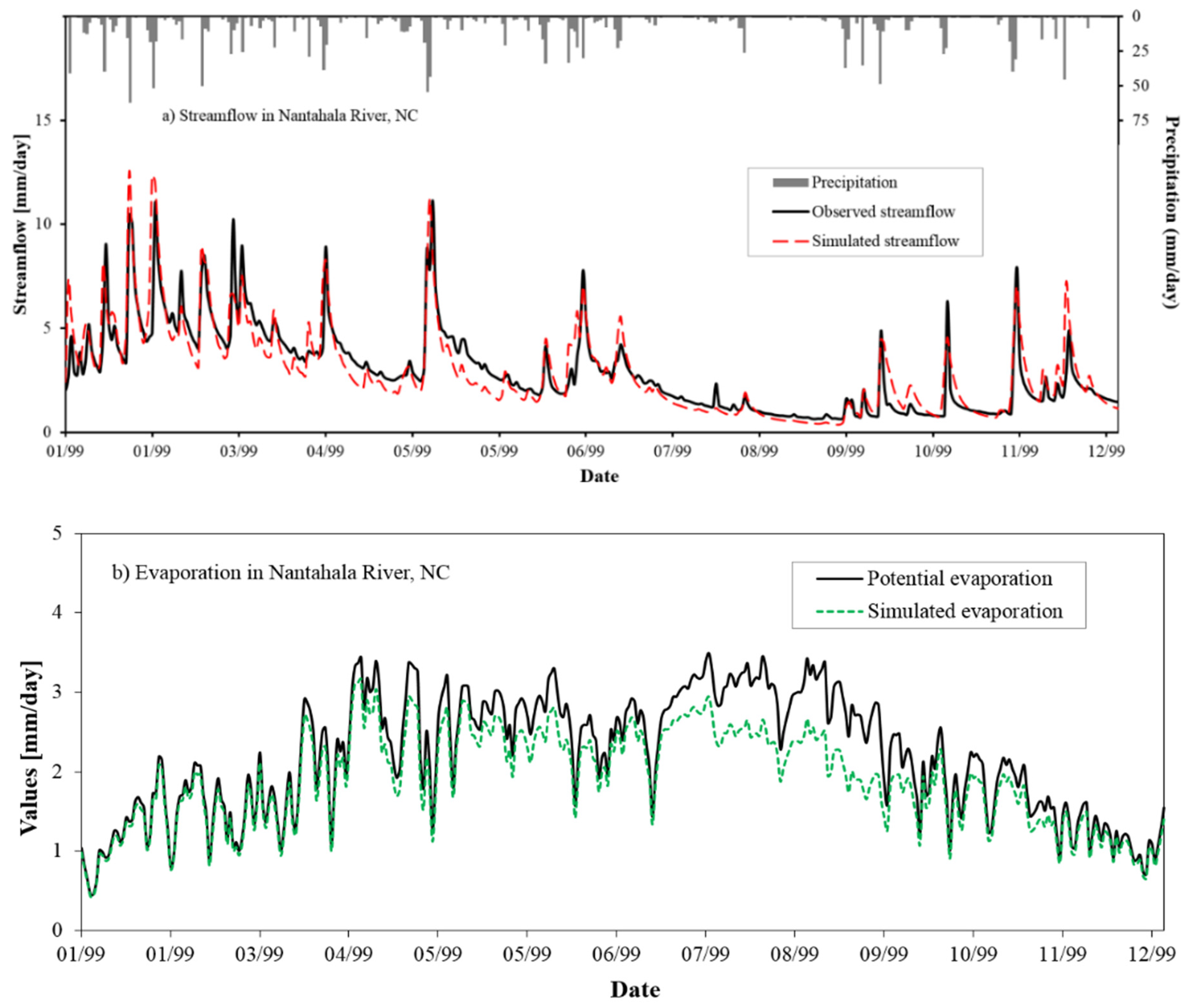
For demonstration purposes, the simulated streamflow and evaporation for the Nantahala River catchment are presented in Figure 8. The estimated parameters for the catchments are $a$ = 1.98, $S_b$ = 445 mm, $\gamma$ = 0.46, $k_d$ = 0.31 day⁻¹, and $k_b$ = 0.03 day⁻¹. The NSE value is 0.78 during the calibration period and 0.74 during the validation period. Figure 8a compares the observed and simulated daily streamflow for one year (i.e., 1999) in this catchment.

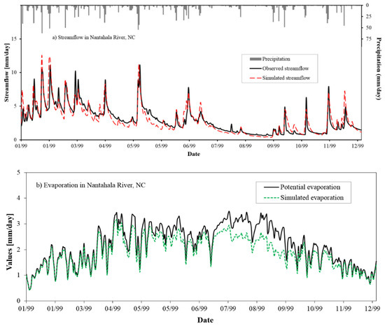
Figure 8. Simulation results for the Nantahala River, North Carolina (USGS gage #03504000), during the calendar year of 1999: (a) daily streamflow; (b) evaporation.

Figure 8b compares the potential evaporation to the simulated evaporation, which shows that simulated evaporation does not exceed potential evaporation. Therefore, during the summer, the temperature is too high, and the air is too dry. As a result, the rate of evaporation increases [71,72].

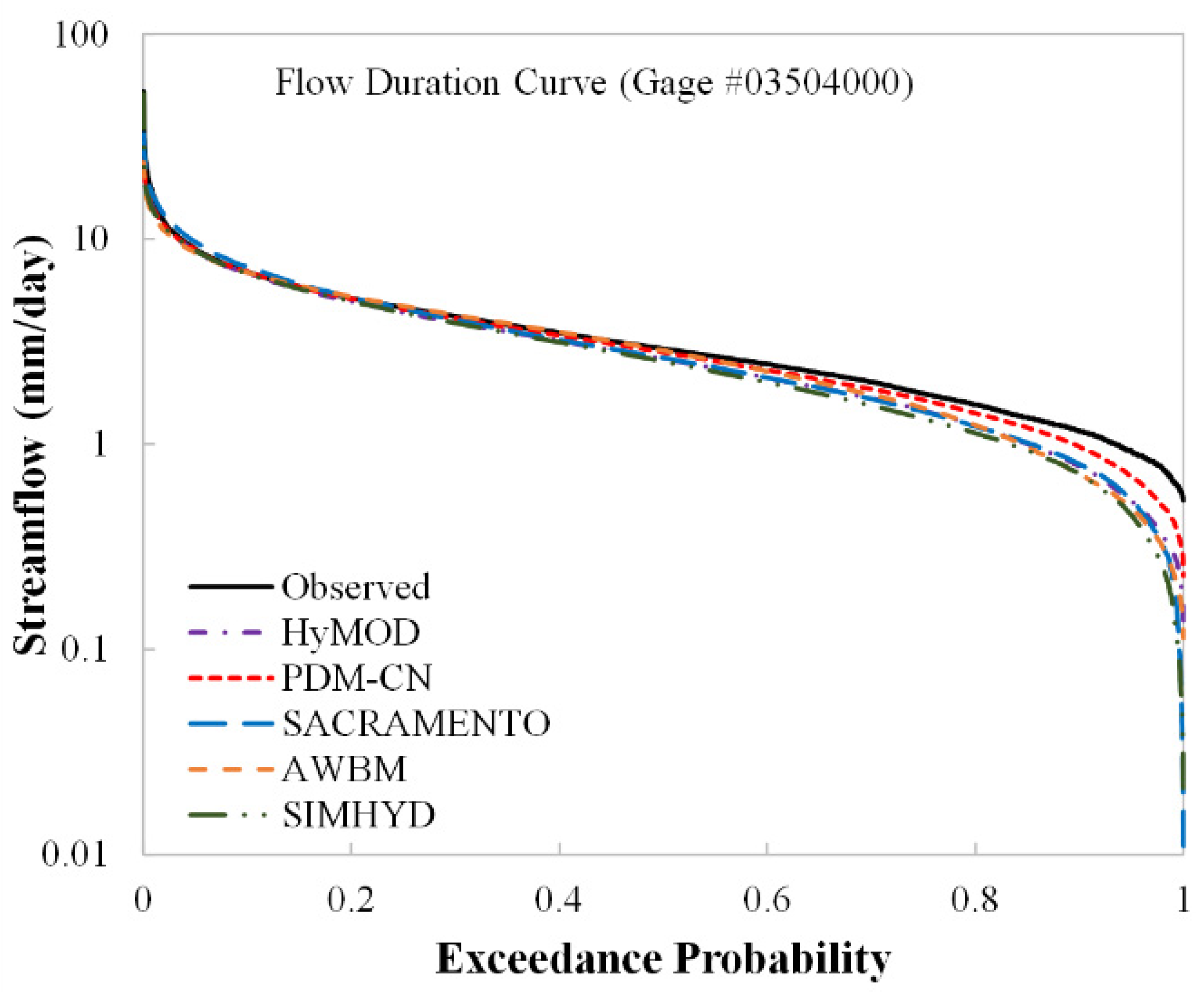
Figure 9 compares the observed and simulated (PDM–CN model) flow duration curves (FDC) during the validation period. The lower part of the unified model (PDM–CN) FDC is slightly lower than the observed one and goes further, lower, than other compared models (HyMOD, SACRAMENTO, AWBM, and SIMHYD); however, the simulated FDC matches the observed one well in other parts. Figure 8b shows the daily potential evaporation and simulated daily evaporation, which is computed by Equation (8), considering the spatial variability of soil water storage. In summary, conceptual models are most commonly viewed and recognized as useful tools for simulating observed streamflow. While model parameters are ostensibly physical, they are mostly utilized to characterize this nonlinear relationship. The considerable range in the calibrated parameter values over time may support the notion of equifinality [73], but it also suggests that assigning physical meanings to parameter values is likely fruitless. For the Nantahala River watershed, the PDM–CN model performed somewhat better than the HyMOD, SACRAMENTO, AWBM, and SIMHYD models.

Figure 9. Observed and simulated flow duration curves during the validation period (1974–2003) for the Nantahala River in North Carolina.

4.4. Linkage to Budyko Equation

If Equations (3) and (7) are applied to the mean annual water balance directly, $P$ and $E_P$ are the mean annual precipitation and the mean annual potential evaporation, respectively. For the mean annual water balance, the impact of initial water storage is negligible. Therefore, $S_0$ is set to 0, as it is in the SCS–CN method. Substituting $W$ from Equation (3) into Equation (7), the following equation is obtained:

$$\frac{E}{P}=\frac{1+{\phi }^{-1}-\sqrt{{\left(1+{\phi }^{-1}\right)}^2-2a{\phi }^{-1}}}{a^2}\left[\frac{E_P}{P}+\phi -\sqrt{{\left(\frac{E_P}{P}+\phi \right)}^2-2a\phi \frac{E_P}{P}}\right]$$

(16)

where,

$$\phi =\frac{S_b}{P}$$

(17)

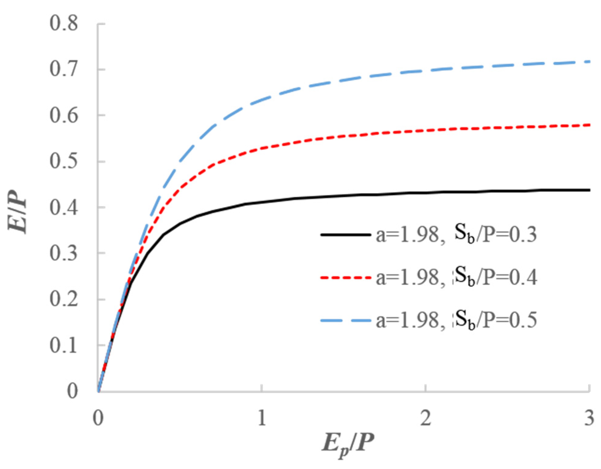
Equation (16) shows that the long-term evaporation ratio, i.e., $\frac{E}{P}$, can be written as a function of climate aridity index, $\left(\frac{E_P}{P}\right)$, the ratio of soil water storage capacity and mean annual precipitation ($\phi$), and the shape parameter of the distribution of soil water storage capacity ($a$).

For example, Figure 10 plots Equation (16) for three values of $\frac{S_b}{P}$ with a = 1.98. The evaporation ratio increases with $\frac{S_b}{P}$ for a given climate aridity index. Equation (16) captures control of $\frac{E_P}{P}$ and $\frac{S_b}{P}$ (i.e., climate and soil water storage capacity) on a long-term water balance. This equation can be interpreted as a two-parameter Budyko equation, compared with the one-parameter Budyko equation developed by [74].

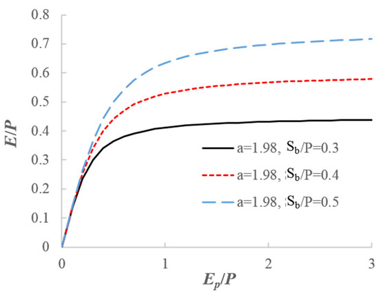
Figure 10. The obtained two-parameter, long-term water balance equation from the developed PDM–CN model.

5. Conclusions

In this paper, a new daily water balance model is developed, based on the new distribution function proposed by [52] for describing the spatial variability of soil water storage capacity. For a runoff generation perspective, the model is a PDM model, alike to the HyMOD model. When the initial soil water storage is neglected, this model becomes the SCS–CN method. Therefore, the model is a unified version of the HyMOD model and the SCS–CN method. Besides the distribution function for storage capacity, the calculation of evaporation in the model is also different from that of the HyMOD. In the developed PDM–CN model, the distribution function is also used for the calculation of evaporation, since the spatial variability of soil water storage also affects the catchment-scale evaporation. When applied to the long-term scale directly, the model leads to a two-parameter Budyko equation for a long-term water balance. Therefore, this model provides a unification for the PDM, the SCS–CN, and the Budyko models.

The developed 5-parameter model was applied to 92 catchments where the snow effect is minimal. The performance of the daily model was good in most catchments and was better than the HyMOD model, which is the currently used five-parameter daily water balance model; however, the performance was not entirely better when it was compared with the SCARAMENTO model, with 17 parameters in the calibration and validation periods, or when it was compared with the SIMHYD, with 7 parameters, in the period. Therefore, the PDM–CN model showed good results when it was compared with more sophisticated models, that have more than five parameters, such as the SACRAMENTO model, the SIMHYD model, and the AWBM. From the validation of the NSE results, 8 catchments had an NSE value greater than 0.7; 30 catchments had an NSE value between 0.7 and 0.6; 36 catchments had an NSE value between 0.6 and 0.5. Future research will explore the linkage between the estimated parameters ($a$ and $S_b$) and the curve number, considering the connection of this model with the SCS–CN method. The simplified version of the model will be applied for modeling monthly and annual water balance. For example, by removing the quick flow storage tank, the daily water balance model becomes a monthly water balance model; furthermore, by removing the slow flow storage tank, the monthly water balance model becomes an annual water balance model; in addition, through further removal of the soil water storage carryover, the annual water balance model becomes a mean annual water balance model (i.e., Equation (16)).

References

- Parra, V.; Fuentes-Aguilera, P.; Muñoz, E. Identifying advantages and drawbacks of two hydrological models based on a sensitivity analysis: A study in two Chilean watersheds. Hydrol. Sci. J. 2018, 63, 1831–1843. [Google Scholar] [CrossRef]
- Nicolle, P.; Pushpalatha, R.; Perrin, C.; François, D.; Thiéry, D.; Mathevet, T.; Le Lay, M.; Besson, F.; Soubeyroux, J.M.; Viel, C.; et al. Benchmarking hydrological models for low-flow simulation and forecasting on French catchments. Hydrol. Earth Syst. Sci. 2014, 18, 2829–2857. [Google Scholar] [CrossRef] [Green Version]
- Staudinger, M.; Stahl, K.; Seibert, J.; Clark, M.P.; Tallaksen, L.M. Comparison of hydrological model structures based on recession and low flow simulations. Hydrol. Earth Syst. Sci. 2011, 15, 3447–3459. [Google Scholar] [CrossRef] [Green Version]
- Li, B.; Rodell, M.; Sheffield, J.; Wood, E.; Sutanudjaja, E. Long-term, non-anthropogenic groundwater storage changes simulated by three global-scale hydrological models. Sci. Rep. 2019, 9, 10746. [Google Scholar] [CrossRef] [PubMed] [Green Version]
- Poelmans, L.; Van Rompaey, A.; Batelaan, O. Coupling urban expansion models and hydrological models: How important are spatial patterns? Land Use Policy 2010, 27, 965–975. [Google Scholar] [CrossRef]
- Beven, K.J.; Alcock, R.E. Modelling everything everywhere: A new approach to decision-making for water management under uncertainty. Freshw. Biol. 2012, 57, 124–132. [Google Scholar] [CrossRef] [Green Version]
- Lu, Z.; Wei, Y.; Feng, Q.; Western, A.W.; Zhou, S. A framework for incorporating social processes in hydrological models. Curr. Opin. Environ. Sustain. 2018, 33, 42–50. [Google Scholar] [CrossRef]
- Chung, E.-S.; Lee, K.S. Prioritization of water management for sustainability using hydrologic simulation model and multicriteria decision making techniques. J. Environ. Manag. 2009, 90, 1502–1511. [Google Scholar] [CrossRef]
- Ibrahim, B.; Wisser, D.; Barry, B.; Fowe, T.; Aduna, A. Hydrological predictions for small ungauged watersheds in the Sudanian zone of the Volta basin in West Africa. J. Hydrol. Reg. Stud. 2015, 4, 386–397. [Google Scholar] [CrossRef] [Green Version]
- Srinivasan, R.; Zhang, X.; Arnold, J. SWAT ungauged: Hydrological budget and crop yield predictions in the Upper Mississippi River Basin. Trans. ASABE 2010, 53, 1533–1546. [Google Scholar] [CrossRef]
- Sisay, E.; Halefom, A.; Khare, D.; Singh, L.; Worku, T. Hydrological modelling of ungauged urban watershed using SWAT model. Modeling Earth Syst. Environ. 2017, 3, 693–702. [Google Scholar] [CrossRef]
- Wagener, T.; Sivapalan, M.; McDonnell, J.; Hooper, R.; Lakshmi, V.; Liang, X.; Kumar, P. Predictions in ungauged basins as a catalyst for multidisciplinary hydrology. Eos Trans. Am. Geophys. Union 2004, 85, 451–457. [Google Scholar] [CrossRef] [Green Version]
- Kapangaziwiri, E.; Hughes, D.; Wagener, T. Incorporating uncertainty in hydrological predictions for gauged and ungauged basins in southern Africa. Hydrol. Sci. J. 2012, 57, 1000–1019. [Google Scholar] [CrossRef] [Green Version]
- Lin, Y.-P.; Hong, N.-M.; Wu, P.-J.; Wu, C.-F.; Verburg, P.H. Impacts of land use change scenarios on hydrology and land use patterns in the Wu-Tu watershed in Northern Taiwan. Landsc. Urban Plan. 2007, 80, 111–126. [Google Scholar] [CrossRef]
- Schilling, K.E.; Jha, M.K.; Zhang, Y.K.; Gassman, P.W.; Wolter, C.F. Impact of land use and land cover change on the water balance of a large agricultural watershed: Historical effects and future directions. Water Resour. Res. 2008, 44, 233. [Google Scholar] [CrossRef]
- Getachew, H.E.; Melesse, A.M. The impact of land use change on the hydrology of the Angereb Watershed, Ethiopia. Int. J. Water Sci. 2012, 1, 6. [Google Scholar]
- Paul, M.; Rajib, M.A.; Ahiablame, L. Spatial and temporal evaluation of hydrological response to climate and land use change in three South Dakota watersheds. JAWRA J. Am. Water Resour. Assoc. 2017, 53, 69–88. [Google Scholar] [CrossRef]
- Jiang, T.; Chen, Y.D.; Xu, C.-Y.; Chen, X.; Chen, X.; Singh, V.P. Comparison of hydrological impacts of climate change simulated by six hydrological models in the Dongjiang Basin, South China. J. Hydrol. 2007, 336, 316–333. [Google Scholar] [CrossRef]
- Devia, G.K.; Ganasri, B.P.; Dwarakish, G.S. A review on hydrological models. Aquat. Procedia 2015, 4, 1001–1007. [Google Scholar] [CrossRef]
- Krysanova, V.; Donnelly, C.; Gelfan, A.; Gerten, D.; Arheimer, B.; Hattermann, F.; Kundzewicz, Z.W. How the performance of hydrological models relates to credibility of projections under climate change. Hydrol. Sci. J. 2018, 63, 696–720. [Google Scholar] [CrossRef]
- Jones, R.N.; Chiew, F.H.; Boughton, W.C.; Zhang, L. Estimating the sensitivity of mean annual runoff to climate change using selected hydrological models. Adv. Water Resour. 2006, 29, 1419–1429. [Google Scholar] [CrossRef] [Green Version]
- Schaake, J.C.; Koren, V.I.; Duan, Q.Y.; Mitchell, K.; Chen, F. Simple water balance model for estimating runoff at different spatial and temporal scales. J. Geophys. Res. Atmos. 1996, 101, 7461–7475. [Google Scholar] [CrossRef]
- Burnash, R.; Ferral, R.; McQuire, R. A Generalized Streamflow Simulation System; Report; Joint Federal-State River Forecast Center: Sacramento, CA, USA, 1973. [Google Scholar]
- Zhang, L.; Potter, N.; Hickel, K.; Zhang, Y.; Shao, Q. Water balance modeling over variable time scales based on the Budyko framework–Model development and testing. J. Hydrol. 2008, 360, 117–131. [Google Scholar] [CrossRef]
- Budyko, M. Climate and Life; International Geophysical Series; Elsevier: Amsterdam, The Netherlands, 1974; Volume 18. [Google Scholar]
- Boyle, D.P.; Gupta, H.V.; Sorooshian, S. Multicriteria calibration of hydrologic models, in Calibration of Watershed Models. Water Sci. Appl. 2003, 6, 185–196. [Google Scholar] [CrossRef] [Green Version]
- Moore, R. The probability-distributed principle and runoff production at point and basin scales. Hydrol. Sci. J. 1985, 30, 273–297. [Google Scholar] [CrossRef] [Green Version]
- Kollat, J.; Reed, P.; Wagener, T. When are multiobjective calibration trade-offs in hydrologic models meaningful? Water Resour. Res. 2012, 48, 95. [Google Scholar] [CrossRef]
- Vrugt, J.A.; Gupta, H.V.; Bastidas, L.A.; Bouten, W.; Sorooshian, S. Effective and efficient algorithm for multiobjective optimization of hydrologic models. Water Resour. Res. 2003, 39, 373. [Google Scholar] [CrossRef] [Green Version]
- Wagener, T.; Boyle, D.P.; Lees, M.J.; Wheater, H.S.; Gupta, H.V.; Sorooshian, S. A framework for development and application of hydrological models. Hydrol. Earth Syst. Sci. 2001, 5, 13–26. [Google Scholar] [CrossRef]
- Wang, D.; Chen, Y.; Cai, X. State and parameter estimation of hydrologic models using the constrained ensemble Kalman filter. Water Resour. Res. 2009, 45, W11416. [Google Scholar] [CrossRef] [Green Version]
- Moore, R. The PDM rainfall-runoff model. Hydrol. Earth Syst. Sci. Discuss. 2007, 11, 483–499. [Google Scholar] [CrossRef]
- Zhao, R. Flood forecasting method for humid regions of China. East China Coll. Hydraul. Eng. Nanjing 1977, 19–51. [Google Scholar]
- Ren-Jun, Z. The Xinanjiang model applied in China. J. Hydrol. 1992, 135, 371–381. [Google Scholar] [CrossRef]
- Liang, X.; Lettenmaier, D.P.; Wood, E.F.; Burges, S.J. A simple hydrologically based model of land surface water and energy fluxes for general circulation models. J. Geophys. Res. Atmos. 1994, 99, 14415–14428. [Google Scholar] [CrossRef]
- Wood, E.F.; Lettenmaier, D.P.; Zartarian, V.G. A land-surface hydrology parameterization with subgrid variability for general circulation models. J. Geophys. Res. Atmos. 1992, 97, 2717–2728. [Google Scholar] [CrossRef]
- Todini, E. The ARNO rainfall—Runoff model. J. Hydrol. 1996, 175, 339–382. [Google Scholar] [CrossRef]
- Mockus, V. SCS National Engineering Handbook on Hydrology; Soil Conservation Service: Washington, DC, USA, 1972. [Google Scholar]
- Hydrologic Engineering Center. Hydrologic Modeling System HEC-HMS Technical Reference Manual; US Army Corps of Engineers: Davis, CA, USA, 2000. [Google Scholar]
- Bicknell, B.R.; Imhoff, J.C.; Kittle, J.L., Jr.; Jobes, T.H.; Donigian, A.S., Jr.; Johanson, R. Hydrological Simulation Program-Fortran: HSPF Version 12 User’s Manual; AQUA TERRA Consultants: Mountain View, CA, USA, 2001. [Google Scholar]
- Arnold, J.G.; Srinivasan, R.; Muttiah, R.S.; Williams, J.R. Large area hydrologic modeling and assessment part I: Model development. JAWRA J. Am. Water Resour. Assoc. 1998, 34, 73–89. [Google Scholar] [CrossRef]
- Bras, R.L. Hydrology: An Introduction to Hydrologic Science; Addison-Wesley: Boston, MA, USA, 1990. [Google Scholar]
- Hooshyar, M.; Wang, D. An analytical solution of Richards’ equation providing the physical basis of SCS curve number method and its proportionality relationship. Water Resour. Res. 2016, 52, 6611–6620. [Google Scholar] [CrossRef]
- Mishra, S.K.; Singh, V.P. Another look at SCS-CN method. J. Hydrol. Eng. 1999, 4, 257–264. [Google Scholar] [CrossRef]
- Yu, B. Theoretical justification of SCS method for runoff estimation. J. Irrig. Drain. Eng. 1998, 124, 306–310. [Google Scholar] [CrossRef]
- Bartlett, M.; Parolari, A.J.; McDonnell, J.; Porporato, A. Beyond the SCS-CN method: A theoretical framework for spatially lumped rainfall-runoff response. Water Resour. Res. 2016, 52, 4608–4627. [Google Scholar] [CrossRef] [Green Version]
- Easton, Z.M.; Fuka, D.R.; Walter, M.T.; Cowan, D.M.; Schneiderman, E.M.; Steenhuis, T.S. Re-conceptualizing the soil and water assessment tool (SWAT) model to predict runoff from variable source areas. J. Hydrol. 2008, 348, 279–291. [Google Scholar] [CrossRef]
- Lyon, S.W.; Walter, M.T.; Gérard-Marchant, P.; Steenhuis, T.S. Using a topographic index to distribute variable source area runoff predicted with the SCS curve-number equation. Hydrol. Process. 2004, 18, 2757–2771. [Google Scholar] [CrossRef]
- Steenhuis, T.S.; Winchell, M.; Rossing, J.; Zollweg, J.A.; Walter, M.F. SCS runoff equation revisited for variable-source runoff areas. J. Irrig. Drain. Eng. 1995, 121, 234–238. [Google Scholar] [CrossRef]
- Ponce, V.M.; Hawkins, R.H. Runoff curve number: Has it reached maturity? J. Hydrol. Eng. 1996, 1, 11–19. [Google Scholar] [CrossRef]
- Michel, C.; Andréassian, V.; Perrin, C. Soil conservation service curve number method: How to mend a wrong soil moisture accounting procedure? Water Resour. Res. 2005, 41. [Google Scholar] [CrossRef]
- Wang, D. A new probability density function for spatial distribution of soil water storage capacity leads to SCS curve number method. Hydrol. Earth Syst. Sci. Discuss. 2018, 22, 6567–6578. [Google Scholar] [CrossRef] [Green Version]
- Yao, L.; Libera, D.A.; Kheimi, M.; Sankarasubramanian, A.; Wang, D. The Roles of Climate Forcing and Its Variability on Streamflow at Daily, Monthly, Annual, and Long-Term Scales. Water Resour. Res. 2020, 56, e2020WR027111. [Google Scholar] [CrossRef]
- Boughton, W. The Australian water balance model. Environ. Model. Softw. 2004, 19, 943–956. [Google Scholar] [CrossRef]
- Burnash, R.J.; Ferral, R.L.; McGuire, R.A. A Generalized Streamflow Simulation System: Conceptual Modeling for Digital Computers; US Department of Commerce, National Weather Service, and State of California: Los Angeles, CA, USA, 1973. [Google Scholar]
- Porter, J.; McMahon, T. Application of a catchment model in southeastern Australia. J. Hydrol. 1975, 24, 121–134. [Google Scholar] [CrossRef]
- Chiew, F.; McMahon, T. Improved modelling of the groundwater processes in HYDROLOG. In Proceedings of the National Conference Publication—Institute of Engineers, Sydney, Australia, 4–6 March 1991. [Google Scholar]
- Duan, Q.; Schaake, J.; Andreassian, V.; Franks, S.; Goteti, G.; Gupta, H.V.; Gusev, Y.; Habets, F.; Hall, A.; Hay, L. Model Parameter Estimation Experiment (MOPEX): An overview of science strategy and major results from the second and third workshops. J. Hydrol. 2006, 320, 3–17. [Google Scholar] [CrossRef] [Green Version]
- Wang, D.; Hejazi, M. Quantifying the relative contribution of the climate and direct human impacts on mean annual streamflow in the contiguous United States. Water Resour. Res. 2011, 47, 333. [Google Scholar] [CrossRef] [Green Version]
- Kienzle, S.W. A new temperature based method to separate rain and snow. Hydrol. Process. 2008, 22, 5067–5085. [Google Scholar] [CrossRef]
- Kottek, M.; Grieser, J.; Beck, C.; Rudolf, B.; Rubel, F. World map of the Köppen-Geiger climate classification updated. Meteorol. Z. 2006, 15, 259–263. [Google Scholar] [CrossRef]
- Rajagopal, S. Predicting Snow-To-Rain Transitions Across the Western US: When Is Daily Air Temperature Sufficient? In Proceedings of the AGU Fall Meeting Abstracts, San Francisco, CA, USA, 14–18 December 2015.
- Priestley, C.; Taylor, R. On the assessment of surface heat flux and evaporation using large-scale parameters. Mon. Weather. Rev. 1972, 100, 81–92. [Google Scholar] [CrossRef]
- Zhang, K.; Kimball, J.S.; Nemani, R.R.; Running, S.W. A continuous satellite-derived global record of land surface evapotranspiration from 1983 to 2006. Water Resour. Res. 2010, 46. [Google Scholar] [CrossRef] [Green Version]
- Wang, Q. The genetic algorithm and its application to calibrating conceptual rainfall-runoff models. Water Resour. Res. 1991, 27, 2467–2471. [Google Scholar] [CrossRef]
- Ahmad, M.M.; Ghumman, A.R.; Ahmad, S.; Hashmi, H.N. Estimation of a unique pair of Nash model parameters: An optimization approach. Water Resour. Manag. 2010, 24, 2971–2989. [Google Scholar] [CrossRef]
- Collischonn, B.; Collischonn, W.; Tucci, C.E.M. Daily hydrological modeling in the Amazon basin using TRMM rainfall estimates. J. Hydrol. 2008, 360, 207–216. [Google Scholar] [CrossRef]
- Gupta, H.V.; Kling, H. On typical range, sensitivity, and normalization of Mean Squared Error and Nash-Sutcliffe Efficiency type metrics. Water Resour. Res. 2011, 47. [Google Scholar] [CrossRef]
- Yu, B.; Zhu, Z. A comparative assessment of AWBM and SimHyd for forested watersheds. Hydrol. Sci. J. 2015, 60, 1200–1212. [Google Scholar] [CrossRef]
- Boisvert, J.; El-Jabi, N.; St-Hilaire, A.; El Adlouni, S.-E. Parameter estimation of a distributed hydrological model using a genetic algorithm. Open J. Mod. Hydrol. 2016, 6, 151–167. [Google Scholar] [CrossRef] [Green Version]
- Ragette, G.; Wotawa, G. The evaporation of precipitation and its geographical distribution. Phys. Chem. Earth 1998, 23, 393–397. [Google Scholar] [CrossRef]
- Zhang, Q.; Liu, H. Seasonal changes in physical processes controlling evaporation over inland water. J. Geophys. Res. Atmos. 2014, 119, 9779–9792. [Google Scholar] [CrossRef]
- Beven, K. A manifesto for the equifinality thesis. J. Hydrol. 2006, 320, 18–36. [Google Scholar] [CrossRef] [Green Version]
- Wang, D.; Tang, Y. A one-parameter Budyko model for water balance captures emergent behavior in darwinian hydrologic models. Geophys. Res. Lett. 2014, 41, 4569–4577. [Google Scholar] [CrossRef] [Green Version]
Publisher’s Note: MDPI stays neutral with regard to jurisdictional claims in published maps and institutional affiliations. |
© 2022 by the authors. Licensee MDPI, Basel, Switzerland. This article is an open access article distributed under the terms and conditions of the Creative Commons Attribution (CC BY) license (https://creativecommons.org/licenses/by/4.0/).