
Simulation Accuracy of EROSION-3D Model for Estimation of Runoff and Sediment Yield from Micro-Watersheds

 , , and
Abstract
:1. Introduction
2. Materials and Methods
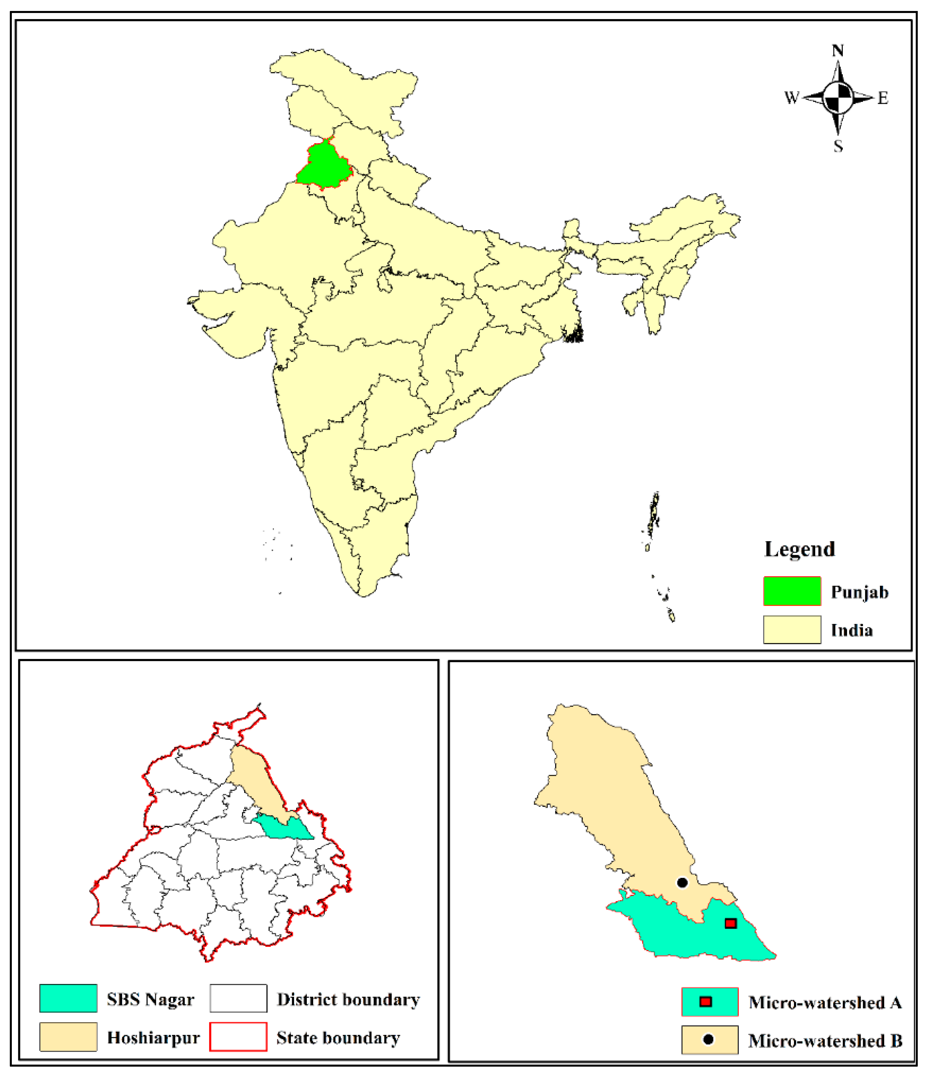
2.1. Study Areas
2.2. Hydrological Data
2.2.1. Rainfall
2.2.2. Runoff
2.2.3. Sediment Yield
2.3. Erosion-3D Model
2.4. Preparation of Model Input Files
2.4.1. Climate File
2.4.2. Soil File
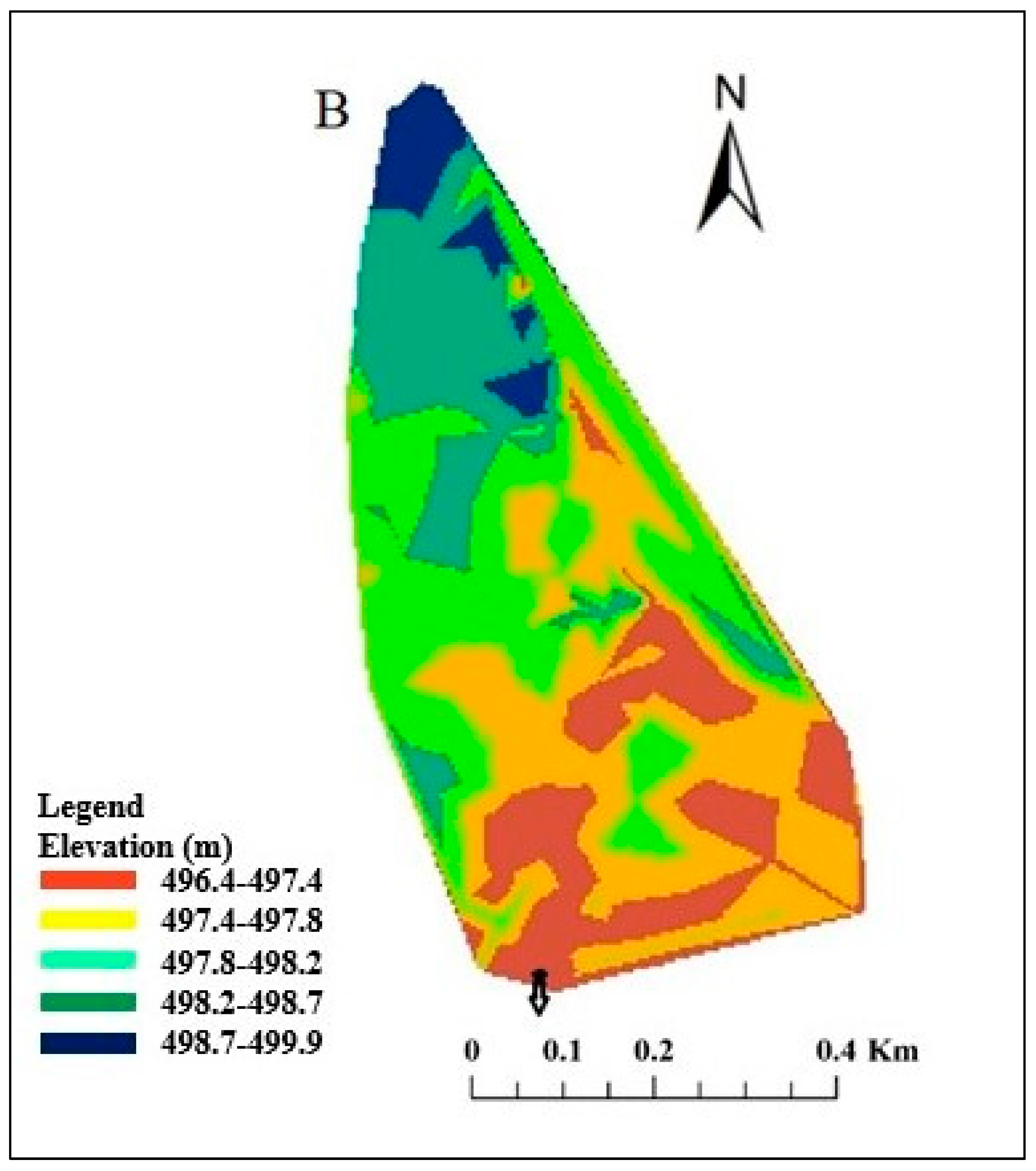
2.4.3. Relief/Slope
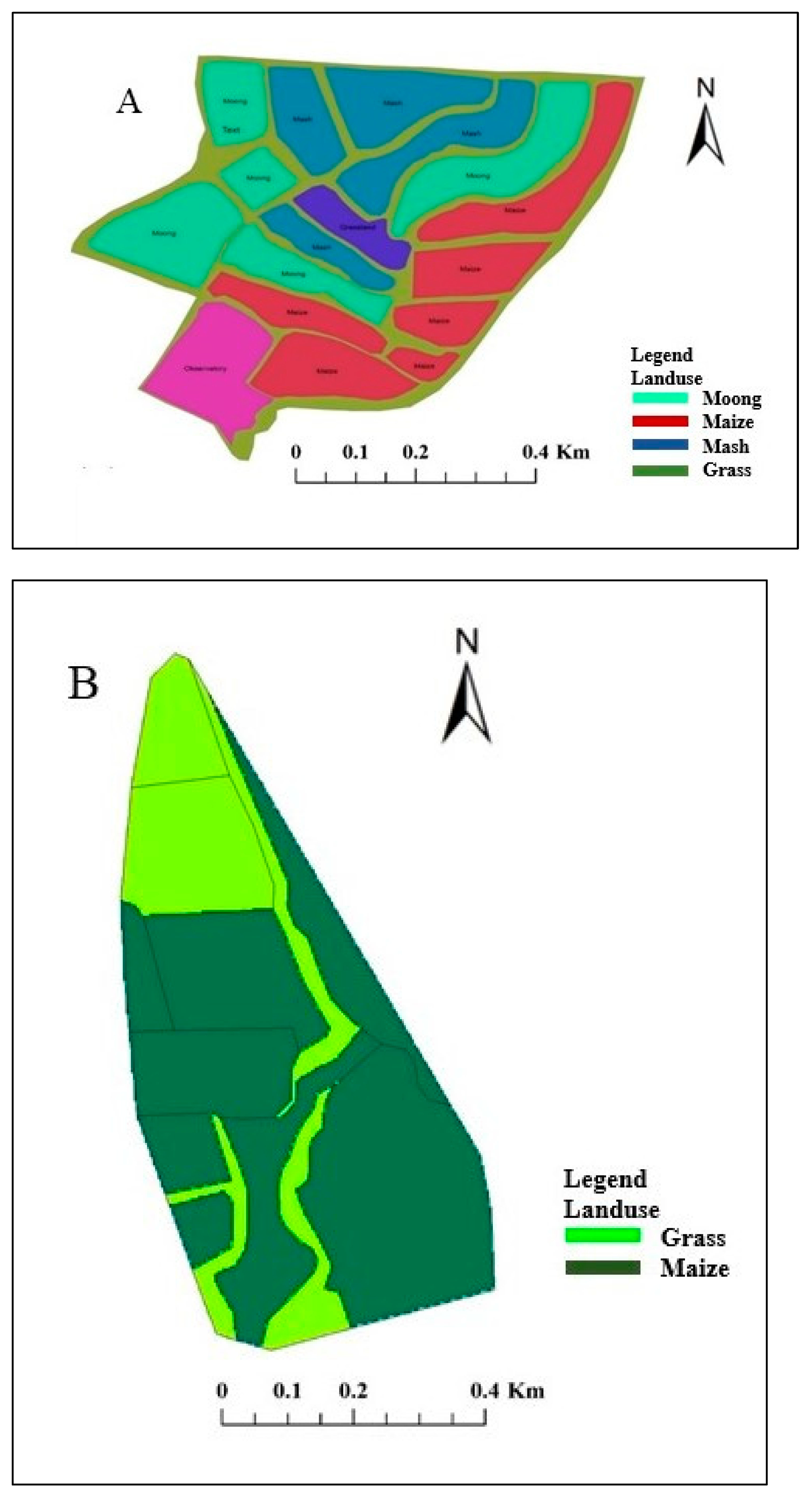
2.4.4. Land Use
2.5. Calibration and Validation of EROSION-3D Model
3. Results
3.1. Rainfall Characteristics
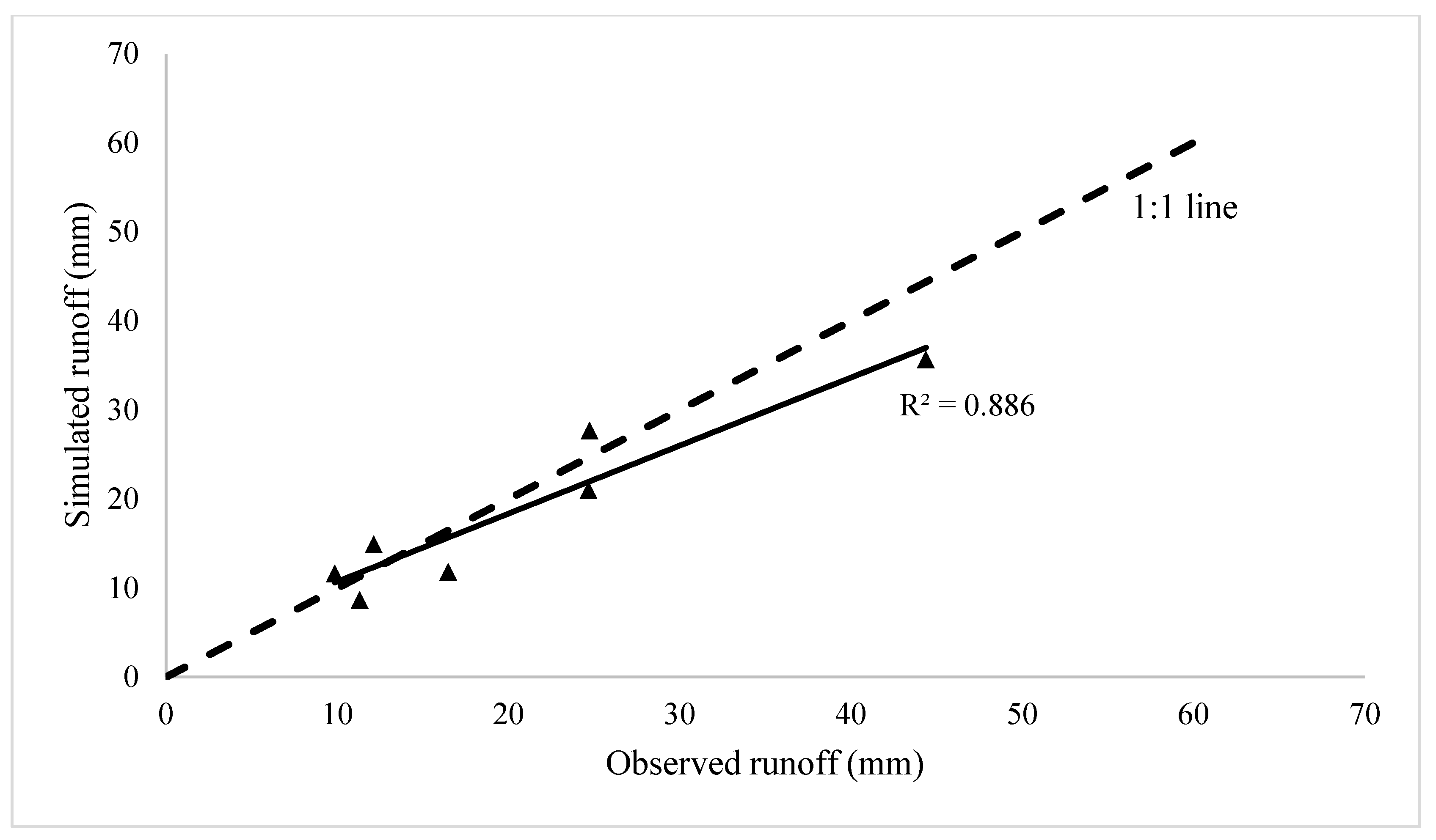
3.2. Model Calibration
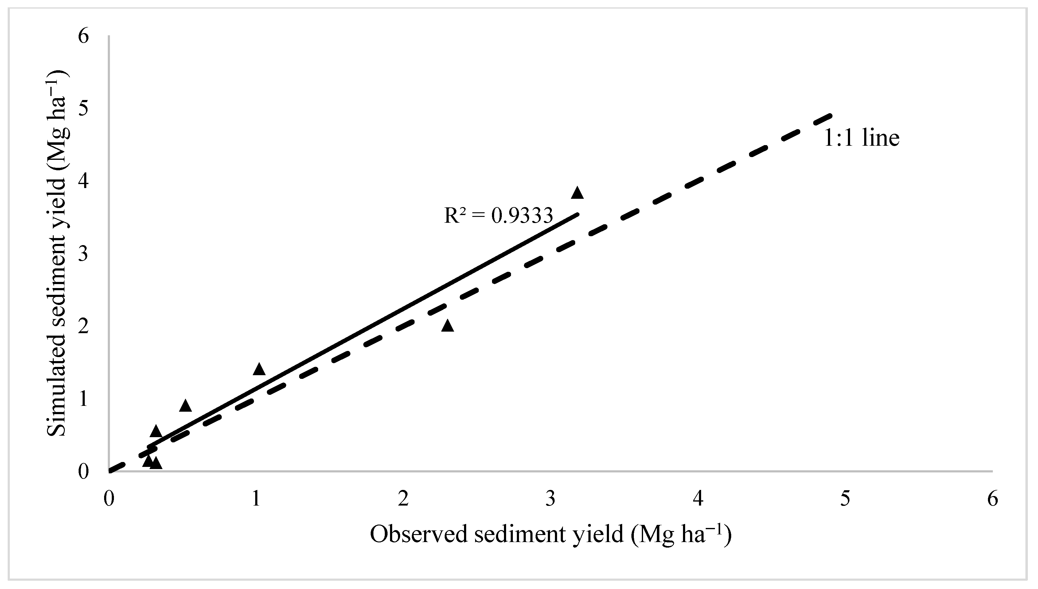
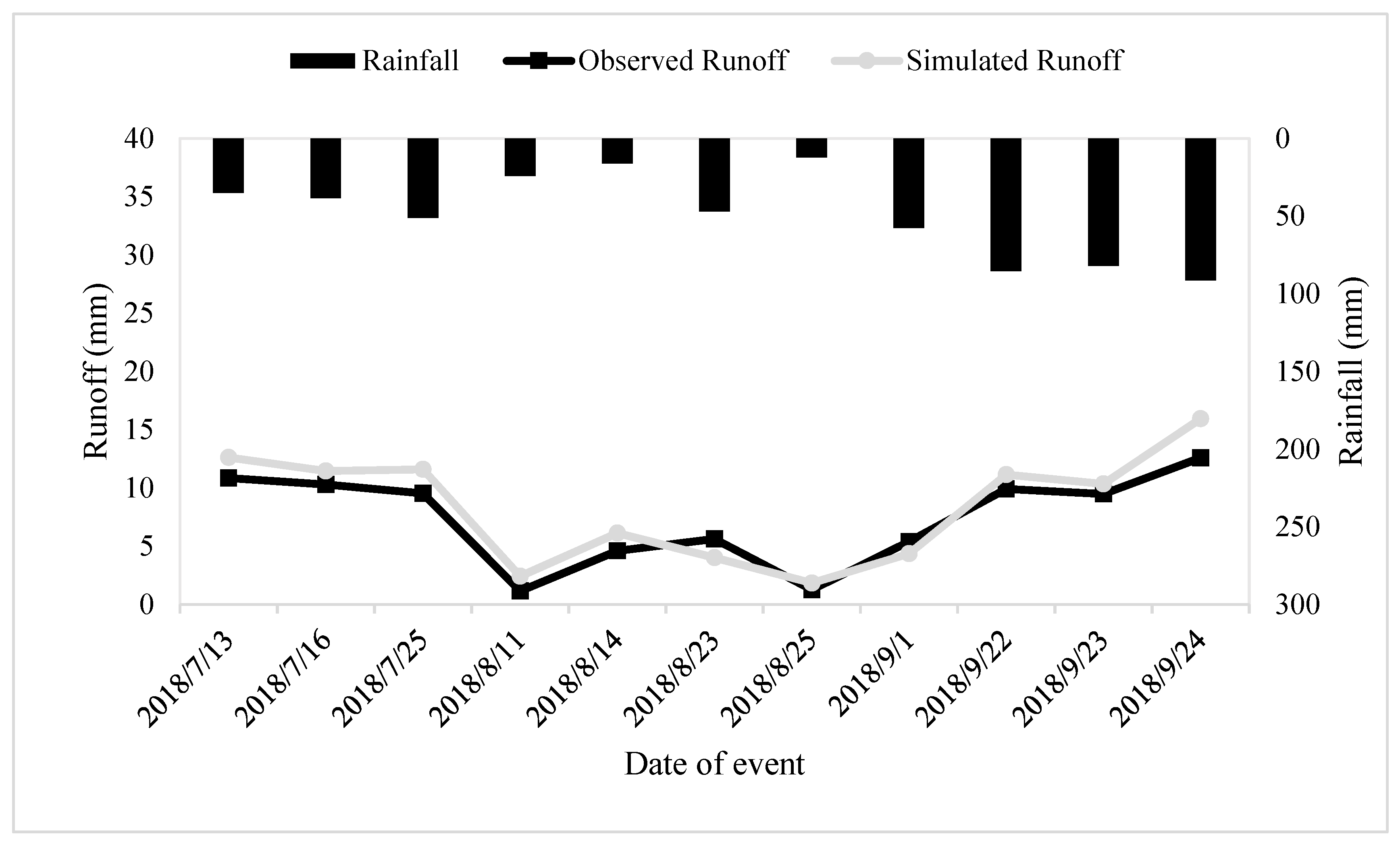
3.3. Model Validation
4. Discussion
5. Conclusions
Author Contributions
Funding
Institutional Review Board Statement
Informed Consent Statement
Data Availability Statement
Acknowledgments
Conflicts of Interest
References
- Ganasri, B.P.; Ramesh, H. Assessment of soil erosion by RUSLE model using remote sensing and GIS-A case study of Nethravathi Basin. Geosci. Front. 2016, 7, 953–961. [Google Scholar] [CrossRef] [Green Version]
- Sivakumar, M.V.K. Interactions between climate and desertification. Agric. For. Meteorol. 2007, 142, 143–155. [Google Scholar] [CrossRef]
- Mythili, G.; Goedecke, J. Economics of land degradation in India. In Economics of Land Degradation and Improvement-A Global Assessment for Sustainable Development; Nkonya, E., Mirzabaev, A., von Braun, J., Eds.; Springer: Cham, Switzerland, 2016; pp. 431–470. [Google Scholar]
- FAO; ITPS. The Status of the World’s Soil Resources (Main Report); Food and Agriculture Organization of the United Nations: Rome, Italy, 2015. [Google Scholar]
- Mohammed, A.; Alsfadi, K.; Talukdar, S.; Kiwan, S.; Hennawi, S.; Alshihabi, O.; Sharaf, M.; Harsanyie, S. Estimation of soil erosion risk in southern part of Syria by using RUSLE integrating geo informatics approach. Remote Sens. Appl. Soc. Environ. 2020, 20, 100375. [Google Scholar] [CrossRef]
- Gomiero, T. Soil Degradation, Land Scarcity and Food Security: Reviewing a Complex Challenge. Sustainability. 2016, 8, 281. [Google Scholar] [CrossRef] [Green Version]
- Dutta, S. Soil erosion, sediment yield and sedimentation of reservoir: A review. Model. Earth System Environ. 2016, 2, 123. [Google Scholar] [CrossRef] [Green Version]
- Ezz-Aldeen, M. Sedimentation and Its Challenges for the Sustainability of Hydraulic Structures. A Case Study of the Mosul Dam Pumping Station. Ph.D. Thesis, Lulea University of Technologies, Luleå, Sweden, 2020. [Google Scholar]
- Young, R.; Orsini, O.; Fitzpatrick, I. Soil degradation: A major threat to humanity. Sustain. Food Trust. A Glob. Voice Sustain. Food Health 2015, 38, 1–15. [Google Scholar]
- Bhattacharyya, R.; Ghosh, B.N.; Mishra, P.K.; Mandal, B.; Rao, C.S.; Sarkar, D.; Das, K.; Anil, K.S.; Lalitha, M.; Hati, K.M.; et al. Soil degradation in India: Challenges and potential solutions. Sustainability 2015, 7, 3528–3570. [Google Scholar] [CrossRef] [Green Version]
- Pal, S. Identification of soil erosion vulnerable areas in Chandrabhaga river basin: A multi-criteria decision approach. Model. Earth Syst. Environ. 2016, 2, 1–11. [Google Scholar] [CrossRef] [Green Version]
- ICAR. Degraded and Wastelands of India: Status and Spatial Distribution; Krishi Anusandhan Bhavan I, Pusa: New Delhi, India, 2010. [Google Scholar]
- Shardam, V.N.; Ojasvi, P.R. A revised soil erosion budget for India: Role of reservoir sedimentation and land-use protection measures. Earth Surf. Process. Landf. 2016, 41, 2007–2023. [Google Scholar] [CrossRef]
- Lal, R. Restoring soil quality to mitigate soil degradation. Sustainability 2015, 7, 5875–5895. [Google Scholar] [CrossRef] [Green Version]
- Singh, M.J.; Khera, K.L. Nomographic estimation and evaluation of soil erodibility under simulated and natural rainfall conditions. Land Degrad. Develop. 2009, 20, 471–480. [Google Scholar] [CrossRef]
- Puja, J. N.; Chadha, J. Biodiversity in the Shivalik Ecosystem of Punjab, India; PSCST-Chandigarh: Chandigarh, India, 2006; pp. 1–19. [Google Scholar]
- Kukal, S.S.; Singh, M.J. Soil erosion and conservation. In Soil Science—An Introduction; Indian Society of Soil Conservation: New Delhi, India, 2015; pp. 217–254. [Google Scholar]
- Yousuf, A.; Bhardwaj, A.; Tiwari, A.K.; Bhatt, V.K. Simulation of runoff and sediment yield from a small forest watershed in Shivalik foot-hills using WEPP model. Indian J. Soil Conserv. 2017, 45, 21–27. [Google Scholar]
- Bhardwaj, A.; Kaushal, M.P. Two- dimensional physically based finite element runoff model for small agricultural watershed: I. Model development. Hydrol. Process. 2011, 23, 397–407. [Google Scholar] [CrossRef]
- Revilla-Romero, B.; Beck, H.E.; Burek, P.; Salamon, P.; De-Roo, A.; Thielen, J. Filling the gaps: Calibrating a rainfall-runoff model using satellite-derived surface water extent. Remote Sens. Environ. 2015, 171, 118–131. [Google Scholar] [CrossRef]
- Yousuf, A.; Bhardwaj, A. Development and application of travel time based gridded runoff and sediment yield model. Int. J. Environ. Sci. Technol. 2021, 19, 1–16. [Google Scholar] [CrossRef]
- Zhang, B.; Govindaraju, R.S. Geomorphology-based artificial neural networks GANNs for estimation of direct runoff over watersheds. J. Hydrol. 2003, 273, 18–34. [Google Scholar] [CrossRef]
- Bharti, B.; Pandey, A.; Tripathi, S.K.; Kumar, D. Modelling of runoff and sediment yield using ANN, LS-SVR, REPTree and M5 models. Hydrol. Res. 2017, 48, 1489–1507. [Google Scholar] [CrossRef]
- Kim, S.; Kisi, O.; Seo, Y.; Singh, V.P.; Lee, C.J. Assessment of rainfall aggregation and disaggregation using data-driven models and wavelet decomposition. Hydrol. Res. 2016, 48, 99–116. [Google Scholar] [CrossRef]
- Sharma, N.; Zakaullah, M.; Tiwari, H.; Kumar, D. Runoff and sediment yield modeling using ANN and support vector machines: A case study from Nepal watershed. Model. Earth Syst. Environ. 2015, 1, 23. [Google Scholar] [CrossRef] [Green Version]
- Kushwaha, N.L.; Yousuf, A. Soil erosion risk mapping of watersheds using RUSLE, remote sensing and GIS: A review. Res. J. Agric. Sci. 2017, 8, 269–277. [Google Scholar]
- Werner, M.V. 2010 Data Base-Processor User Manual; Geognostic Software: Berlin, Germany, 2020. [Google Scholar]
- Schmidt, J.; Werner, M.V.; Michael, A. Application of the EROSION-3D model to the CATSOP watershed, The Netherlands. Catena 1999, 37, 449–456. [Google Scholar] [CrossRef]
- Schob, A.; Schmidt, J.; Tenholtern, R. Derivation of site-related measures to minimise soil erosion on the watershed scale in the Saxonian loess belt using the model EROSION-3D. Catena 2006, 68, 153–160. [Google Scholar] [CrossRef]
- Schindewolf, M.; Bornkampf, C.; Werner, M.; Schmidt, J. Simulation of reservoir siltation with a process-based soil loss and deposition model. Earth Planet. Sci. 2015, 10, 41–57. [Google Scholar]
- Honek, D.; Nemetova, Z.; Latkova, T. Application of physically-based EROSION-3D model for small catchment. In Proceedings of the 17th International Multidisciplinary Scientific Geo Conference SGEM, Vienna, Austria, 23 November 2017. [Google Scholar]
- Kaur, N.; Yousuf, A.; Singh, M.J. Long term rainfall variability and trend analysis in lower Shivaliks of Punjab, India. Mausam 2021, 72, 571–582. [Google Scholar] [CrossRef]
- Routschek, A.; Schmidt, J.; Kreienkemp, F. Impact of climate change on soil erosion—A high-resolution projection on catchment scale until 2100 in Saxony/Germany. Catena 2014, 121, 99–109. [Google Scholar] [CrossRef]
- Schindewolf, M.; Schmidt, J. Parameterization of the EROSION 2D/3D soil erosion model using a small-scale rainfall simulator and upstream runoff simulation. Catena 2012, 91, 47–55. [Google Scholar] [CrossRef]
- Nemetova, Z.; Honek, D.; Kohnova, S.; Hlavkova, K.; Michalkova, M.S.; Socuvka, V.; Vliskova, Y. Validation of the EROSION-3D model through measured bathymetric sediments. Water 2020, 12, 1082. [Google Scholar] [CrossRef]
- Schoeneberger, P.J.; Wysocki, D.A.; Benham, E.C.; Soil Survey Staff. Field Book for Describing and Sampling Soils, Version 3.0; Natural Resources Conservation Service, National Soil Survey Center: Lincoln, NE, USA, 2012.
- Lenz, J.; Yousuf, A.; Schindewolf, M.; Werner, M.; Hartsch, K.; Singh, M.J.; Schmidt, J. Parameterization for EROSION-3D Model under simulated rainfall conditions in lower Shivaliks of India. Geosciences 2018, 8, 396. [Google Scholar] [CrossRef] [Green Version]
- Sorooshian, S.; Gupta, V.K. Model calibration. In Computer Models of Watershed Hydrology; Singh, V.P., Ed.; Water Resources Publications: Highlands Ranch, CO, USA, 1995; pp. 23–68. [Google Scholar]
- Nash, J.E.; Sutcliffe, J.V. River flow forecasting through conceptual models. Part 1: A discussion of principles. J. Hydrol. 1970, 10, 282–290. [Google Scholar] [CrossRef]
- Nemetova, Z.; Kohnova, S.; Flodes, G. Evaluation of effect of different crop types on soil water erosion: Case study of the Myjava Hill Land, Slovakia. IOP Conf. Ser. Mater. Sci. Eng. 2019, 603, 022026. [Google Scholar] [CrossRef]
- Khokhar, A.; Yousuf, A.; Singh, M.J.; Sharma VSingh, P.S.; Gajjala, R.C. Impact of land configuration and strip-intercropping on runoff, soil loss and crop yields under rainfed conditions in the Shivalik foothills of north-west, India. Sustainability 2021, 13, 6282. [Google Scholar] [CrossRef]
- Nemetova, Z.; Kohnova, S. Comparison of sediment loss modelling by using the physically-based EROSION-3D model and the USPED empirical model: A case study of the Svacenicky Creek catchment (Slovakia). IOP Conf. Ser. Mater. Sci. Eng. 2019, 471, 022082. [Google Scholar] [CrossRef]
- Gao, J.; Bai, Y.; Cui, H.; Zhang, Y. The effect of different crops and slopes on runoff and soil erosion. Water Pract. Technol. 2020, 15, 773–780. [Google Scholar] [CrossRef]
- Geleta, I.H. Watershed Sediment Yield Modeling in Data Scarce Areas. Ph.D. Thesis, University of Stuttgart, Stuttgart, Germany, 2011. [Google Scholar]
- Dass, A.; Sudhishri, S.; Lenka, N.K.; Patnail, U.S. Runoff capture through vegetative barriers and planting methodologies to reduce erosion, and improve soil moisture, fertility and crop productivity in southern Orissa, India. Nutr. Cycl. Agroecosyst. 2011, 89, 45–57. [Google Scholar] [CrossRef]
- Singh, M.J.; Yousuf, A.; Sharma, S.C.; Bawa, S.S.; Khokhar, A.; Sharma, V.; Kumar, V.; Singh, S.; Singh, S. Evaluation of vegetative barriers for runoff, soil loss and crop productivity in Kandi region of Punjab. J. Soil Water Conserv. 2017, 16, 325–332. [Google Scholar] [CrossRef]
- Yousuf, A.; Bhardwaj, A.; Prasad, V. Simulating the impact of conservation interventions on runoff and sediment yield in a degraded watershed using the WEPP model. Ecopersia 2021, 9, 191–205. [Google Scholar]
- Yaekob, T.; Tamene, L.; Gebrehiwot, S.G.; Demissie, S.S.; Adimassu, Z.; Woldearegay, K.; Mekonnen, K.; Amede, T.; Abera, W.; Recha, J.W.; et al. Assessing the impacts of different land uses and soil and water conservation interventions on runoff and sediment yield at different scales in the central highlands of Ethiopia. Renew. Agric. Food Syst. 2020, 35, 1–15. [Google Scholar] [CrossRef] [Green Version]


| Sr. No. | Description | Micro-Watershed A | Micro-Watershed B |
|---|---|---|---|
| 1. | Latitude | 30.40° to 32.30° N | 31.36° to 31.38° N |
| 2. | Longitude | 75.30° to 75.48° E | 76.48° to 76.49° E |
| 3. | Elevation (m) | 355 | 497 |
| 4. | Slope% | 6.98 | 1.75 |
| 5. | Catchment area (ha) | 1.86 | 1.52 |
| Event No. | Rainfall (mm) | Rainfall Duration (min) | I7.5 (mm hr−1) | I15 (mm hr−1) | I30 (mm hr−1) | Total KE (MJ ha−1) |
|---|---|---|---|---|---|---|
| 1 | 55.2 | 210 | 28.2 | 51.9 | 101.1 | 8.46 |
| 2 | 71.8 | 84 | 91.8 | 149.7 | 197.7 | 13.99 |
| 3 | 34 | 42 | 53.9 | 91.6 | 186.9 | 3.46 |
| 4 | 34.8 | 63 | 79.8 | 126.6 | 190.8 | 1.06 |
| 5 | 63.1 | 112 | 67.3 | 98.4 | 139.3 | 5.03 |
| 6 | 76.2 | 210 | 40.2 | 80.4 | 146.4 | 7.49 |
| 7 | 139.6 | 194 | 57.9 | 86.1 | 120.3 | 18.19 |
| Event No. | Rainfall (mm) | Rainfall Duration (min) | I7.5 (mm hr−1) | I15 (mm hr−1) | I30 (mm hr−1) | Total KE (MJ ha−1) |
|---|---|---|---|---|---|---|
| 1 | 35.2 | 147 | 42.0 | 54.4 | 92.8 | 7.77 |
| 2 | 38.5 | 118 | 79.2 | 141.3 | 232.8 | 14.43 |
| 3 | 51.2 | 172 | 166.2 | 298.2 | 496.2 | 35.20 |
| 4 | 24.2 | 70 | 36.0 | 73.5 | 127.5 | 7.16 |
| 5 | 16.2 | 28 | 59.4 | 59.4 | 59.4 | 9.11 |
| 6 | 47.2 | 116 | 52.8 | 91.2 | 112.8 | 10.71 |
| 7 | 12.2 | 42 | 24.0 | 46.5 | 67.5 | 82.40 |
| 8 | 57.7 | 160 | 48.0 | 92.4 | 92.4 | 12.47 |
| 9 | 85.3 | 103 | 33.8 | 76.1 | 129.3 | 14.42 |
| 10 | 82.0 | 178 | 40.2 | 74.5 | 117.0 | 17.70 |
| 11 | 91.4 | 161 | 37.6 | 82.3 | 139.2 | 18.36 |
| Land Use | Skin Factor (-) | Resistance to Erosion (N m−2) | Surface Roughness (s m−1) |
|---|---|---|---|
| Maize | 0.0057 | 0.0007 | 0.024 |
| Moong and Mash | 0.138 | 0.006 | 0.075 |
| Statistical Parameters | Observed Runoff (mm) | Simulated Runoff (mm) |
|---|---|---|
| Total | 143.57 | 131.21 |
| Maximum | 44.38 | 35.65 |
| RMSE (mm) | 0.44 | |
| Mean Percent error | 4.92 | |
| Correlation Coefficient | 0.94 | |
| Model efficiency (%) | 88.0 | |
| Statistical Parameters | Observed Sediment Yield (Mg ha−1) | Simulated Sediment Yield (Mg ha−1) |
|---|---|---|
| Total | 7.93 | 9.0 |
| Maximum | 3.18 | 3.84 |
| RMSE (Mg ha−1) | 0.365 | |
| Percent Error | 12.71 | |
| Correlation Coefficient | 0.97 | |
| Model Efficiency (%) | 88.32 | |
| Statistical Parameters | Observed Runoff (mm) | Simulated Runoff (mm) |
|---|---|---|
| Total | 80.69 | 91.85 |
| Maximum | 12.59 | 15.94 |
| RMSE (mm) | 1.65 | |
| Percent Error | 21.63 | |
| Correlation Coefficient | 0.96 | |
| Model efficiency (%) | 82.77 | |
| Statistical Parameters | Observed Sediment Yield (Mg ha−1) | Simulated Sediment Yield (Mg ha−1) |
|---|---|---|
| Total | 10.66 | 12.35 |
| Maximum | 1.72 | 1.96 |
| RMSE (Mg ha−1) | 0.19 | |
| Percent Error | 17.16 | |
| Correlation Coefficient | 0.97 | |
| Model Efficiency (%) | 74.48 | |
Publisher’s Note: MDPI stays neutral with regard to jurisdictional claims in published maps and institutional affiliations. |
© 2022 by the authors. Licensee MDPI, Basel, Switzerland. This article is an open access article distributed under the terms and conditions of the Creative Commons Attribution (CC BY) license (https://creativecommons.org/licenses/by/4.0/).
Share and Cite
Singh, M.; Yousuf, A.; Singh, H.; Singh, S.; Hartsch, K.; von Werner, M.; Almaliki, A.H.; Elnaggar, A.Y.; Hussein, E.E.; Ali, H.R. Simulation Accuracy of EROSION-3D Model for Estimation of Runoff and Sediment Yield from Micro-Watersheds. Water 2022, 14, 280. https://doi.org/10.3390/w14030280
Singh M, Yousuf A, Singh H, Singh S, Hartsch K, von Werner M, Almaliki AH, Elnaggar AY, Hussein EE, Ali HR. Simulation Accuracy of EROSION-3D Model for Estimation of Runoff and Sediment Yield from Micro-Watersheds. Water. 2022; 14(3):280. https://doi.org/10.3390/w14030280
Chicago/Turabian StyleSingh, Manmohanjit, Abrar Yousuf, Harpreet Singh, Sukhdeep Singh, Kerstin Hartsch, Michael von Werner, Abdulrazak H. Almaliki, Ashraf Y. Elnaggar, Enas E. Hussein, and Hager R. Ali. 2022. "Simulation Accuracy of EROSION-3D Model for Estimation of Runoff and Sediment Yield from Micro-Watersheds" Water 14, no. 3: 280. https://doi.org/10.3390/w14030280