Spatiotemporal Characteristics Analysis and Driving Forces Assessment of Flash Floods in Altay

Abstract

Flash floods are devastating natural disasters worldwide. Understanding their spatiotemporal distributions and driving factors is essential for identifying high risk areas and predicting hydrological conditions. In this study, several methods were used to analyze the changing patterns and driving factors of flash floods in the Altay region. Results indicate that the number of flash floods each year increased in 1980–2015, with two sudden change points (1996 and 2008), and April, June, and July presented the highest frequency of events. Habahe and Jeminay were known to have high flash flood incidences; however, currently, Altay City, Fuhai, Fuyun, and Qinghe are most affected. In terms of driving force analysis, precipitation and altitude performance have a key impact on flash flood occurrence in this settlement compared to other subregions, with a high percentage increase in the mean squared error value of 39, 37, 37, 37, and 33 for 10 min precipitation in a 20-year return period, elevation, 60 min precipitation in a 20-year return period, 6 h precipitation in a 20-year return period, and 24 h precipitation in a 20-year return period, respectively. The study results provide insights into spatial–temporal dynamics of flash floods and a scientific basis for policymakers to set improvement targets in specific areas.

1. Introduction

Flash floods are disaster events with high peak flows and short response times in mountainous watersheds of tens to numerous square kilometers, usually triggered by heavy rainfall [1,2]. Globally, flash floods are among the most devastating natural disasters, often resulting in loss of life and significant economic damage [3]. In America, for example, flash floods ranked first among the causes of death, with approximately 100 deaths every year [4]. Additionally, between 1950 and 2006, 40% of flood related deaths in Europe were from flash floods [5], while this proportion exceeded 80% in southern Europe [6]. China is a vast country with a complex ecological and geographical environment, which is also influenced by heavy precipitation, human activities and other factors [7]. China has suffered the most serious flash floods worldwide [8], and the incidence of these events shows an upward trend [9]. From a regional point of view, affected by the complex terrain, the distribution of heavy rainfall presents an obvious spatial difference pattern. Indeed, according to the latest IPCC report, under a global warming scenario of 1.5 °C, flash floods will be more frequent and more violent in Asia [10]. Meanwhile, the Altay ecosystem is extremely sensitive to climate change and human activity owing to its vulnerability and geographical conditions. From this perspective, it is crucial to bridge the knowledge gap between the spatial and temporal patterns of flash floods and the driving patterns in the Altay region.

In recent decades, most relative studies have illustrated that flash floods are related to a combination of spatial and temporal factors [11,12,13,14]. Currently, research on flash floods has concentrated on three aspects: (1) the assessment of flash flood risk [15,16], (2) flash flood mechanisms [17,18], and (3) spatiotemporal distribution and influencing factors [19,20]. The risk assessment of flash floods is mainly to identify high and low risk areas at the local or national scale [15,21,22], which are mainly quantified by three methods: the scenario simulation method [23,24], a historical data based method [25,26], and an index based system method [27,28]. Additionally, the complexity of flash flood formation has led many of these studies to be conducted only in typical watersheds [29]. In general, when researching flash flood disasters, it is necessary to make a comprehensive record of past events. According to this theory, it is very meaningful to analyze the temporal and spatial components of flash flood disasters and explore the driving factors behind them. Concerning spatial–temporal distribution and influencing factors, numerous studies have used kernel density estimation, spatial autocorrelation, spatial gravity center migration, and standard deviational ellipse to discover the temporal and spatial specialties of flash floods [8,30]. Numerous methods have been applied to conduct the driving force analysis of flash floods (i.e., principal component analysis, geographical detector, multiple linear regression, and random forest), each with its advantages. On this basis, precipitation, terrain, normalized difference vegetation index (NDVI), and human activities, among others, have been selected by many scholars as influencing factors [31]. This type of study generally selects a country (or province) as the study object.

Despite extensive research into the mechanisms and drivers of flash floods, problems remain. Firstly, some studies indicate that land use has changed dramatically due to urban expansion and increased human activity [20], and there is an urgent need for research that starts with land-use factors for driving force analysis. Second, certain static factors respond to dynamic factors, while ignoring the spatiotemporal aspects of dynamic factors, which may lead to inaccurate and objective results. Current studies on the influences of flash floods on urban expansion and human activities and intensification of rainfall are needed, although some studies have explained the response mechanisms between human activities and flash floods. Moreover, some previous studies were performed to detect only the interaction between two drivers [31,32], but they did not adequately reflect the rate of contribution of each driver in the different models. Finally, the current flood prediction research is mostly focused on areas with high flooding [33,34], while ignoring arid areas such as Altay. However, the past flash flood disasters in Altay also caused great harm to local people and economic losses. In particular, with the influence of the Altay Mountains and the Gurbantunggut Desert, the geological features of Altay show uniqueness and climate diversity; thus, there is an urgent need to explore and analyze the spatial-temporal distribution and driving factors of flash floods in Altay.

The purpose of this research is to analyze the changing patterns of historical flash floods and explore the driving factors behind flash floods in the Altay region. The primary objectives were: (1) discovering the spatial–temporal variability of flash floods based on the M-K test, kernel density estimation, standard deviational ellipse, and spatial gravity center model; and (2) analyzing the drivers of flash flooding in four land-use type subdivisions using four methods. The research results can provide scientific reference and decision support for the development of reasonable disaster prevention measures and effective flood risk management.

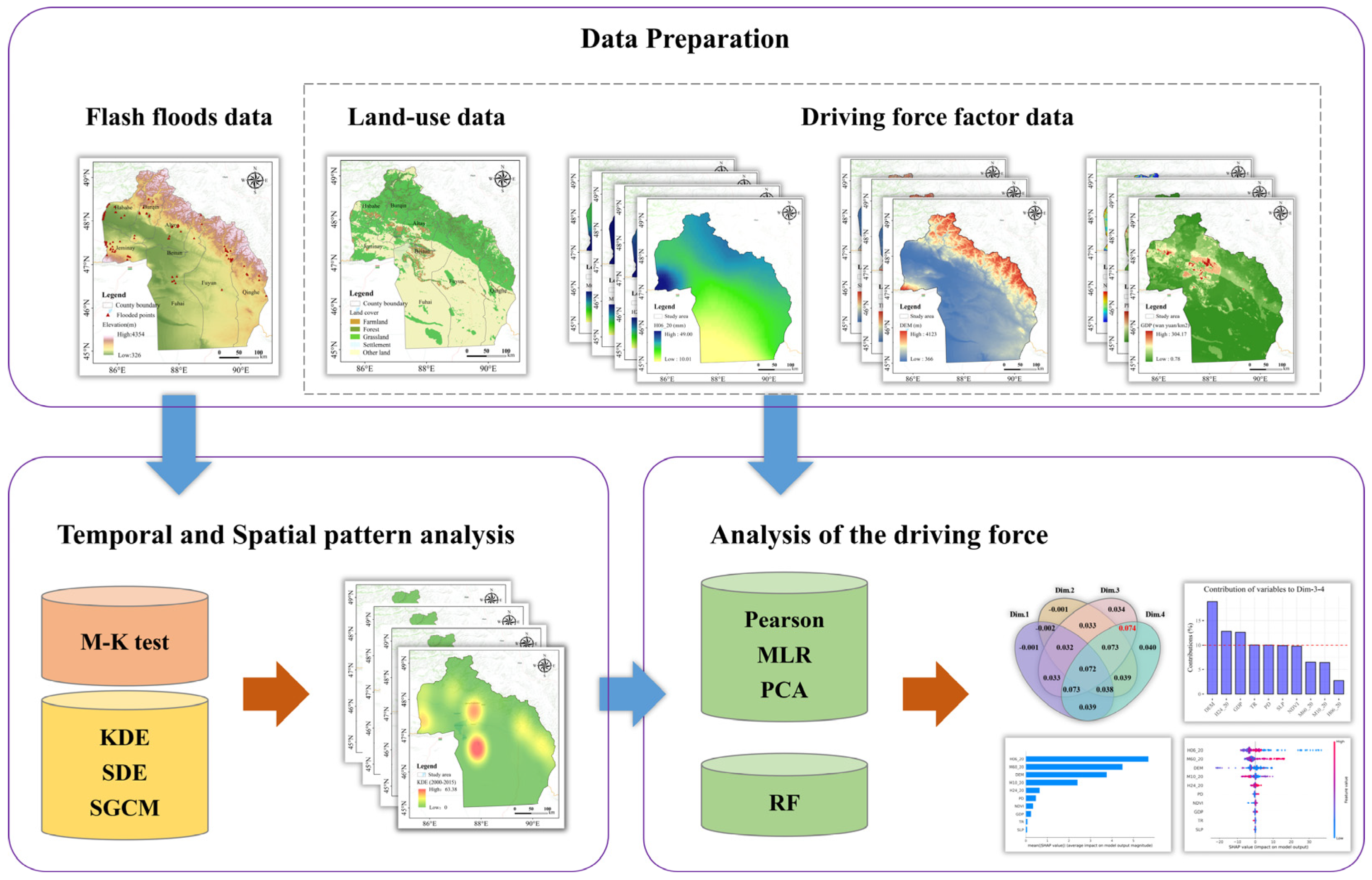
2. Materials and Methods

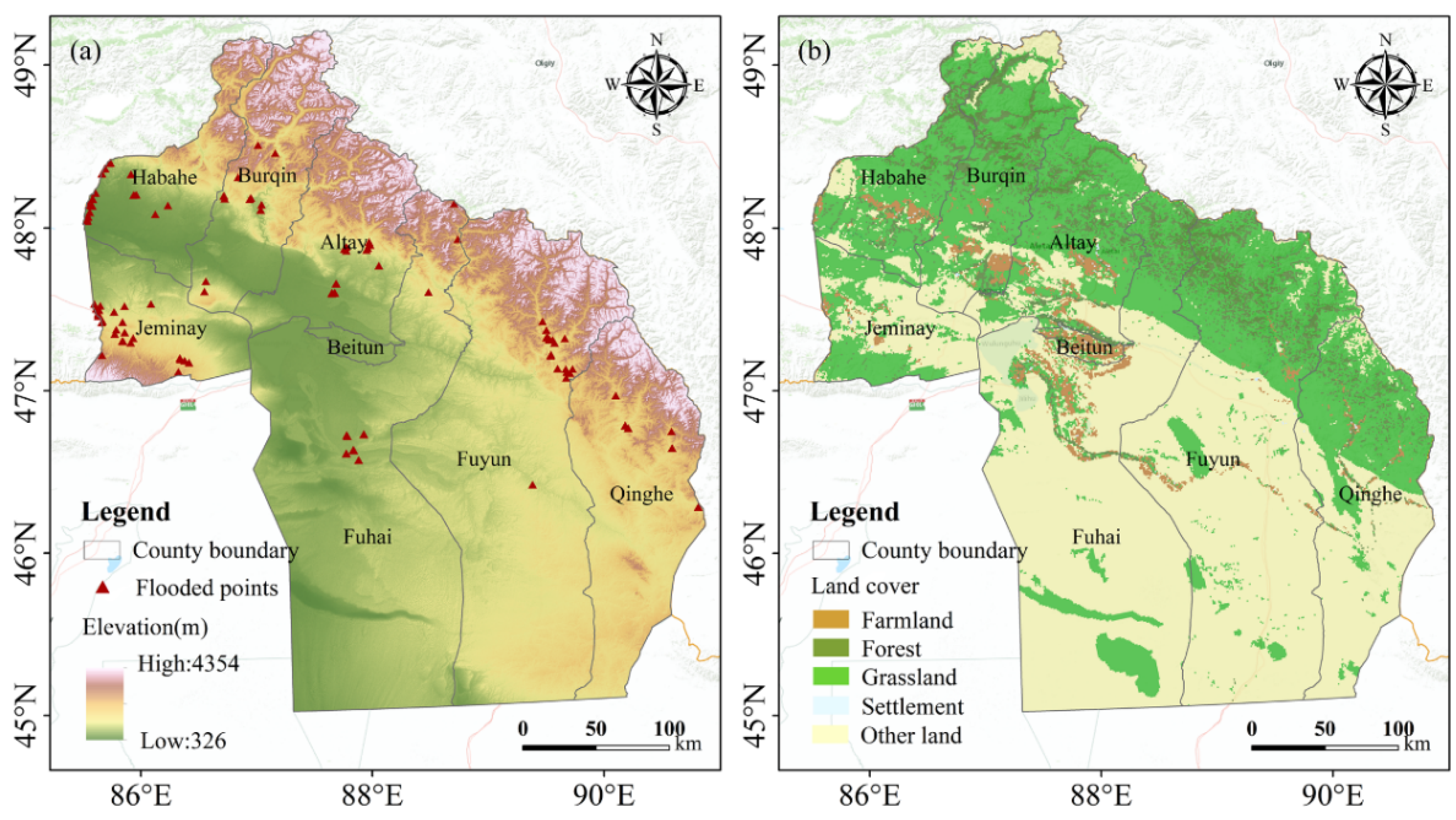
2.1. Study Area

The Altay Prefecture is located in the heartland of Eurasia, spanning over 45°0000″–49°1045″ N and 85°3136″–91°0423″ E. The area is in northwest China, bordered by Mongolia, Russia, and Kazakhstan. The Altay Prefecture is composed of seven counties and covers 1.18 × 10⁵ km². Precipitation and temperature in the Altay Prefecture vary considerably. Owing to the blockage of the Arctic and Atlantic monsoons by the Altay Mountains, high precipitation and low temperatures occur in the northern mountains. Meanwhile, the southern plain has a dry climate and scarce precipitation because of the effect of the Gurbantunggut Desert. A flash flood is a violent surface water runoff event, which is usually caused by precipitation in a small watershed. According to the flash floods inventory database provided by National Mountain Flood Disaster Investigation Project (NMFDIP), the spatial distribution of flash floods in 1980–2015 is plotted in Figure 1. The position of flash flood points is defined as the central location of the historical flash flood ditch.

Affected by hydrothermal conditions, climate change, and human activities, the land cover in 2020 is mainly cropland (1.91%), forest (4.92%), grassland (11.39%), meadow (10.94%), and desert (61.84%). Altay is one of the key pastoral areas in China, with rich natural grassland resources accounting for nearly 15% of the Xinjiang Uygur Autonomous Region, where flash floods are rapidly increasing, posing a serious threat to people’s lives and property.

2.2. Dataset

Flash floods can be caused by a variety of factors, such as heavy rainfall, dam and levee breaches, landslides, and urbanization [35], but heavy rainfall is generally considered to be the most common cause, and in this study, heavy rainfall is the factor of flash floods. Previous studies have shown that factors such as precipitation, topography, and human activities are closely related to the occurrence of flash floods [11,36]. Therefore, the scientific data used in this research are mainly divided into two types: (1) Flash floods inventory database, which is provided by NMFDIP, which was launched by the Ministry of Water Resources of China and the Ministry of Finance of China (MWRCMFC) in 2013. Collected by field surveying, the dataset records the occurrence time, longitude, latitude, and other attributes of historical flash floods. It is worth mentioning that not every cause of flash floods is mentioned in this database, however, among the causes mentioned in this study, the main factor of flash floods in Altay is heavy rainfall. This database had been strictly inspected, and widely used in a large number of studies [37,38,39]; and (2) The cover raster data and the driving force factor, which is consistent with previous studies in selecting driving factors, mainly including precipitation factors, representing topography and human activities data. Precipitation data is grid data with four indicators, which are the 6 h rainstorm (H06_20), 24 h rainstorm (H24_20), 10 min rainstorm (M10_20), and 60 min rainstorm (M60_20) in the 20-year return period. This dataset belongs to the flood inventory dataset mentioned above and is also widely used. Data representing topography are digital elevation model (DEM) raster data and its derivatives (slope raster data (SLP) and topographic relief raster data (TR)). NDVI, gross domestic product (GDP), and population density (PD) data were used to represent human activities.

According to the description of the above data, we determine that the number of historical flash flood points in Altay is 210, from the flash flood database. Precipitation raster data of 1 km × 1 km is derived from the inverse distance weighted interpolation of the precipitation factor grid. We calculate the TR and SLP based on DEM data using the focal statistical method. The NDVI raster data is the multi-year average value of MODIS NDVI products (MOD13A1) from 2000 to 2015, calculated from the Google Earth Engine platform. The corresponding historical PD and GDP raster data are obtained from the Resource and Environment Science and Data Center of the Chinese Academy of Sciences (RESDC). More descriptions of the datasets are represented in

Table 1. Data source and description.

Type	Factors	Spatial Resolution	Temporal Resolution	Description
Basic data	Flash floods	Vector data	1980–2015	China, National Mountain Flood Disaster Investigation Project [31].
	Landcover	1 km × 1 km	2010	RESDC.
Driving force factor data	Precipitation factors	Vector data	2015	China, National mountain flash flood disaster survey and evaluation data.
	DEM	90 m × 90 m	2010	Geospatial Data Cloud of China.
	NDVI	1 km × 1 km	2000–2015	Google Earth Engine.
	Population density	1 km × 1 km	2000, 2005, 2010 and 2015	RESDC.
	GDP	1 km × 1 km	1995, 2000, 2005, 2010 and 2015	RESDC.

and shown in Figure 2.

3. Methods

3.1. Spatiotemporal Analysis Method

3.1.1. Temporal Analysis

Proposed by Kendall in 1979, The Mann–Kendall (M-K) test is a mature method, which is widely used in the studies of hydrology, meteorology, and natural disasters [37,38]. Thus, the M-K test method was used in this study to recognize the mutation point and the trend in the temporal variation of flash floods from 1980 to 2015. Specifically, annual is used as the time scale, and the entire Altay region is used as the spatial scale, and the mutation point and the changing trends were detected. The time node when the occurrence of flash floods changed significantly can be revealed by mutation point. The M-K test can obtain two results for UF and UB. The UF expresses the trend of flash floods over time in a normal time series. The UB is the statistical sequence obtained from the inverse time series. When UF is greater than 0, the occurrence of flash floods shows an upward trend. Conversely, is a downward trend. If the value of UF exceeded the critical line (p = 0.05), it indicates that the rising or falling trend was significant. Draw UF and UB into a curve, and the intersection of the two lines is the mutation point in the time series [30]. Flash flood detailed information can be found in a previous study [39].

3.1.2. Spatial Analysis

(1)

Estimation of the kernel density, KDE

Here, the kernel density estimation technique is used to create a representation of flash floods, for the kernel function allows this estimate to be considered as the average of the effects of the kernel function, which is centered on the flash flood location and evaluated at each point. Using kernel density estimation, we calculated the spatial intensity of flash floods as follows:

$${\lambda }_h\left(P\right)=\frac{1}{nh}{\displaystyle \sum }_{i=1}^{n}m\left(\frac{P-P_i}{h}\right)$$

(1)

where λ_h(P) represents the probable spatial intensity of flash floods, and m(.) is the kernel function, which is an invariant function but not necessarily a positive function, P₁, …, P_n represents the location of n of the observed flash floods, and h is the bandwidth, which determines the semidiameter of the circle centered at P. The spatial density of flash floods was calculated for kernel density estimation using ArcGIS 10.6 [40].

(2)

Standard deviational ellipse, SDE

The standard deviation ellipse is always used as a general purpose GIS tool for measuring binary distribution features. The tool is typically used to depict trends in the spatial distribution of elements by summarizing the direction and dispersion of elements. When the flash flood data are presented as points, the direction and trends were generally determined by SDE method. Based on ArcGIS10.6, the SDE is mainly influenced by three main factors, namely, mean location, the concentration or dispersion of features, and direction. Additionally, the SDE can be expressed as one to three standard deviations, in this study, one standard deviation was used [41].

(3)

Spatial gravity center model, SGCM

The spatial center of gravity model facilitates the study of the spatiotemporal migration of elements by analyzing their center of gravity trajectories. Here, the distribution of factors in two-dimensional space and their evolutionary characteristics are revealed directly and precisely with this model [42]. On this basis, we calculated the coordinates of the center of gravity and the average annual precipitation for flash floods [43]. The coordinates of the center of gravity of flash floods are as follows:

$$G_f\left(x\right)=\frac{{{\displaystyle \sum }}_1^n{f}_i\left(x\right)}{n},G_f\left(y\right)=\frac{{{\displaystyle \sum }}_1^n{f}_i\left(y\right)}{n}$$

(2)

where G_f(x) and G_f(y) denote the center of gravity coordinates of annual flash floods, n denotes the number of annual flash floods, while f_i(x) and f_i(y) denote the geometric coordinates of the ith flash flood (i = 1, 2, …, n) [44]. In addition, the center of gravity coordinates of the average annual precipitation was as follows:

$$G\left(x\right)=\frac{{{\displaystyle \sum }}_{i=1}^n{x}_i\times m_i}{{{\displaystyle \sum }}_{i=1}^n{m}_i},G\left(y\right)=\frac{{{\displaystyle \sum }}_{i=1}^n{y}_i\times m_i}{{{\displaystyle \sum }}_{i=1}^n{m}_i}$$

(3)

where G(x) and G(y) denote the annual center of gravity coordinates of this element (annual average precipitation), (x_i, y_i) denotes the geometric coordinates of the ith weather station for annual average precipitation, and m_i is the attribute value of the ith weather station [42].

3.2. Analysis of Influencing Factors

In this section, we will discuss the influencing factors of flash floods based on land use cover change data. Since all historical flash floods occurred in grassland, settlement, farmland, and forest areas, we chose these four types of land cover. Due to the vast area of the Altay region, 1000 random points in each subregion were selected as the sample points. Then, we could take these point value data to explore the influence mechanism between mountain flash floods and driving forces factors under different land use. The correlation and interaction between influencing factors and kernel density, the weight of influencing factors, and their contribution to the flash flood will be analyzed and quantified. Finally, 210 flood points and non-flood point data were selected to analyze the driving factors of disaster points using a random forest.

3.2.1. Correlation Coefficient Calculation

The Pearson correlation coefficient [45] is a classical method to measure the linear correlation of x and y. This coefficient is the product of the covariance of the two variables divided by their standard deviation, essentially making it is a standardized measurement of covariance such that the result is always between −1 and 1. This statistic is denoted as:

$$r_{xy}=\frac{{\displaystyle {\sum }_{i=1}^n(x_i-\overline{x})(y_i-\overline{y})}}{\sqrt{{\displaystyle {\sum }_{i=1}^n{(x_i-\overline{x})}^2}}\sqrt{{\displaystyle {\sum }_{i=1}^n{(y_i-\overline{y})}^2}}}$$

(4)

where $r_{xy}$ is the correlation coefficient of the two sets of data $x$ and $y$. $x_i$ and $y_i$ represent the corresponding values indexed in $i$, respectively. Here, $\overline{x}$ and $\overline{y}$ are the mean of each list data; n is the size of the samples. The $r_{xy}$ values and corresponding correlation levels are listed in

Table 2. Classification of the range level of Pearson correlation coefficient.

${\mathit{r}}_{\mathit{x}\mathit{y}}\mathbf{Value}$	Relevance
$r_{xy}=0$	no association or no correlation
$0<\left|r_{xy}\right|<$0.25	very weak correlation
$0.25<\left|r_{xy}\right|<0.5$	weak correlation
$0.5<\left|r_{xy}\right|<0.75$	strong correlation
$0.75<\left|r_{xy}\right|<1$	very strong correlation
$\left|r_{xy}\right|=1$	perfect correlation

[46].

3.2.2. Multiple Linear Regression, MLR

A phenomenon is often related to multiple factors; therefore, multiple linear regression statistical methods are involved. The goal of multiple linear regression is to establish a linear relationship model between the explanation (independent variable) and response (dependent variable). The MLR equation is as follows:

$$y_i={\alpha }_0+{\alpha }_1{x}_{i1}+{\alpha }_2{x}_{i2}+\dots {\alpha }_p{x}_{ip}+\epsilon (i=1,2,\dots n)$$

(5)

where $y_i$ represents the dependent variable; $x_i$ represents the explanatory variable. ${\alpha }_0$ is the constant term; ${\alpha }_p$ is the slope coefficient for each explanatory variable, and $\epsilon$ is the residual term of the MLR.

3.2.3. Principal Component Analysis, PCA

The essence of PCA [45] is to find the most important aspect of the data through orthogonal transformation and use the most important aspect to replace the original data. For a set of data that may have a linear correlation between different dimensions, PCA can transform this set of data into data that are linearly independent of each dimension through orthogonal transformation. It is a dimensionality reduction method of unsupervised learning. It only needs eigenvalue decomposition to compress and denoise data. PCA mainly has the following three advantages: it only needs to measure the amount of information by variance, not that affected by factors other than the data set; the orthogonal between the principal components can eliminate the mutual influence factors between the original data components; and the calculation model is considered to be simple, and the main operation is eigenvalue decomposition, which is easy to implement.

3.2.4. “Random Forest”, RF

Random forest, as the name suggests, is to build a forest randomly. There are many decision trees but there is not a correlation between each decision tree in the random forest. Random forest is a method that uses multiple classification trees to distinguish and classify data. While classifying the data, it can also give the importance score of each variable (gene), and evaluate how each variable is the role played in classification. The following technique was implemented in the R package “random forest” [47].

It has many advantages: it is not easy to fall into overfitting and has good antinoise ability; it can handle relatively high dimensional data without feature selection and has strong adaptability to data sets. It can handle discrete data, process continuous data, and does not need to be standardized. In the training process, the mutual influence between features can be detected, and the implementation is relatively simple.

SHAP, whose name comes from SHapley Additive ExPlanation, originated from cooperative game theory. It is inspired by cooperative game theory to construct an additive explanatory model, and all features are regarded as contributions. For each prediction sample, the model produced a prediction value, and the SHAP value was the value assigned to each feature in the sample. The SHAP value is given by the following equation:

$$y_i=y_{base}+f\left(x_{i1}\right)+f\left(x_{i2}\right)+\dots +f\left(x_{ij}\right)$$

(6)

where $j$ is the number of features; $x_{ij}$ is the jth feature of the ith sample; $y_i$ is the predicted value of the model for the sample; $y_{base}$ is the baseline for the entire model; $f\left(x_{ij}\right)$ is the SHAP value of $x_{ij}$. If $f\left(x_{ij}\right)>0$, it means that the feature improves the predicted value and has a positive effect. On the contrary, it indicates that the feature reduces the predicted value, which has a negative effect. Compared with the traditional feature importance calculation method, the SHAP value can reflect the influence of the characteristics in each sample, while also showing a positive and negative effect.

The technical flowchart of this study is drawn based on the data and methods previously presented (Figure 3). First, based on the mountain torrent data, the MK test is used to analyze the time scale, and the KDE, SDE, and SGCM are used to analyze the space scale, and the results of the time–space analysis are obtained. Second, the kernel density estimation results and the mountain torrent driving force factor data are combined, and the Pearson coefficient calculation, PCA, and MLR are used to obtain the interaction and contribution rate of the influence factors; the RF and SHAP value are used to show how each variable affects the mechanism of torrents.

4. Results

4.1. Temporal Pattern of Flash Floods

As shown in Figure 4, the variation characteristics of flash floods in the time series from 1980 to 2015 were expressed in period scale, yearly scale, and monthly scale. As shown in Figure 4b, the intersection of UF and UB occurred in 2008, indicating that 2008 was the mutation point of a flash flood. In addition, the trend of UF indicated an almost constant increase in flash floods after 1996. Thus, 1996 is also an important time point. According to the result of the M-K test in Figure 4b, the occurrence of flash floods in the yearly scale was divided into three time periods, which are 1980–1996, 1997–2008, and 2009–2015, when the number of flash floods was 18, 78, and 112. Figure 4a indicated that few flash floods occurred during the first period, except in 1995. In the second period, the number of flash floods increased, especially in 1997, 1998, and 2002. The number of flash floods in the third period continued to increase, peaking at 56 in 2013. The results of the M-K test indicated that the year 2008 is the mutation point (the intersection point of UF and UB), and it indicated that the number of flash floods steadily increased after 2008, which was consistent with the statistical results. In addition, the value of UF steadily increased after 1996, indicating that the frequency of flash floods rose after 1996. Figure 4c shows that the most flash floods occurred in July, accounting for 37.5%. April and June also had many flash flood records. No flash floods occurred in January, February, October, November, and December.

4.2. Spatial Pattern of the Flash Floods

The kernel density analysis results are presented in Figure 5. In the 1980–1996 period, Habahe (13 flash floods) was the area with the most frequent occurrence of flash floods. Altay City had two flash floods, and other districts had very few flash floods (Figure 5a). In the period from 1997–2008, the high frequency of flash floods was concentrated in Habahe (44 flash floods) and Jeminay (12 flash floods), and Burqin had 5 flash floods. In addition, the frequency of flash floods has increased significantly in the period from 2007 to 2015. The number of flash floods in Habahe (9 flash floods) and Jeminay (11 flash floods) decreased. A high frequency of flash floods occurred in Altay City (24 points) and Fuhai (30 points). Fuyun (14 points) and Qinghe (22 points) showed an increase (Figure 5c). In general, the area with a high incidence of flash floods was concentrated early on in Habahe and more recently in Altay City.

According to the results of the standard deviational ellipse analysis (Figure 6a,b). The regions with spatial unbalance were mainly distributed in Fuyun and Qinghe from the period to 1980–1996 and 1997–2008. From 1997–2008 to 2009–2015, the occurrence of flash floods became relatively uniform. In general, the orientation and trend of standard deviational ellipses show that more flash floods spread to the southeast of the Altay Prefecture. In addition, according to the evolution track of the gravity center, the displacement of the flash flood gravity center from 1997–2008 to 2009–2015 indicates that the distribution of flash floods has changed significantly. The result of the evolution track of the gravity center is consistent with the result of the standard deviation ellipse.

4.3. Analysis of the Driving Force of Mountain Flash Flood Kernel Flood

The correlation coefficient and p-value between each influencing factor with the kernel density of flash floods in four land cover subregions are listed in

Table 3. Correlation coefficient $r_{xy}$ and multiple linear regression p-value in the different subregions of the land cover.

Factors	Farmland		Forest		Grassland		Settlement
	r	p	r	p	r	p	r	p
H06_20	0.030	0.563	−0.580	<0.001	0.084	0.007	0.351	0.007
H24_20	−0.238	<0.001	0.445	0.068	0.470	<0.001	0.105	<0.001
M10_20	−0.152	<0.001	−0.426	<0.001	−0.052	<0.001	0.100	<0.001
M60_20	0.047	<0.001	−0.497	<0.001	0.133	0.002	0.371	<0.001
DEM	0.107	<0.001	−0.377	0.196	−0.176	0.255	0.263	0.179
SLP	0.007	0.719	−0.248	0.037	−0.149	0.945	0.144	0.373
TR	0.002	0.981	−0.247	0.111	−0.147	0.883	0.138	0.384
NDVI	0.008	0.543	−0.188	<0.001	0.064	<0.001	−0.086	<0.001
GDP	0.122	<0.001	0.227	<0.001	0.130	<0.001	0.154	<0.001
PD	0.181	<0.001	0.265	<0.001	0.221	<0.001	0.212	<0.001

. The interaction between driving factors is shown in Figure 7. We can take Figure 7a,b as examples to explain the specific implementation steps and meanings of the image. The four dimensions in subpicture (a) are the first four principal components of the variable data principal component transformation, and the cumulative contribution rate has reached more than 85%. The number represents the R-squared between the dimensional combination model and the variable data. We know that the R-squared is used to measure the similarity between the regression problem in the linear regression problem. The larger the R-squared, the better the model fitting effect. Therefore, we choose the Dim 3 and 4 whose corresponding largest R-squared is 0.074. Subpicture (b) shows the contribution rate of each variable factor to the model. The model is the linear model that we choose to consist of Dim 3 and 4.

The first is farmland. The factors that passed the significance test and have a slight correlation included H24_20 (r = −0.238, p < 0.001), PD (r = 0.181, p < 0.001), and M10_20 (r = −0.152, p < 0.001). The highest adjusted R-squared value of MLR for the first four principal components (accumulative contribution rate was 0.87) was 0.074, which came from Dim-3-4. The variable factors with higher contribution were DEM (18.92%), H24_20 (12.85%), and GDP (12.65%).

The second was the forest subregion. The correlation coefficient r value of some factors was higher than in the forest, including H06_20 (r = −0.580, p < 0.001), M10_20 (r = −0.426, p < 0.001), M60_20 (r = −0497, p < 0.001). The interaction of Dim-1-2-3-4 contributed the highest adjusted R-squared value and the variables that were higher than the mean value include PD (11.04%), GDP (10.91%), SLP (10.89%), TR (10.84%), and NDVI (10.32%).

Behind that was the grassland subregion, only the correlation coefficient r value between H24_20 (r = 0.470, p < 0.001) and PD (r = 0.221, p < 0.001) was higher than 0.2 and passed the significance test. The highest R² values were observed for Dim-1-2-3-4, and the main variable were GDP (11.01%), H06_20 (10.94%), PD (10.88%), SLP (10.68%), M60_20 (10.66%), and TR (10.58%). The last region is settlement, the main correlation factors were M60_20 (r = 0.371, p < 0.001) and PD (r = 0.212, p < 0.001). The highest adjusted R-squared was determined by the interaction of Dim-1-2-3-4, and GDP (11.01%), M60_20 (10.94%), H06_20 (10.91%), PD (10.89%), TR (10.69%), and SLP (10.69%) were dominant.

We can know that the linear model in the forest areas had the best fit through the results, and terrain and human factors played a more important role in the fitting model. Although there were correlations in each subregion, there were at least four factors that had not passed the significance test. That indicated that the correlation calculation results were poor, and the influence mechanism of the flash flood came from driving factors that cannot be fully demonstrated.

In addition,

Table 4. IncMSE (IMSE) and IncNodePurity (INP) with the random forest method in four land cover subregions.

Factors	Farmland		Forest		Grassland		Settlement
	IMSE	INP	IMSE	INP	IMSE	INP	IMSE	INP
H06_20	38	56,785	26	22,856	36	18,063	37	37,870
H24_20	25	28,333	28	13,659	30	25,405	33	24,294
M10_20	33	27,964	35	20,795	37	18,539	39	19,181
M60_20	36	40,477	25	25,305	21	14,071	37	37,460
DEM	54	56,410	19	11,036	25	11,759	37	36,644
SLP	11	4590	12	2824	13	3445	12	4223
TR	9	3300	10	2912	10	2954	10	2192
NDVI	20	11,970	11	2858	16	6932	16	5798
GDP	18	7804	24	6400	27	6382	14	5639
PD	25	12,466	26	8932	30	7547	26	14,110

indicates the IncMSE and IncNodePurity of each driving factor with the random forest method in different land cover subregions. The importance of each feature and the impact of all samples are shown in Figure 8. Let us take (a) and (b) as examples to explain the details of Figure 8. It is a model interpretation based on the RF training (25%) and testing (75%) of the variable data model in subpicture (a). By comparing with the prediction when a certain feature takes the baseline value, it is explained that the feature takes a certain value impact. To determine subpicture (a), draw the SHAP value of each feature for each sample, which can be used to better understand the overall pattern and allow the discovery of predicted outliers. IncMSE is equivalent to the mean decrease accuracy, which shows how much the accuracy of our model is reduced if we remove this variable. IncNodePurity is equivalent to the mean decrease in Gini, which is a variable importance metric based on the Gini impurity index. The higher the value of IncMSE or IncNodePurity, the higher the importance of this variable in our model. In the farmland, the DEM had the highest IMSE (IMSE = 54, INP = 56,410). Other higher IMSE values included H06_20 (IMSE = 38, INP = 56,785), M60_20 (IMSE = 36, INP = 40,477), M10_20 (IMSE = 33, INP = 27,964), and H24_20 (IMSE = 25, INP = 28,333). The highest mean (|SHAP|) was observed for H06_20 (5.69). Other higher means (|SHAP value|) included M60_20 (4.49), DEM (3.76), and M10_20 (2.40). The distribution of the test samples showed a greater change in the SHAP values of H06_20, M60_20, and DEM. Regarding the forest, the highest IMSE values were ranked as follows: M10_20 (IMSE = 35, INP = 20,795), H24_20 (IMSE = 28, INP = 13,659), H06_20 (IMSE = 26, INP = 22,856), M60_20 (IMSE = 25, INP = 25,305), and DEM (IMSE = 19, INP = 11,036). The mean (|SHAP value|) was ranked as follows: M60_20 (3.06), H06_20 (2.00), M10_20 (1.62), and PD (1.31). The test samples of M60_20 and H06_20 were highly suppressive, and the test samples of PD and H24_20 were positively correlated. The most important driving factors were M10_20 (IMSE = 37, INP = 25,405), H06_20 (IMSE = 36, INP = 18,063), H24_20 (IMSE = 3, INP = 25,405), DEM (IMSE = 25, INP = 11,759), and M60_20 (IMSE = 21, INP = 14,071) were the most important driving factors. The main magnitudes of the mean (|SHAP value|) were H24_20 (5.13), M10_20 (2.61), and H06_20 (1.45). The test sample SHAP values of H24_20, M10_20, and H06_20 had a longer span and impact on the model output. The characteristics of the settlement were similar to those of the other three subregions in the IMSE and INP. The higher IMSE values included M10_20 (IMSE = 39, INP = 19,181), H06_20 (IMSE = 37, INP = 37,870), M60_20 (IMSE = 37, INP = 37,460), DEM (IMSE = 37, INP = 36,644), H24_20 (IMSE = 33, INP = 24,294). The SHAP value was determined by the collaboration of M60_20 (4.89), DEM (4.04), and H24_20 (2.23) was dominant.

Finally, the weight features of the driving factors for disaster points were obtained. We utilized the Extract Values to Points tool of ArcGIS software to extract the driving force factor data to the disaster point. The random forest method was then used to analyze the importance of each driving force factor feature. The IMSE and INP values of the flash flood points are listed in

Table 5. IncMSE (IMSE) and IncNodePurity (INP) with the random forest method for flash flood point data.

Factors	IMSE	INP
H06_20	18.29	13,796.45
H24_20	17.08	9781.75
M10_20	17.40	5552.94
M60_20	19.23	13,856.15
DEM	19.03	4851.71
SLP	7.30	879.73
TR	8.65	984.11
NDVI	7.02	793.23
GDP	14.24	1991.21
PD	16.21	2565.31

. The SHAP values and distributions of the feature-test samples are shown in Figure 9. The higher IMSE value included M60_20 (IMSE = 19.23, INP = 13,856.15), DEM (IMSE = 19.03, INP = 4851.71), H06_20 (IMSE = 18.29, INP = 13,796.45), M10_20 (IMSE = 17.40, INP = 5552.94), and H24_20 (IMSE = 17.08, INP = 9781.75). The average impact on the model output magnitude exhibited the following ranking: M10_20 (4.74), H06_20 (3.74), M60_20 (2.83), and PD (2.04), and their SHAP values had a large fluctuation effect.

5. Discussion

5.1. Temporal and Spatial Distribution of the Flash Floods

In this part, we revealed variations in the scale of the period, yearly and monthly for the flash floods in Altay Prefecture. According to the statistical data and the M-K test result, flash floods showed an increasing tendency from 1980 to 2015. The general trend of flash floods was consistent with that of the Sichuan and Fujian provinces of China [30,48]. The possible reasons include yearly intensified human activity and increased extreme precipitation events in the Altay Prefecture [49]. In addition, the possible reason flash floods were rare from 1980–1996 is because these flash floods were not recorded. According to our results and previous studies, precipitation mostly drives the occurrence of flash floods [50]. Precipitation in Altay exhibits obvious diurnal and seasonal trends. Precipitation showed a rapid upward trend from May to July and peaked in July [49]. On a monthly scale, the distribution of flash floods mostly occurred in April, June, and July, and increased from May to July, which is consistent with the distribution of precipitation.

In the spatial pattern analysis part, the kernel density estimation, standard deviational ellipse analysis, and gravity centers analysis were finished and mapped. The results above showed that flash floods had previously been concentrated in Habahe and Jeminay but were currently concentrated in Altay City, Fuhai, Fuyun, and Qinghe. The precipitation, environmental background conditions, and human activities led to the occurrence of flash floods. According to our results, DEM and PD were important factors in flash floods. In Altay, most of the regions near the Altay Mountains are predominately mountainous landscapes [51], which are prone to flash floods. In addition, abundant precipitation zones are mainly formed in the southern slope of the Altay Mountains, which are the main factors affecting the occurrence of flash floods. According to the statistical yearbook of Altay, the population and economy of all the districts of Altay are increasing [52]. The population of Altay City and Fuhai grew faster than those in other regions. Thus, according to the change trajectories of gravity centers, the intensification of human activities may be an important factor leading to the movement of flash floods.

5.2. Discussion of Driving Factors Results

Our driving force research shows that precipitation factors and DEM are the main characteristic factors affecting flash flood disasters. The comprehensive results of MLP-PCA and RF characteristic analysis showed that the flood disaster in the Altay region was not significantly affected by a single factor, but by a multiple factor synergistic effect. In the MLP-PCA method (Figure 7), the first three contributions of variables to the corresponding principal component with four land types were farmland (DEM, H24_20, and GDP), forest (PD, GDP, and SLR), grassland (GDP, H06_20, and PD), and settlement (GDP, M60_20, and H06_20). Among them, H24_20, H06_20, and M60_20 can be attributed to precipitation factors. With the increase in extremely heavy precipitation, the stability of the mountain will be greatly impacted, which is highly likely to promote flash flooding. The driving factors were largely the same, but slightly different in different areas of feature types. The contribution of the GDP, SLP, and TR features is high, especially in forest areas. This can be understood as a corresponding increase in GDP as people exploit natural resources, but it undermines the stable structure of some mountain areas, resulting in disasters. In settlement areas, the contribution rate of PD is also above the average line, indicating that the occurrence of disasters caused huge economic losses, especially in densely populated areas. In the SHAP value results (Figure 8), SHAP not only gives the size of the feature’s influence but also reflects the positive and negative influence of the feature in each test sample. The larger the mean (|SHAP value|), the more important the feature. Both the precipitation factor and DEM ranked at forefront in terms of importance. M60_20 in the farmland and settlement (Figure 2h and Figure 8b), H24_20 in the grassland (Figure 8f), and M60_20 and H24_20 in the settlement (Figure 8h) showed a positive correlation with the nuclear density value of flood disasters. The larger the value of the SHAP of the feature, the faster the occurrence of flood disasters.

However, the results of PCA and MLR methods were unsatisfactory. Firstly, Table 3 shows the adjusted R-squared value of the MLR of principal components to the flash floods in the four land cover types. The maximum values are 0.074 (Dim.3-4), 0.388 (Dim.1-2-3-4), 0.126 (Dim.1-2-3-4), and 0.124 (Dim.1-2-3-4), respectively. Especially in farmland, all adjusted R-squared values cannot reach 1. In univariate linear regression, the greater the R-squared value, the better the fitting effect. In multiple linear regression, if meaningless variables are added, the adjusted R-squared value will decrease, but the added eigenvalues are significant, and the adjusted R-squared value will increase. This means that the synergistic effects of multiple variables on flash floods were not significant. Secondly, some precipitation factors showed unreasonable SHAP values (Figure 8), such as H06_20 and M10_20 in the farmland (Figure 8b), and M60_20 and H06_20 (Figure 8d) in the forest. These values were expected to be positively correlated, but the results showed a negative correlation, likely due to the difficulty of obtaining geological disasters in the Altay area.

According to the importance of the ten driving force factors based on the SHAP value, we can see that the precipitation factors and topographic factors still had a greater impact on flash flood points. However, the overall precipitation did not receive good results, and there has even been a situation of suppressing flash floods in the forest area. Perhaps different ground features types should have different sensitivity factors to mountain torrents. Subsequent research can consider adding characteristic representative factors for different ground feature types, such as hydrological data in farmland areas and snowfall factors in forest areas. Although we have weighted factors, such as precipitation, topography, and economy, in the selection of factors, there is still room for improvement.

5.3. Implications and Limitations

UNISDR recently noted that the impact on flood affected economies is increasing in all regions of the world [53]. However, the risk of flooding in developed countries is decreasing due to their increasing incomes and increased capacity for disaster prevention and mitigation. Thus, we should focus more on certain areas in developing countries. Especially, the Altay ecosystem is extremely sensitive to climate change and human activities, due to the fragility and geographical conditions of the Altay ecosystem. Moreover, most current studies of flooding have focused on the humid plains, neglecting arid areas such as Altay, which are also affected by flooding. Currently, there is a need for a more reliable study to identify the spatial and temporal distribution and drivers of flooding in the Altay region, and this study meets that need.

Although some substantial progress was made in this paper, the following limitations remain. (1) Due to the limitations of the number of flash flood points and the availability of data, we did not fully discuss the hydrological processes and simulation methods, etc. For instance, we have not been able to obtain the amount of precipitation data due to the sparse meteorological stations, which leads to the discussion section of spatial-temporal analysis simply stating the effects and analyzing the causes. (2) As mentioned in Section 5.2, the results of PCA and MLR methods may be unsatisfactory due to the difficult availability of geological hazards in the Altay region. (3) Although different methods were used in this study to explore the spatial and temporal variability of flash floods and the driving factors, none of them are novel methods, and future studies can make more interesting explorations in terms of methodological approaches.

6. Conclusions

The temporal and spatial analysis and driving force analysis help improve our understanding of flash floods. In this study, we analyzed the distribution of flash floods in the Altay Prefecture from 1980 to 2015. Based on the M-K test, we identified the mutation points in the time series and divided the time series into three time periods. We examined the kernel density, standard deviational ellipse, and spatial gravity center in three periods and analyzed the temporal and spatial variations. The temporal variation in the flash floods showed that the annual quantity of flash floods increased from 1980 to 2015, and the months with the greatest quantity of flash floods were July, June, and April. Habahe and Jeminay had a high incidence of flash floods historically, but Altay City, Fuhai, Fuyun, and Qinghe currently have a high quantity of flash floods. Precipitation and elevation are the main driving factors for mountain torrents based on different land-use types and two driving force analysis methods. “Random forest” is more consistent with the mechanism of mountain torrent disasters than the results obtained by multiple linear regression and principal component analysis. SHAP can better reflect the quality and influence the distribution of the sample data.

References

1. Lumbroso, D.; Gaume, E. Reducing the uncertainty in indirect estimates of extreme flash flood discharges. J. Hydrol. 2012, 414, 16–30. [Google Scholar] [CrossRef] [Green Version]
2. Borga, M.; Anagnostou, E.N.; Bloschl, G.; Creutin, J.D. Flash floods Observations and analysis of hydro-meteorological controls Preface. J. Hydrol. 2010, 394, 1–3. [Google Scholar] [CrossRef]
3. Saharia, M.; Kirstetter, P.E.; Vergara, H.; Gourley, J.J.; Hong, Y. Characterization of floods in the United States. J. Hydrol. 2017, 548, 524–535. [Google Scholar] [CrossRef]
4. He, B.S.; Huang, X.L.; Ma, M.H.; Chang, Q.R.; Tu, Y.; Li, Q.; Zhang, K.; Hong, Y. Analysis of flash flood disaster characteristics in China from 2011 to 2015. Nat. Hazards 2018, 90, 407–420. [Google Scholar] [CrossRef]
5. Barredo, J.I. Major flood disasters in Europe: 1950–2005. Nat. Hazards 2007, 42, 125–148. [Google Scholar] [CrossRef]
6. Pereira, S.; Diakakis, M.; Deligiannakis, G.; Zezere, J.L. Comparing flood mortality in Portugal and Greece (Western and Eastern Mediterranean). Int. J. Disaster Risk Reduct. 2017, 22, 147–157. [Google Scholar] [CrossRef]
7. Liu, Y.; Yang, Y. Spatial Distribution of Major Natural Disasters of China in Historical Period. Acta Geogr. Sin. 2012, 67, 291–300. [Google Scholar]
8. Lin, Q.; Wang, Y. Spatial and temporal analysis of a fatal landslide inventory in China from 1950 to 2016. Landslides 2018, 15, 2357–2372. [Google Scholar] [CrossRef]
9. Xiong, J.N.; Li, J.; Cheng, W.M.; Wang, N.; Guo, L. A GIS-Based Support Vector Machine Model for Flash Flood Vulnerability Assessment and Mapping in China. ISPRS Int. J. Geo-Inf. 2019, 8, 297. [Google Scholar] [CrossRef] [Green Version]
10. IPCC. Summary for Policymakers. In Climate Change 2021: The Physical Science Basis. Contribution of Working Group I to 524 the Sixth Assessment Report of the Intergovernmental Panel on Climate Change; Masson-Delmotte, V., Zhai, P., Pirani, A., Connors, S.L., Péan, C., Berger, S., Caud, N., Chen, Y., Goldfarb, L., Gomis, M.I., et al., Eds.; Cambridge University Press: Cambridge, UK, 2021. [Google Scholar] [CrossRef]
11. Xiong, J.N.; Ye, C.C.; Cheng, W.M.; Guo, L.; Zhou, C.H.; Zhang, X.L. The Spatiotemporal Distribution of Flash Floods and Analysis of Partition Driving Forces in Yunnan Province. Sustainability 2019, 11, 2926. [Google Scholar] [CrossRef] [Green Version]
12. Duan, Y.; Xiong, J.N.; Cheng, W.M.; Wang, N.; Li, Y.; He, Y.F.; Liu, J.; He, W.; Yang, G. Flood vulnerability assessment using the triangular fuzzy number-based analytic hierarchy process and support vector machine model for the Belt and Road region. Nat. Hazards 2021, 1–26. [Google Scholar] [CrossRef]
13. Mehr, A.; Akdegirmen, O. Estimation of Urban Imperviousness and its Impacts on Flash floods in Gazipaşa, Turkey. Knowl.-Based Eng. Sci. 2021, 8, 297. [Google Scholar]
14. Saber, M.; Kantoush, S.; Sumi, T.; Ogiso, Y.; Hadidi, A. Integrated Study of Flash Floods in Wadi Basins Considering Sedimentation and Climate Change: An International Collaboration Project. In Wadi Flash Floods; Springer: Singapore, 2022; pp. 401–422. [Google Scholar]
15. Budiyono, Y.; Aerts, J.; Brinkman, J.; Marfai, M.A.; Ward, P. Flood risk assessment for delta mega-cities: A case study of Jakarta. Nat. Hazards 2015, 75, 389–413. [Google Scholar] [CrossRef]
16. Liu, J.F.; Wang, X.Q.; Zhang, B.; Li, J.; Zhang, J.Q.; Liu, X.J. Storm flood risk zoning in the typical regions of Asia using GIS technology. Nat. Hazards 2017, 87, 1691–1707. [Google Scholar] [CrossRef]
17. Martin-Vide, J.P.; Llasat, M.C. The 1962 flash flood in the Rubi stream (Barcelona, Spain). J. Hydrol. 2018, 566, 441–454. [Google Scholar] [CrossRef]
18. Varlas, G.; Anagnostou, M.N.; Spyrou, C.; Papadopoulos, A.; Kalogiros, J.; Mentzafou, A.; Michaelides, S.; Baltas, E.; Karymbalis, E.; Katsafados, P. A Multi-Platform Hydrometeorological Analysis of the Flash Flood Event of 15 November 2017 in Attica, Greece. Remote Sens. 2019, 11, 45. [Google Scholar] [CrossRef] [Green Version]
19. Papagiannaki, K.; Lagouvardos, K.; Kotroni, V.; Bezes, A. Flash flood occurrence and relation to the rainfall hazard in a highly urbanized area. Nat. Hazards Earth Syst. Sci. 2015, 15, 1859–1871. [Google Scholar] [CrossRef] [Green Version]
20. Sun, X.Y.; Zhang, G.T.; Wang, J.; Li, C.Y.; Wu, S.N.; Li, Y. Spatiotemporal variation of flash floods in the Hengduan Mountains region affected by rainfall properties and land use. Nat. Hazards 2021, 21, 2109–2124. [Google Scholar] [CrossRef]
21. Noren, V.; Hedelin, B.; Nyberg, L.; Bishop, K. Flood risk assessment—Practices in flood prone Swedish municipalities. Int. J. Disaster Risk Reduct. 2016, 18, 206–217. [Google Scholar] [CrossRef]
22. Zelenakova, M.; Ganova, L.; Purcz, P.; Satrapa, L. Methodology of flood risk assessment from flash floods based on hazard and vulnerability of the river basin. Nat. Hazards 2015, 79, 2055–2071. [Google Scholar] [CrossRef]
23. Wu, X.S.; Wang, Z.L.; Guo, S.L.; Liao, W.L.; Zeng, Z.Y.; Chen, X.H. Scenario-based projections of future urban inundation within a coupled hydrodynamic model framework: A case study in Dongguan City, China. J. Hydrol. 2017, 547, 428–442. [Google Scholar] [CrossRef]
24. Seyoum, S.D.; Vojinovic, Z.; Price, R.K.; Weesakul, S. Coupled 1D and Noninertia 2D Flood Inundation Model for Simulation of Urban Flooding. J. Hydraul. Eng. 2012, 138, 23–34. [Google Scholar] [CrossRef]
25. Benito, G.; Thorndycraft, V.R. Use of systematic, palaeoflood and historical data for the improvement of flood risk estimation: An introduction. Nat. Hazards 2004, 31, 623–643. [Google Scholar]
26. Fang, J.; Li, M.; Shi, P.J. Assessment and mapping of global fluvial flood risk. J. Nat. Disasters 2015, 24, 1–8. [Google Scholar]
27. Fayne, J.V.; Bolten, J.D.; Doyle, C.S.; Fuhrmann, S.; Rice, M.T.; Houser, P.R.; Lakshmi, V. Flood mapping in the lower Mekong River Basin using daily MODIS observations. Int. J. Remote Sens. 2017, 38, 1737–1757. [Google Scholar] [CrossRef]
28. Ma, R.; Zhang, D. Assessment of flood risk in Nanning city. J. Nat. Disasters 2017, 26, 200–2016. [Google Scholar]
29. Tang, C.; van Asch, T.W.J.; Chang, M.; Chen, G.Q.; Zhao, X.H.; Huang, X.C. Catastrophic debris flows on 13 August 2010 in the Qingping area, southwestern China: The combined effects of a strong earthquake and subsequent rainstorms. Geomorphology 2012, 139, 559–576. [Google Scholar] [CrossRef]
30. Xiong, J.N.; Pang, Q.; Fan, C.K.; Cheng, W.M.; Ye, C.C.; Zhao, Y.L.; He, Y.R.; Cao, Y.F. Spatiotemporal Characteristics and Driving Force Analysis of Flash Floods in Fujian Province. ISPRS Int. J. Geo-Inf. 2020, 9, 133. [Google Scholar] [CrossRef] [Green Version]
31. Liu, Y.S.; Yuan, X.M.; Guo, L.; Huang, Y.H.; Zhang, X.L. Driving Force Analysis of the Temporal and Spatial Distribution of Flash Floods in Sichuan Province. Sustainability 2017, 9, 1527. [Google Scholar] [CrossRef] [Green Version]
32. Zhou, L.; Zhou, C.; Yang, F.; Wang, B.; Sun, D. Spatio-temporal evolution and the influencing factors of PM2.5 in China be-571 tween 2000 and 2011. Acta Ecol. Sin. 2017, 72, 161–174. [Google Scholar]
33. Shi, J.; Baozhu, L.I.; Peng, L.I.; Huang, J.; Sun, F.; Liu, B.J. Analisis of Characteristics and Formation Mechanism for the 9·17 Giant Debris Flow in Yuanmou Country, Yunnan Province. Geol. Rev. 2018, 64, 665–673. [Google Scholar]
34. Xu, S.; Yuan, Z.; Yang, Z. Based on EKC analysis of landslide and debris flow disasters. Soil Water Conserv. China 2015, 07, 54–56. [Google Scholar]
35. Flash Flooding Definition. Available online: https://www.weather.gov/phi/FlashFloodingDefinition (accessed on 1 October 2021).
36. Xiong, J.N.; Wei, F.; Liu, Z. Hazard assessment of debris flow in Sichuan Province. J. Geo-Inf. Sci. 2017, 191, 604–1161. [Google Scholar]
37. Gocic, M.; Trajkovic, S. Analysis of changes in meteorological variables using Mann-Kendall and Sen’s slope estimator statistical tests in Serbia. Glob. Planet. Chang. 2013, 100, 172–182. [Google Scholar] [CrossRef]
38. Kendall, M. The Advanced Theory of Statistics. Rev. Mex. Sociol. 1961, 23, 310. [Google Scholar] [CrossRef]
39. Peng, Y.; Song, J.Y.; Cui, T.T.; Cheng, X. Temporal-spatial variability of atmospheric and hydrological natural disasters during recent 500 years in Inner Mongolia, China. Nat. Hazards 2017, 89, 441–456. [Google Scholar] [CrossRef]
40. Guo, F.T.; Innes, J.L.; Wang, G.Y.; Ma, X.Q.; Sun, L.; Hu, H.Q.; Su, Z.W. Historic distribution and driving factors of human-caused fires in the Chinese boreal forest between 1972 and 2005. J. Plant Ecol. 2015, 8, 480–490. [Google Scholar] [CrossRef] [Green Version]
41. Wang, B.; Shi, W.Z.; Miao, Z.L. Confidence Analysis of Standard Deviational Ellipse and Its Extension into Higher Dimensional Euclidean Space. PLoS ONE 2015, 10, e118537. [Google Scholar] [CrossRef]
42. Chai, J.; Wang, Z.Q.; Yang, J.; Zhang, L.G. Analysis for spatial-temporal changes of grain production and farmland resource: Evidence from Hubei Province, central China. J. Clean. Prod. 2019, 207, 474–482. [Google Scholar] [CrossRef]
43. Li, M.S.; Ren, X.X.; Zhou, L.; Zhang, F.Y. Spatial mismatch between pollutant emission and environmental quality in China—A case study of NOx. Atmos. Pollut. Res. 2016, 7, 294–302. [Google Scholar] [CrossRef]
44. Liu, Y.S.; Yang, Z.S.; Huang, Y.H.; Liu, C.J. Spatiotemporal evolution and driving factors of China’s flash flood disasters since 1949. Sci. China-Earth Sci. 2018, 61, 1804–1817. [Google Scholar] [CrossRef]
45. Wold, S.; Esbensen, K.; Geladi, P. Principal component analysis. Chemom. Intell. Lab. Syst. 1987, 2, 37–52. [Google Scholar] [CrossRef]
46. Irhoumah, M.; Pusca, R.; Lefèvre, E.; Mercier, D.; Romary, R. Diagnosis of induction machines using external magnetic field and correlation coefficient. In Proceedings of the 2017 IEEE 11th International Symposium on Diagnostics for Electrical Machines, Power Electronics and Drives (SDEMPED), Tinos, Greece, 29 August–1 September 2017. [Google Scholar]
47. Breiman, L. Random forests. Mach. Learn. 2001, 45, 5–32. [Google Scholar] [CrossRef] [Green Version]
48. Xiong, J.; Zhao, Y.; Cheng, W.; Guo, L.; Wang, N.; Wei, L. Temporal-spatial Distribution and the Influencing Factors of Mountain-Flood Disasters in Sichuan Province. Geo-Inf. Sci. 2018, 20, 1443–1456. [Google Scholar]
49. Bai, S.; Boyuan, L.I.; Huang, X.; Bureau, A.M.; Bureau, Q.M. Climate Characteristics of the Diurnal Precipitation in Altay in the Warm Season. Desert Oasis Meteorol. 2015, 9, 7. [Google Scholar]
50. Hou, J.M.; Guo, K.H.; Liu, F.F.; Han, H.; Liang, Q.H.; Tong, Y.; Li, P. Assessing Slope Forest Effect on Flood Process Caused by a Short-Duration Storm in a Small Catchment. Water 2018, 10, 1256. [Google Scholar] [CrossRef] [Green Version]
51. He, Y.; Xiong, J.; Abudumanan, A.; Cheng, W.; Ye, C.; He, W.; Yong, Z.; Tian, J. Spatiotemporal Pattern and Driving Force Analysis of Vegetation Variation in Altay Prefecture based on Google Earth Engine. J. Resour. Ecol. 2021, 12, 729–742. [Google Scholar]
52. Kabin, H.; Bo, C.; Zhiguo, G. Statistical Yearbook of Altay. 2019. Available online: https://www.chinayearbooks.com/xinjiang-statistical-yearbook-2019.html (accessed on 1 October 2021).
53. Jongman, B.; Ward, P.J.; Aerts, J. Global exposure to river and coastal flooding: Long term trends and changes. Glob. Environ. Chang.-Hum. Policy Dimens. 2012, 22, 823–835. [Google Scholar] [CrossRef]
Figure 1. The study area: (a) the flash floods inventory map in Altay; (b) landcover types in Altay.
Water 14 00331 g001
Figure 2. Data source plotting and visualization.
Water 14 00331 g002
Figure 3. Flowchart of this study.
Water 14 00331 g003
Figure 4. Characteristics of temporal variation of the flash floods: (a) the histogram of the number of flash floods per year and the average of the periods; (b) flash flood mutation and trend analysis result by using the M-K test; (c) characteristics of monthly flash floods.
Water 14 00331 g004
Figure 5. Kernel density estimation of the flash floods for the three time periods: (a) 1980–1996, (b) 1997–2008, and (c) 2009–2015.
Water 14 00331 g005
Figure 6. Spatial pattern of the standard deviational ellipse at the difficult periods: (a) from 1950–1996 to 1997–2008 and (b) from 1997–2008 to 2009–2015; (c) is the evolution track of the gravity center.
Water 14 00331 g006
Figure 7. Results of interaction and contribution rate of mountain flash flood influencing factors based on the collaborative analysis of PCA and MLR in different land cover subregions. (a) The adjusted R-squared value of MLR of corresponding principal components to the kernel density in farmland. (b) The contribution of driving factors to Dim.3 and Dim.4 in farmland. (ch) Corresponding to forest, grassland, and settlement land cover regions, respectively.
Water 14 00331 g007
Figure 8. The mean SHAP value of each feature and the SHAP value of each test sample in different land cover subregions. (a) The sequence that importance of each feature for flash flood kernel density in the farmland. (b) The distribution of the SHAP value of each test sample with each feature in the farmland. (ch) Corresponding to forest, grassland, and settlement land cover regions, respectively.
Water 14 00331 g008
Figure 9. The mean (|SHAP value|) of the driving force factor and the SHAP value distribution of each feature with flash flood point test data. (a) The sequence that importance of each feature for flash flood point data. (b) The distribution of the SHAP value of each test sample with each feature in the flash flood point data.
Water 14 00331 g009