Article

Lagrangian Coherent Structure Analysis on the Vegetated Compound Channel with Numerical Simulation

1
Department of Civil and Environmental Engineering, Seoul National University, Gwanak-ro, Gwanak-gu, Seoul 08826, Korea
2
Institute of Construction and Environment Engineering, Seoul National University, Gwanak-ro, Gwanak-gu, Seoul 08826, Korea
*
Author to whom correspondence should be addressed.
Water 2022, 14(3), 406; https://doi.org/10.3390/w14030406
Submission received: 13 December 2021 / Revised: 20 January 2022 / Accepted: 22 January 2022 / Published: 28 January 2022
(This article belongs to the Section Hydraulics and Hydrodynamics)

Abstract

:
Natural channels often consist of a mainstream near their thalwegs and shallow vegetated areas near shores. The compounded and partially vegetated cross-sections play a significantly role in determining the hydrodynamic characteristics of a channel. By employing the Lagrangian Coherent Structure (LCS) analysis, the present work unravels the effect of vegetation and geometry on the hydrodynamic interactions between mainstreams with the various depths and vegetated shallow areas. The LCS method is the concept of dynamical system analyses, which is determined by the finite-time Lyapunov exponents (FTLE) field of fluid particles. It enables to overcome the limitations of using the particle tracking method in cost and time for simulations. Since the LCSs represent material surfaces or asymptotic lines which particles approach, but do not pass through, they match well with the trajectories of particles or materials obtained by solving particle motion equations. Therefore, the temporal and spatial developments of the interfacial layers could be investigated by using the FTLE. As the difference of depth becomes appreciable, the values of FTLE are relatively larger farther from the vegetated area. It implies that the interfacial layer becomes wider with the larger size of vortex produced by the differences of velocities between the mainstreams and the vegetated areas. In other words, as depth differences become large, materials and momentum can be spread from the vegetated area to or collected from a wider area of the mainstream.

1. Introduction

The shallow and vegetated area in a channel is a place of sinking energy due to its enhanced resistance by drags, which differentiates momentums in this place from that in the mainstream near the thalwegs. Turbulence and low-dimensional flow characteristics, in other words, wakes, may be an efficient natural apparatus for delivering momentum from the mainstream to the vegetated area, which has momentum deficiencies. Along with supplying the momentum, those processes for momentum transfer also bring significant lateral exchanges of materials like sediments and contaminants, etc. Therefore, for controlling water quality and managing ecology, it is quite substantial to understand how turbulence and wakes are distributed and developed around the interface between mainstreams and vegetated areas. Vegetated fields are of interest also for the coastal areas. In fact, vegetation (e.g., Posidonia oceanica, mangrove forests, Spartina saltmarshes) can largely modify the wave-induced flow field, increasing energy dissipation and improving resilience of coastal areas against beach erosion and tsunami. Research in this topic has produced plenty of papers, among which the most relevant are [1,2,3].
Many experiments have been performed previously to capture main processes and structures in vegetated channels. In particular, some laboratory experiments hired a set of rigid cylinders mimicking vegetation for the laboratory experiments [4,5] and also for numerical simulations [6,7]. However, those previous works investigated flow characteristics only with one or several cylinders and did not resolve the whole picture of the channel including interactions between the mainstream and vegetated area. To investigate the channel more spaciously, numerical simulations often have considered porous media as a vegetated field since such simplification makes it easy and cheap for simulating the flows with vegetation submerged in the floodplain [8,9].
To explore more details of the flow field, including microscopic interactions among cylinders and also between mainstream and vegetated areas, numerous studies have deployed more numbers of a cylinder to realize the vegetated field closer to a nature channel [10,11,12,13,14,15]. One of the most realistic experiments was conducted by White and Nepf [11], which studied the interaction between each channel by placing the large numbers of cylinders on one side of a laboratory channel and separating mainstreams from the vegetated field. However, none of the numerical simulations has matched the number of cylinders similar to that used in White and Nepf [11], which is probably due to the limitations in computational cost and simulation time.
Along with vegetation, channel geometry also affects the hydrodynamics of a vegetated channel. In general, a natural channel has different depths in the mainstream and vegetated area and so the cross-section of the channel is called the compound channel. Such geometrical compound differentiates the friction coefficients from each lateral section of the channel [16]. Therefore, flows in the compound channel have been studied often by laboratory experiments [17] and numerical simulations [18,19]. Recently, Trung and Uijttewaal [16] took into account the effects of vegetation and complex geometry together in a laboratory experiment and demonstrated that not only vegetation but also depth difference can exert more friction and drag on flows through the momentum exchange model.
One of the interesting features related to the interactions between different channel areas seems to be a “spitting process” by large circulations in the interfacial layer between two areas. White and Nepf [11] presented a snapshot of the spitting process by capturing a vortex structure that plays an important role in exchanging momentum and materials by ejecting fluid and particles from the vegetated area to the mainstream. In laboratory experiments, it is hard to capture the whole structure of a flow whereas it can be visualized easily by numerical simulations like one with porous media. So, numerical simulations are recommended by the present work to visually investigate interactions between two channels and the whole channel simultaneously.
There are several ways to visualize the structures of flow fields calculated by numerical simulations. A method of tracking released particles can be one of the best ways to represent the particulate material transport. Based on the simplicity of the explicit equations, the particle tracking method can be easily implanted to flow models [20]. In spite of this advantage, it requires a high grid resolution with expensive computational cost and long simulation time. Additionally, the accumulation of particles in a specific location of the domain might cause different running times for each core of the computer and thus an increase in simulation time.
Instead of such limited particle tracking methods, a concept of dynamical system analyses called the Lagrangian Coherent Structures (LCS) has been applied for constructing the expected trajectories of particles [21]. Once the finite-time Lyapunov exponents (FTLEs) are computed using velocities of fluid, the LCSs are defined by the ridges of the FTLE [22,23]. Previous works revealed that the LCSs can be considered as a kind of material surface or line which do not allow materials to pass through. Due to this characteristic, those surfaces and lines can be used to represent the interfacial boundaries or the barriers of fluid and material transports [24,25]. Based on such characteristics, LCSs can coincidently construct the particle trajectories and the transport mechanism of particles might be studied only by analyzing LCSs even without releasing particles.
In order to study the effects of depth difference between the main and vegetated fields on the stream-wise velocity and momentum exchange in vegetated compound channel, the present work employs a numerical simulation to get flow fields in the vegetated channels with several conditions of the depth differences between mainstream and vegetated area. Hydrodynamic conditions for the simulations are set to be similar to previous studies including White and Nepf [11]. In addition, we also introduce the differences in the water depth between the mainstream and vegetated field at one side of the channel. The FTLE calculated from the simulated flow fields is used for visualizing the complicated interactions between the cylinders. LCSs based on the FTLE are utilized for investigating the effect of depth difference on flow characteristics.

2. Materials and Methods

2.1. Governing Equations

For the flow without the vegetated area, the Reynolds averaged Navier–Stokes (RANS) equations as governing equations are considered as follows:
u ¯ = 0
ρ D u ¯ D t = p ¯ + μ 2 u ¯ + ρ g + τ
where u ¯ are the mean velocity vectors in the Cartesian coordinate, t is the time, p ¯ is the mean pressure, μ is the dynamic viscosity of the fluid, ρ is the density, g is the gravitational acceleration, and τ is the Reynolds stress tensor. Many previous works have studied the flow fields in vegetated channels based on the RANS equations with the turbulence closure models, such as the k-epsilon model [26] and the k-omega model [27] to reduce the computational time and cost for solving the full Navier–Stokes equation. While the k-epsilon model works better for the fully developed turbulent conditions, it shows some limitations in the very near-wall region [28]. On the other hand, the k-omega model is superior to other two-equation models in resolving turbulent flows near boundary layers, whereas it exhibits rather poor performance in free shear flows outside the boundary layers [28]. To compensate for the weakness of both methods, the Shear Stress Transport (SST) k-omega turbulence model was developed with benefits from the advantages of the k-epsilon and k-omega models, respectively. The SST k-omega turbulence model can accurately and stably predict turbulent flows even under the strong adverse pressure gradients causing separations near wall boundaries and also provide approximation of the wall pressure distribution for turbulent boundary-layer [28,29]. Therefore, the present work employed the SST k-omega model as a turbulence closure scheme.
To find the solution to the RANS equation, we used an open-source software, OpenFOAM (version 4.0), which was developed by OpenCFD (Bracknell, UK). It provides the PimpleFoam equipped with the SST k-omega turbulence closure model. The PimpleFoam is a solver for incompressible flow by using the PIMPLE algorithm which blends the SIMPLE and PISO algorithms with the Courant number limited dynamic time-stepping [30]. The corresponding solver is designed to handle large time-steps and use iterative solution strategies to solve the continuity and momentum equations, resulting in accurate results with low computational cost [31].

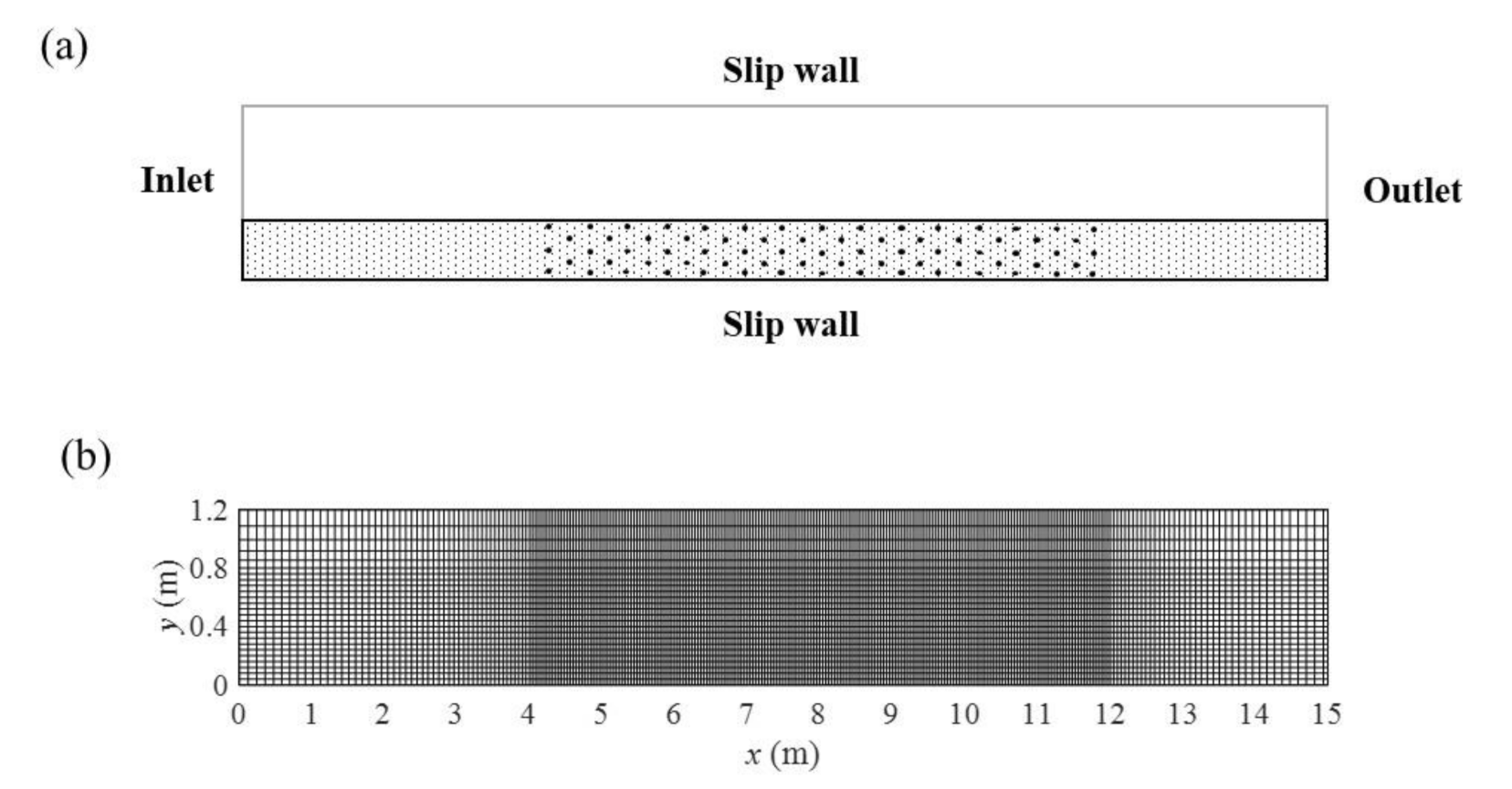
2.2. Numerical Model Setup

The simulated channel is three-dimensional flat domain and has 15 m length and 1.2 m width as Figure 1a, which is similar to the laboratory setting of White and Nepf [11,12]. The stream-wise, lateral, and vertical coordinates and velocities are x , u , y , v and z , w , respectively. The vegetated area is constructed with about 2400 cylinders of 0.6   cm diameter and 0.4 m height, which are distributed over one side of the channel. It consists of lots of rigid cylinders and they are spaced 6 and 4 cm apart from each other in x, y directions, respectively. Also, these cylinders are treated as impermeable wall, so they have no-slip condition and zero-gradient condition for velocity pressure boundary condition, respectively. These cylinders are distributed over one side of the channel. To be specific, the array of circular cylinders extends from x = 4 m to 12 m in stream-wise direction and from 0 m to 0.4 m width in lateral direction. This vegetated area condition corresponds to the case which has the volume fraction 0.045 in White and Nepf [12]. In other words, in the present setups for the numerical experiments, the ratio of the bottom area to the cylinder surface area is set to 0.015 . To acquire highly reliable results even inside of the vegetated area, the calculations are performed on grids consisting of up to 27 million cells. The range of grid sizes is 4 mm to 1.25 cm in x and y directions and 4 cm in z direction. Figure 1b illustrates the computational domain on the x-y plain which is reduced by 10 times smaller than real scale. As in Figure 1b, the mesh is much finer near the array of the cylinders than other areas. The grid sizes near the cylinders are 4 mm, 4 mm, 4 cm in x, y, z directions, respectively.
In this work, 7 cases are used to verify the coincidence with LCSs and particle trajectories, and to find out effects of vegetation and geometrical changes. Test case has similar geometry of the previous study by Luo et al. [32], and it is used to confirm the different dispersion pattern depending on the Stokes number. Cases 1 to 5 are composed of the compound channel geometry. In a natural channel, the mainstream is generally expected to be deeper than the vegetated area and so the present work used the fixed depth of the vegetated area for all cases and varies the depths in the mainstream. Case 1 has same depths of mainstream and vegetated area, and the mainstream depth is increasing by 0.2   m from case 1 to case 5. The depths of mainstream and vegetated area are represented by h m and h v , respectively, as shown in Figure 2a. The relative water depth is indicated as:
h r = h v / h m
Although the depths of the mainstream are various in each case, the discharges in all cases are fixed at a constant which is similar to the laboratory settings of White and Nepf [11,12]. Case 4-1 has the same geometry of case 4, but their discharges are different. The discharge in the case 4-1 is determined at a value that makes the velocity in the main channel similar to the case 1. The velocities are laterally uniform at the inlet and the pressure heads are laterally constant at the outlet, respectively. Most of the variables such as velocities and depths are spatiotemporally averaged to prevent confusion by fluctuations. The spatial average is taken over a characteristic horizontal area which is only occupied by fluid [11,12]. A temporally averaging period is 25 s which is slightly larger than the period of a wake which will be discussed later. The angle bracket and the overbar denote spatial and temporal averages, respectively. The approximate cross-section domain and the spatial averaged area, the characteristic horizontal area A f , are illustrated in Figure 2b. Table 1 summarizes the averaged variables for each simulation case.

2.3. Finite-Time Lyapunov Exponent (FTLE)

The LCS approach is a methodology that can capture the emergent patterns of flows and also can be used to understand the trapping mechanism of the particles without direct calculation for tracing them. The LCS have been used to describe the hydrodynamic structure of flows resulting from the numerical simulation [24,25,33] and the laboratory experiments [34,35]. When the LCSs are compared with sediment particle behaviors and trajectories, they are related to the transport and dispersion pattern of small particles [25].
One of popular ways to construct the LCS is using the finite-time Lyapunov exponents (FTLE) to find separatrix in a time-dependent system. Generally, the ridges of the FTLE are used as a measure of local chaos and one can estimate the spreading of fluid particles in a region of the flow during a finite time related to a distance from the initial points [36]. Therefore, the present study visualizes the structures of flows with the LCS method based on the FTLE. Note that we are following notations and equations for FTLE to Haller [23] and Shadden et al. [22].
Firstly, flow maps, f , indicate positions to describe the fluid motion:
f x 0 = x t ; t 0 , x 0
and it is based on the velocity fields:
x ˙ = u x , t
where x is the location vector, t is the time interval of [ t 0 , t 1 ] , and the subscript of 0 means the initial point. The trajectory of infinitesimal perturbation δ x is expressed δ x = f x 0 δ x t 0 since the higher-order term can be dropped. So, the size of the perturbation is:
δ x t = δ x t 0 , f x 0 T f x 0 δ x t 0
where ‖ ‖ denotes the inner product. In the above equation, the Cauchy–Green strain tensor f x 0 T f x 0 is a symmetric matrix to represent only the stretching by eigenvectors of it in a given flow. With those eigenvectors, the FTLE is defined as:
σ x 0 = 1 t 1 t 0 log λ max x 0
where λ max is the largest eigenvalue. In other words, the FTLE is interpreted as an average exponential growth of the largest stretching rate. Finally, the LCSs can be defined or represented by the ridges of the FTLE. They are called material lines and surfaces, and play as barriers through which no particle can pass [22].
A code for calculating FTLE used in the present work is the LCS MATLAB kit version 2.3 [37]. The tool kit consists of two main parts for calculation; one part firstly converts the original data file into a MATLAB data format and another part calculates the FTLE. The part for converting data was built again to reduce computational cost and time in this work, and the MATLAB kit calculates and constructs the LCS.

2.4. Particle Tracking Method

In order to validate the LCS analysis, the results from the LCS are compared to those from a conventional Lagrangian Particle Tracking (LPT) method. The present work is following the notations and equations of Vallier [38] to describe the motions and locations of particles in the LPT method. In this work, LPT method is solved by the code built in the OpenFOAM software. In a Lagrangian frame, the position vector of particles x p is calculated with the following equation:
d x p d t = u p
The momentum of particles is described by particle momentum equation as:
m p d u p d t = F
where u p is the velocity of particles, m p is the mass of particles, and F is the force acting on particles. The particles with three different densities are tested to compare with the LCS for the validation of tracking trajectories. The details of particles are summarized in Table 2.
The properties of particle behavior can be represented by the Stokes number (St). It is a dimensionless number representing the ratio of the characteristic time of particle to that of flow. It is defined as [39]:
S t = t p t f
where t p and t f are the particle characteristic time and flow characteristic time, respectively. They are obtained by:
t p = ρ p D p 2 18 μ   and   t f = D U
in which D is the diameter of a cylinder, U is the free stream velocity which is selected as 0.05   m / s in most cases, and ρ p and D ρ are the density and diameter of particle, respectively.
The comparison of the LCS results to those of LPT are done by the simulation in a two-dimensional domain with a length of 1.4   m and a width of 0.8   m . This dimension of the domain is chosen to avoid the effect of the boundaries on the wake development [40]. In the domain, a single circular cylinder D of 0.04   m is deployed, and particles are released at the upstream of that cylinder.

3. Results and Discussion

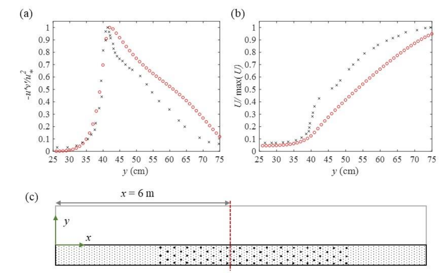
3.1. Validation of the LCS and CFD

The first validation experiment using test case in Table 1 is to confirm the LCS to track the particle trajectories. Luo et al. [32] conducted a similar experiment and verified the different dispersion pattern depending on the Stokes number. In this work, 30 particles are injected every 0.5 s and a total of 600 particles are released for each case. Figure 3 shows the trajectories of particles with the different Stokes numbers, 0.005, 0.1 and 0.5 along the LCS line. When St = 0.005 (Figure 3a), the particles follow the LCS lines closely and that line shows circulations reconstructing the vortex structures at an almost identical location to the particle trajectory. When the Stokes number increases to 0.1 (Figure 3b), the particles still flow along the LCS lines very similar to Figure 3a, even though the particle concentration near the core of the vortex becomes lower than the case of St = 0.005. It means that inertia affects more significantly when curvature changes fast and angular momentum is strong. As the Stokes number becomes larger to be 0.5, the particles flow in a distance slightly away from the LCS lines as in Figure 3c. In this last case, the trajectories of particles are quite different from the LCS structures. Besides, there are no particles in the vortex since in this case, the particle response time to the fluid flow must be much higher than the other cases with the smaller Stokes numbers. Therefore, as the Stokes number is getting smaller, the trajectories of particles seem to be reasonably reconstructed by the LCS line.
The second validation experiment is to check that our results are in line with laboratory measurements in White and Nepf [11,12]. The momentum exchange and normalized stream-wise velocity were acquired at x = 6 m away from the inlet, and the part where vegetation and the main channel met was set to y = 0 (Figure 4c). The objective of the present work is to investigate the possibility of the LCS to analyzing the flow structures, so we have not sought to verify in detail the realism of the simulation results beyond what these prior studies have done. The normalized Reynolds stress and stream-wise velocity obtained by White and Nepf [11,12] are compared to the present numerical simulations, respectively, as shown in Figure 4. The normalized Reynolds stress of simulation results decreases as getting far from the vegetated area less than the laboratory experiments when x is larger than zero. Moreover, the profiles of the stream-wise velocity of the laboratory experiments are slightly faster than the numerical simulation. However, both results had a similar tendency, so we conclude that the proposed numerical simulation method can reproduce the overall tendency of flow properties and the mechanisms of material transport within a reasonable and allowable range. The discrepancy between the results from the laboratory and numerical experiments is suspected due to the natural limitation of the presently utilized RANS model.

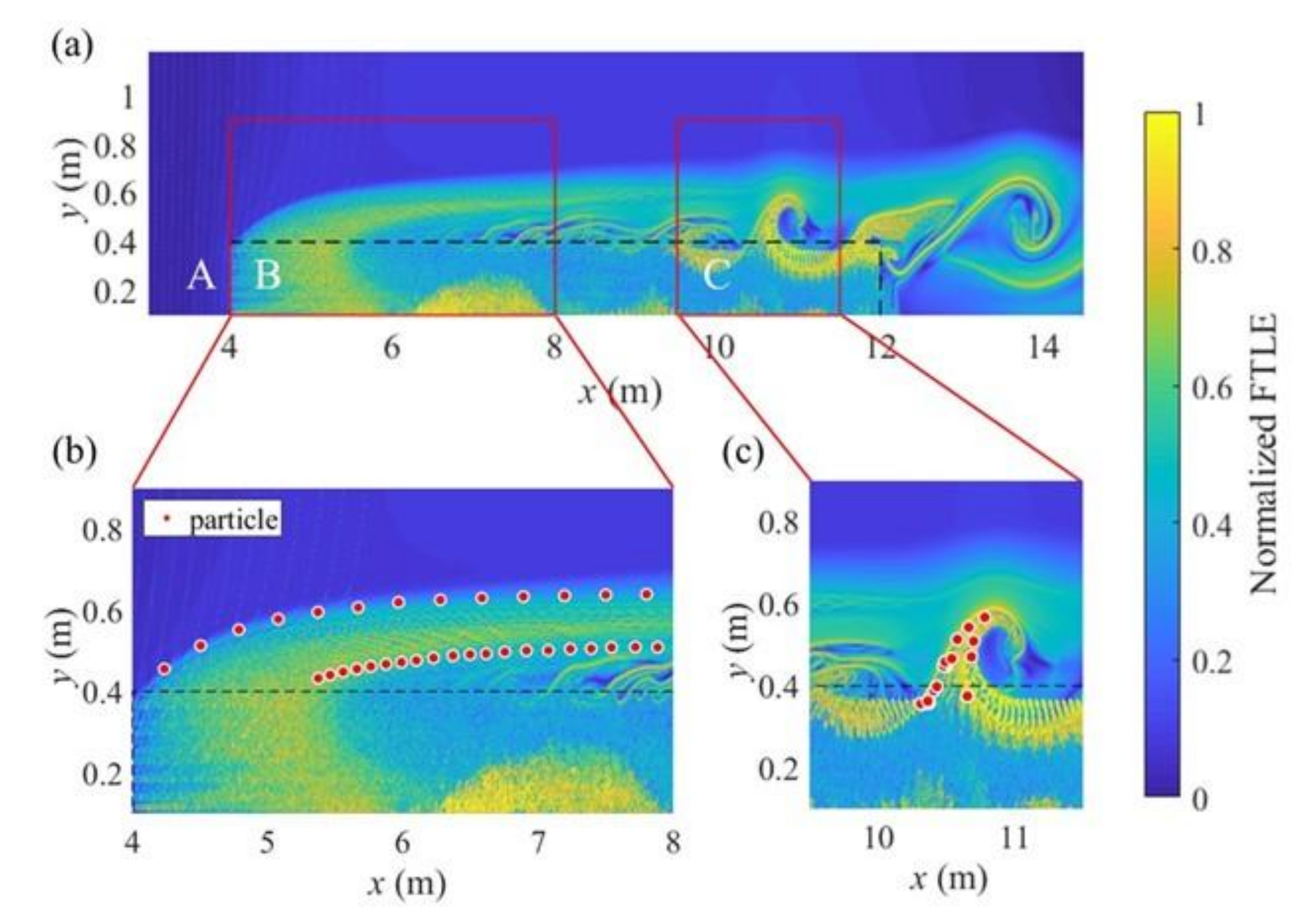
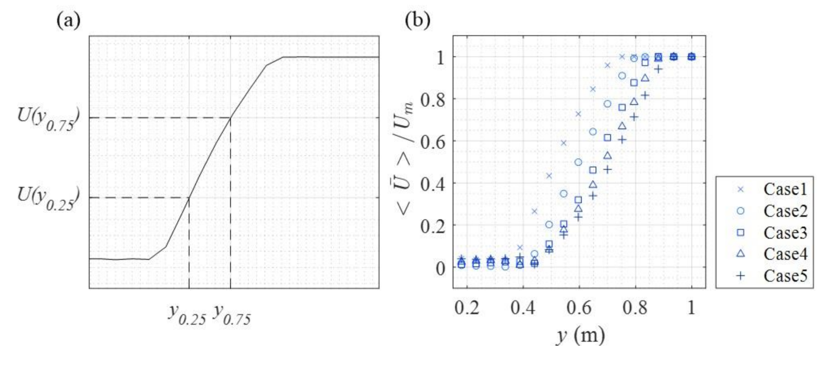
3.2. Simulation Results and Discussion

White and Nepf [11,12] observed vortex structures in the strongly sheared regions between mainstream and vegetated areas after releasing sediments of particles instantaneously. Such vortex structures often occur in a vertical direction when the flow is stratified and has different velocities at each layer and also as in the present case, flows with the steep lateral velocity gradients bring those vortices as like as in a region where two streams merge. While the vortices in the vertically layered flows are constrained by free water surface or vertically extended stratification, laterally separated flows seem to have a much larger size of vortex since there is no serious constraint except the channel width. Therefore, this large-scale recirculation near the interface between the mainstream and vegetated seems to play a major role in exchanging momentum and materials between areas.
The quantitative visualization of a vortex structure in the simulation results is conducted by the LCS method. The instantaneous FTLE field of case 1 is constructed with the velocity fields and this FTLE presents not only the structures of the vortex but also its downstream migration, which could be a crucial component in determining interfacial boundaries between main and vegetation affecting areas.
The FTLEs are normalized by their maxima as Figure 5. Figure 5b,c also compare the FTLE to particle trajectories by LPT with the Stokes number of 0.005 to avoid the significant effects of the inertia. The particles are injected as three groups: the first group of particles is placed at the zone A which has relatively lower FTLE, while the second and third particle groups are released in the zone B and C of relatively higher FTLE, respectively (Figure 5a). The particles in the first group flow downstream along the boundary of the FTLE, and stay within the mainstream zone but away from the vegetated zone (Figure 5b). The particles of the second group, placed inside of the vegetated area, are spit out from the vegetated area and flow along the yellow line boundary or ridge of an FTLE toward downstream (Figure 5b). The particles of third group, released far downstream, flow initially following the left limb of the wavy vortex getting away from the vegetated area but move back into the vegetated area following the right limb of the wavy vortex (Figure 5c). Since the LCSs and particle trajectories are pretty much identical, the flow topology visualized by LCS can predict movement well.
The geometrical effects on flow structures are investigated by varying the depths of the mainstream. The cases of 1, 2, and 4 have different depth ratios, H r (Table 1). When the depths of mainstream and vegetated area are same (i.e., h r is 1), a strong FTLE value appears close to the interface between mainstream and vegetated area, showing sharp-edged vortex structures than other cases. The radii of the vortices formed near the interfacial layer are getting larger as the vortex migrates downstream.
When h r   becomes smaller to 0.67 (i.e., case 2), there is no significant difference compared with h r = 1 and the width of FTLE gradually increases slightly more than the case of h r = 1, toward the downstream. The size of the vortex seems to get larger since the increases of depth decrease both flow velocities in the mainstream and the vegetated area simultaneously. However, larger gradient between those two areas results in increasing mixing layer thickness between mainstream and vegetated area. The phenomenon of larger mixing layer thickness and vortex size seems to be similar to what is found in the laminar flow with a wider boundary layer than that of turbulent flow. It is probably due to lower transport or supply of momentum from the mainstream to the area where the energy is being depleted. It will be discussed later, but we can confirm by the fact that the shear stress in the mixing layer decreases as the velocity gradient decreases (Figure 8). When h r is 0.4, the FTLE moves further away from the vegetated area (Figure 6c). In this case, it is hard to form the vortex differently from the other cases of the higher h r .
To investigate only the geometrical effects or depth variations, excluding the effects of the velocity gradient, the case 4-1 is set to the velocity distribution similar to the case 4 and the lateral gradient at the near-surface similar to the case 1 (Table 1). The widths of FTLEs in case 4 and case 4-1 are similar to each other except subtle differences of higher FTLE at the edge of the interfacial layer in case 4-1 (Figure 6c,d). Additionally, the vortex forms more apparently in case 4-1 than that of case 4. When comparing the case 4-1 to the case 1, larger vortices and thicker interfacial mixing layers are found in the case 4-1. Deeper depth in the case of 4-1 may allow the vortex to develop with smaller depth constriction and let it grow further.
To represent the mixing intensity, mean stream-wise velocities within the vegetated field and the mainstream ( U v and U m , respectively) are compared with each other which are the mean stream-wise velocities within the vegetated field and the mainstream, respectively. Both velocities are averaged for 25 s which is similar to the wake period or time for a cycle. The difference between U v and U m causes the presence of mixing. Following to the methods suggested in Van Prooijen et al. [16], the width of the mixing layer is determined by estimating the distance between the positions of y 0.25 and y 0.75 , of which the subscript 0.25 and 0.75 indicate the locations having 25% and 75% of the velocity differences. It can be obtained as:
U y 0.25 = U v + 0.25 U m U v ,   U ( y 0.75 = U v + 0.75 U m U v
where the mixing layer width is defined:
δ = 2 y 0.75 y 0.25 .
The two positions, y 0.25 and y 0.75 , which determine the mixing layer are shown in Figure 7a for clarity.
As shown in Table 3, the averaged velocities decrease as the mainstream depth increases. This is somewhat expected since the discharge of water is constant. The velocity difference between the main and vegetated channel is getting smaller as the depth ratio h r decreases as described above. To compare all cases having various mean velocities, the lateral velocities of each case are normalized by the mean stream-wise velocity of each case (Figure 7b). The mean velocities are measured at x = 8 m, which is the mid-point of the vegetated area. Moreover, the mean velocity was spatial and averaged the depth and space between cylinders.
In case 1, the velocity remarkably changes near the vegetated region, and as the depth of the mainstream increases, the inflection points of velocity gradient get away from the vegetated area. The changes of the gradients and those maximum magnitudes may significantly affect shear stress which quantifies the momentum exchanges between the areas.
The amount of momentum exchange between the mainstream and vegetated zone is obtained by:
T x y ρ u v ¯
where u and v are the fluctuating stream-wise and lateral velocities, respectively.
The amounts of momentum exchange at x = 9   m in each case are illustrated in Figure 8a. As h r decreases, the portions of positive momentum exchange value become wider and move towards the mainstream. Similar trends were observed in the analysis with the normalized FTLE, where the width of FTLE is getting wider as h r is getting smaller (Figure 6). Additionally, the point of maximum momentum exchange, i.e., the location where the largest shear stress occurs, moves toward the mainstream. So, the mixing zone moves from the region near the vegetated area to the mainstream. The momentum exchange at different positions in case 1 is shown in Figure 8b. As we can expect, the maximum value and thickness of momentum exchange is getting larger along the flow. As can be seen in Figure 6a, the flow is complicated as a vortex is generated near the vegetation interface. Therefore, there are two local maximums at x = 12 m unlike other positions.

4. Conclusions

The present work investigated the flow structure near the vegetation in a channel, by applying the LCS analysis based on the FTLE calculation. The results confirmed that the LCS method is a suitable tool to evaluate material transport even in a channel with a complex cross-section and vegetation. The FTLE visualizes well the existence of interfacial layers (i.e., boundaries between the mainstream and vegetated area) and the migration of vortices (i.e., the sub-structures of the interfacial layer). Comparison of the particle trajectories to the ridge of the FTLE illustrates that the particles follow closely to the ridge of FTLE along with the contours of the vortex, flowing out from the vegetated area to the main channel. This method must be helpful to overcome the limitations of the particle tracking method, in which costs are computationally very expensive and take a long time for simulation.
There are several new findings with the LCS analysis for the flow field in the vegetated compound channels. The width of FTLE becomes wider as h r decreases. Relatively higher values of FTLE are located far from the vegetated area, which has not been reported in previous studies. The variations of depth also affect the formation of the vortex. The radius of the vortex becomes larger as h r decreases. The results show that it is hard to form the vortex in the condition with the smallest h r . As the velocity difference is getting smaller, the maximum amount of momentum exchange decreases. However, the momentum needs to be supplied from a place far away.
The present work makes progress in understanding the complicated interactions between the cylinders and also in confirming the effect of depth difference. However, it should be noted that the free surface is not included in this study which warrants further research in the future. It might allow the slope to be between the main and vegetated channel, and extra interactions could be invoked. In addition, the LCS method needs to be extended to a three-dimensional analysis, which can help to visualize the vortex structure and investigate the material transport through interfacial surfaces.

Author Contributions

Funding acquisition, J.H.H.; Software, S.C.; Supervision, J.H.H.; Validation, S.C.; Writing—original draft, S.C.; Writing—review & editing, S.C. and J.H.H. All authors have read and agreed to the published version of the manuscript.

Funding

This research was funded by the project entitled “Development of Advanced Science and Technology for Marine Environmental Impact Assessment” (grant number 20210427) funded by the Ministry of Oceans and Fisheries of Korea (MOF), “Chemical Accident Response R&D program” (No. 1485017731) funded by Korea Ministry of Environment (MOE) and administratively supported by the Institute of Engineering Research at Seoul National University.

Institutional Review Board Statement

Not applicable.

Informed Consent Statement

Not applicable.

Data Availability Statement

The data presented in this study are available on request from the corresponding author.

Conflicts of Interest

The authors declare no conflict of interest.

References

  1. Liu, P.L.F.; Chang, C.W.; Mei, C.C.; Lomonaco, P.; Martin, F.L.; Maza, M. Periodic water waves through an aquatic forest. Coast. Eng. 2015, 96, 100–117. [Google Scholar] [CrossRef]
  2. Kobayashi, N.; Raichle, A.W.; Asano, T. Wave attenuation by vegetation. J. Waterw. Port Coast. Ocean Eng. 1993, 119, 30–48. [Google Scholar] [CrossRef]
  3. Brunone, B.; Tomasicchio, G.R. Wave kinematics at steep slopes: Second-order model. J. Waterw. Port Coast. Ocean Eng. 1997, 123, 223–232. [Google Scholar] [CrossRef]
  4. Grove, A.S.; Shair, F.H.; Petersen, E.E. An experimental investigation of the steady separated flow past a circular cylinder. J. Fluid Mech. 1964, 19, 60–80. [Google Scholar] [CrossRef]
  5. Anderson, E.A.; Szewczyk, A.A. Effects of a splitter plate on the near wake of a circular cylinder in 2 and 3-dimensional flow configurations. Exp. Fluids 1997, 23, 161–174. [Google Scholar] [CrossRef]
  6. Brandon, D.J.; Aggarwal, S.K. A numerical investigation of particle deposition on a square cylinder placed in a channel flow. Aerosol Sci. Technol. 2001, 34, 340–352. [Google Scholar] [CrossRef]
  7. Vu, H.C.; Ahn, J.; Hwang, J.H. Numerical simulation of flow past two circular cylinders in tandem and side-by-side arrangement at low Reynolds numbers. KSCE J. Civ. Eng. 2016, 20, 1594–1604. [Google Scholar] [CrossRef]
  8. Zinke, P. Application of Porous Media Approach for Vegetation Flow Resistance; CRC Press: Boca Raton, FL, USA, 2012; pp. 301–307. [Google Scholar]
  9. Brito, M.; Fernandes, J.; Leal, J.B. Porous media approach for RANS simulation of compound open-channel flows with submerged vegetated floodplains. Environ. Fluid Mech. 2016, 16, 1247–1266. [Google Scholar] [CrossRef] [Green Version]
  10. Bennett, S.J.; Pirim, T.; Barkdoll, B.D. Using simulated emergent vegetation to alter stream flow direction within a straight experimental channel. Geomorphology 2002, 44, 115–126. [Google Scholar] [CrossRef]
  11. White, B.L.; Nepf, H.M. Shear instability and coherent structures in shallow flow adjacent to a porous layer. J. Fluid Mech. 2007, 593, 1–32. [Google Scholar] [CrossRef]
  12. White, B.L.; Nepf, H.M. A vortex-based model of velocity and shear stress in a partially vegetated shallow channel. Water Resour. Res. 2008, 44. [Google Scholar] [CrossRef]
  13. Zhang, J.T.; Su, X.H. Numerical model for flow motion with vegetation. J. Hydrodyn. 2008, 20, 172–178. [Google Scholar] [CrossRef]
  14. Zong, L.; Nepf, H. Flow and deposition in and around a finite patch of vegetation. Geomorphology 2010, 116, 363–372. [Google Scholar] [CrossRef]
  15. Park, H.; Hwang, J.H. Quantification of vegetation arrangement and its effects on longitudinal dispersion in a channel. Water Resour. Res. 2019, 55, 4488–4498. [Google Scholar] [CrossRef] [Green Version]
  16. Truong, S.H.; Uijttewaal, W.S.J. Transverse momentum exchange induced by large coherent structures in a vegetated compound channel. Water Resour. Res. 2019, 55, 589–612. [Google Scholar] [CrossRef]
  17. Tominaga, A.; Nezu, I. Turbulent structure in compound open-channel flows. J. Hydraul. Eng. 1991, 117, 21–41. [Google Scholar] [CrossRef]
  18. Sofialidis, D.; Prinos, P. Compound open-channel flow modeling with nonlinear low-Reynolds k-ϵ models. J. Hydraul. Eng. 1998, 124, 253–262. [Google Scholar] [CrossRef]
  19. Van Prooijen, B.C.; Battjes, J.A.; Uijttewaal, W.S. Momentum exchange in straight uniform compound channel flow. J. Hydraul. Eng. 2005, 131, 175–183. [Google Scholar] [CrossRef]
  20. Salamon, P.; Fernàndez-Garcia, D.; Gómez-Hernández, J.J. A review and numerical assessment of the random walk particle tracking method. J. Contam. Hydrol. 2006, 7, 277–305. [Google Scholar] [CrossRef]
  21. Zhang, P.F.; Wang, J.J.; Huang, L.X. Numerical simulation of flow around cylinder with an upstream rod in tandem at low Reynolds numbers. Appl. Ocean Res. 2006, 28, 183–192. [Google Scholar] [CrossRef]
  22. Shadden, S.C.; Lekien, F.; Marsden, J.E. Definition and properties of Lagrangian coherent structures from finite-time Lyapunov exponents in two-dimensional aperiodic flows. Phys. D Nonlinear Phenom. 2005, 212, 271–304. [Google Scholar] [CrossRef]
  23. Haller, G. Lagrangian coherent structures. Annu. Rev. Fluid Mech. 2015, 47, 137–162. [Google Scholar] [CrossRef] [Green Version]
  24. Son, Y.B.; Kim, Y.H.; Choi, B.-J.; Park, Y.-G. Lagrangian coherent structures and the dispersion of green algal bloom in the Yellow and East China Sea. J. Coast. Res. 2015, 75, 1237–2141. [Google Scholar] [CrossRef]
  25. Ku, H.; Hwang, J.H. The Lagrangian Coherent Structure and the Sediment Particle Behavior in the Lock Exchange Stratified Flows. J. Coast. Res. 2018, 85, 976–980. [Google Scholar] [CrossRef]
  26. Fischer-Antze, T.; Stoesser, T.; Bates, P.; Olsen, N.R.B. 3D numerical modelling of open-channel flow with submerged vegetation. J. Hydraul. Res. 2001, 39, 303–310. [Google Scholar] [CrossRef]
  27. Neary, V.S. Numerical solution of fully developed flow with vegetative resistance. J. Eng. Mech. 2003, 129, 558–563. [Google Scholar] [CrossRef]
  28. Woelke, M. Eddy Viscosity Turbulence Models employed by Computational Fluid Dynamic. Prace Inst. Lotnictwa 2007, 4, 92–113. [Google Scholar]
  29. Menter, F.R.; Kuntz, M.; Langtry, R. Ten years of industrial experience with the SST turbulence model. Turbul. Heat Mass Transf. 2003, 4, 625–632. [Google Scholar]
  30. Open, C.F.D. OpenFOAM user guide. OpenFOAM Found. 2011, 2, 103. [Google Scholar]
  31. López, A.; Nicholls, W.; Stickland, M.T.; Dempster, W.M. CFD study of jet impingement test erosion using Ansys Fluent® and OpenFoam®. Comput. Phys. Commun. 2015, 197, 88–95. [Google Scholar] [CrossRef] [Green Version]
  32. Luo, K.; Fan, J.; Jin, H.; Cen, K. LES of the turbulent coherent structures and particle dispersion in the gas–solid wake flows. Powder Technol. 2004, 147, 49–58. [Google Scholar] [CrossRef]
  33. Green, M.A.; Rowley, C.W.; Haller, G. Detection of Lagrangian coherent structures in three-dimensional turbulence. J. Fluid Mech. 2007, 572, 111–120. [Google Scholar] [CrossRef] [Green Version]
  34. Voth, G.A.; Haller, G.; Gollub, J.P. Experimental measurements of stretching fields in fluid mixing. Phys. Rev. Lett. 2002, 88, 254501. [Google Scholar] [CrossRef] [PubMed] [Green Version]
  35. Mathur, M.; Haller, G.; Peacock, T.; Ruppert-Felsot, J.E.; Swinney, H.L. Uncovering the Lagrangian skeleton of turbulence. Phys. Rev. Lett. 2007, 98, 144502. [Google Scholar] [CrossRef]
  36. Rempel, E.L.; Chian, A.C.; Brandenburg, A. Lagrangian chaos in an ABC-forced nonlinear dynamo. Phys. Scr. 2012, 86, 018405. [Google Scholar] [CrossRef] [Green Version]
  37. John, O.D. LCS MATLAB Kit Version 2.3; California Institute of Technology, Pasadena, California, USA. Available online: http://dabirilab.com/software/. (accessed on 26 March 2016).
  38. Vallier, A. Tutorial icolagrangianfoam/solidparticle. In Peer Reviewed Tutorial, Hakan Nilsson, CFD with OpenSource Software; Chalmers University of Technology: Goteborg, Sweden, 2009. [Google Scholar]
  39. Lau, T.C.; Nathan, G.J. The effect of Stokes number on particle velocity and concentration distributions in a well-characterised, turbulent, co-flowing two-phase jet. J. Fluid Mech. 2016, 809, 72–110. [Google Scholar] [CrossRef] [Green Version]
  40. Mahir, N.; Altaç, Z. Numerical investigation of convective heat transfer in unsteady flow past two cylinders in tandem arrangements. Int. J. Heat Fluid Flow 2008, 29, 1309–1318. [Google Scholar] [CrossRef]
Figure 1. (a) Numerical simulation domain and boundary condition; (b) 10 times grid size computational domain in x-y plain for compound channel.
Water 14 00406 g001
Figure 2. (a) The computational domain cross-section; (b) Spatial averaged area occupied only fluid in top view with the characteristic horizontal area, A f .
Water 14 00406 g002
Figure 3. The normalized FTLE and instantaneous positions of particles (red dots): (a) St = 0.005; (b) St = 0.1; (c) St = 0.5; cylinder position (blue circle).
Water 14 00406 g003
Figure 4. The normalized (a) Reynolds stress and (b) stream-wise velocity: White and Nepf [11,12] (crosses) and the simulation results (circle); (c) Data collected position.
Water 14 00406 g004
Figure 5. (a) Normalized FTLE in horizontal plain for case 1 with cylinder zone (black dash line) and (b,c) with particles (red dots).
Water 14 00406 g005
Figure 6. Normalized FTLE in horizontal plain, the vegetated area enclosed by the black dash line: (a) Case 1; (b) Case 2; (c) Case 4; (d) Case 4-1.
Water 14 00406 g006
Figure 7. (a) Definition sketch for y 0.25 and y 0.75 and (b) Normalized stream-wise velocity: ×: case 1; ○: case 2; □: case 3; △: case 4; +: case 5.
Water 14 00406 g007
Figure 8. (a) Momentum exchanges in each case at x = 9   m ; (b) Momentum exchanges of case 1 at x = 4, 6, 8, 10, 12 m.
Water 14 00406 g008
Table 1. Variables and results for each case.
Test CaseCase 1Case 2Case 3Case 4Case 4-1Case 5
Mean   Inlet   Velocity   ( m / s )0.0500.1030.0770.0620.0510.1300.044
Domain Size ( x × y × z ,   m 3 ) 1.4 × 0.8 × 0.2 15 × 1.2 × 0.4 15 × 1.2 × 0.4 15 × 1.2 × 0.4 15 × 1.2 × 0.4 15 × 1.2 × 0.4 15 × 1.2 × 0.4
Cylinder   Diameter   ( cm )4.00.60.60.60.60.60.6
h r 1.001.000.670.500.400.400.33
Table 2. Three types of particle parameter: diameter, density, and Stokes number.
Diameter   ( D p ) Density   ( ρ p ) Stokes   Number   ( S t )
0.0028   m 90   kg / m 3 0.005
0.0028   m 1800   kg / m 3 0.1
0.0028   m 9000   kg / m 3 0.5
Table 3. Parameters and results for each case.
Case 1Case 2Case 3Case 4Case 5
U m   ( cm / s ) 16.14   10.79   8.01   6.29   5.20  
U v cm / s 2.55   1.76 1.36   1.14   1.00  
y 0.25 cm 44.0   54.4   59.6   64.8   64.8  
y 0.75 cm 59.6   70.0   75.2   79.4   79.4  
δ cm 31.2   31.2   31.2   29.2   29.2  
Publisher’s Note: MDPI stays neutral with regard to jurisdictional claims in published maps and institutional affiliations.

