Abstract
In South Korea, flood damage mainly occurs around rivers; thus, it is necessary to determine the optimal design frequency for river basins to prevent flood damage. However, there are not enough studies showing the effect of climate change on hydrologic design frequency. Therefore, to estimate the optimal design frequency according to future climate change scenarios, this study examined urban flooding area and extreme rainfall frequency that can change in the future. After estimating the optimal design frequency, hydrological risks of 413 local river basins were evaluated according to Representative Concentration Pathway (RCP) scenarios 4.5 and 8.5 after regenerating daily rainfalls from the HadGEM2-ES model into hourly rainfalls using the Poisson cluster. For the RCP 4.5, hydrological risks increased relative to the established design frequency by 3.13% on average. For the RCP 8.5, hydrological risks increased by 2.80% on average. The hydrological risks increased by 4.58% in the P2(2040–2069) period for the RCP 4.5, and by 4.39% in the P1 (2021–2039) period for the RCP 8.5. These results suggest that the hydrologic design frequency in the future will likely decrease, and the safety of river basins will also decrease.
1. Introduction
In South Korea, approximately 90% of damage caused by natural disasters are related to climate change; among them, more than 80% result from heavy rains, typhoons, and storms [1]. The total damage from storms over the last decade including heavy rain, heavy snow, and typhoon and floods was KRW 3,397,332 million, which is 96.6% of the total disaster damage [2]. Storms and floods account for a larger proportion of damage caused by natural disasters each year; it is mainly due to the increase in impervious areas due to the continuous development of land and the increase in localized torrential rain due to climate change. Spatio-temporal variations of precipitation are continuously increasing in South Korea. Annual precipitation has large variations ranging from 754 mm at the minimum to 1756 mm at the maximum, and the frequency of extreme floods is increasing. Precipitation concentrated the flood season (i.e., from June to September that accounts for 68% of annual precipitation, precipitation greatly varied by region (1729 mm at the maximum on Jeju Island, 1240 mm at the minimum for Geum River), and mountainous terrain that covers 65% of the national land and makes steep slopes of most rivers cause rapidly increased flood runoff. Due to such precipitation and topographical characteristics, South Korea is highly vulnerable to floods, and this is further aggravated by climate change. Therefore, proper maintenance of rivers can prevent disasters caused by floods, and the optimal design frequency must be ascertained.
In South Korea, hydrologic design frequency is determined by considering the importance of a river (‘A’ for critical areas of national rivers, ‘B’ for national rivers, and ‘C’ for local rivers) and regional characteristics (i.e., urban, agricultural, and mountainous areas). These criteria cannot accurately reflect topographical and water control characteristics since they have a large scope of applications and there are no specific evaluation standards. Recent studies have attempted to determine hydrologic design frequency based on the characteristics of rivers as well as the status of protected lowlands. Chungcheongnam-do [3] has suggested a practical method of deciding the optimal design frequency of local rivers based on six evaluation factors: inland conditions, watershed area, river length, river width, river channel slope, and river stream order. Chungcheongnam-do [3] also calculated weights for six evaluation factors using the analytic hierarchy process (AHP) and determined the final design frequency considering the derived potential flood damage (PFD) for each region. Although experts participated in the question survey during the AHP for determining weights of the evaluation factors, the results depend on their subjective answers. Moreover, many studies identified climate change as the major cause for the occurrence and the increase of heavy storms and floods but there were no factors reflecting the impact of climate change in the decision-making process of design frequency. The main objective of this study is to propose an innovative method for determining the optimal design frequency by improving the methodology of Chungcheongnam-do [3], to provide engineering objectivity and include the impacts of climate change.
Recently, objective probabilistic and statistical techniques have been used to exclude subjective factors from the weight calculation process of evaluation factors. Such objective weight calculation methods are often used when evaluating vulnerability and risk. The most frequently used objective weight calculation methods include the arithmetic mean and the weighted mean. However, these methods are hard to accurately explain the impacts and contributions of various evaluation factors. Lee et al. [4] used arithmetic mean, weighted mean, and principal component analysis to determine flooding risk considering the flood control ability of each region. The arithmetic mean method had problems giving the same weight to factors possessing different characteristics, while the weighted mean method caused a multicollinearity problem. To solve these problems, the entropy method, principal component analysis (PCA), and Bayesian network method have been used. Chen et al. [5] calculated the flood disaster index that represents the risk of flooded areas by applying the entropy weight method. Lee et al. [6] evaluated the flood risks of urban watersheds by applying the PROMETHEE method (a multi-criteria decision-making technique) and the entropy method after classifying evaluation factors such as rainfall, runoff, and regional factors. Joo et al. [7] determined the water control investment priorities using an integrated index for flood risk assessment and the net present value for 28 municipalities in Chungcheong-do. They used integrated weights by combining the AHP, the constant sum scale, and the entropy method. In this way, efforts are being made to calculate objective weights through various methods, and appropriate methods can be applied according to the research objectives and data characteristics.
Regarding to impact of climate change on flood risk, the Ministry of the Interior and Safety [8] provided guidelines to enhance disaster prevention standards for disaster prevention facilities after quantitatively analyzing the effect of climate change on the meteorological factors including heavy rainfall causing disasters considering Representative Concentration Pathway (RCP) scenarios. Various studies demonstrated that the 100-year rainfall increased by 80% or higher according to the RCP 8.5 [8], the volume of a 100-year flood would increase by 10–24% in the future [9], and the 7-day annual maximum flow rate would increase by approximately 39% due to climate change [10]. In addition, many studies have analyzed the increased rates of rainfall and flood volume in study areas influenced by climate change [11,12,13,14]. Furthermore, some researchers have analyzed future risks by applying various climate change scenarios; the risk would increase by 14.1–18.3% for a 50-year flood when a future climate change scenario was applied [15], and the flood risk would increase by 19.3% compared to the present for a 100-year flood of the RCP 8.5 climate change scenario of the future [16]. Lee et al. [17] calculated future flood risk according to the design flood volume using a machine learning technique and showed that the risk increased by 8.7% for a 100-year flood in the RCP 8.5 scenario.
In this study, the hourly rainfalls were generated according to the RCP scenarios to investigate the change of design frequency due to climate change, and the weights of evaluation factors were calculated through Bayesian inference to determine the optimal design frequency for local rivers, resolving the practical issues of AHP. In addition, changes in the hydrologic design frequency and hydrological risks were then evaluated for future periods: P1 (Period 1: 2021–2039), P2 (Period 2: 2040–2069), P3 (Period 3: 2070–2099), and TP (Total period: 2021–2099).
2. Theoretical Background
2.1. Bayesian Inference
Statistical inferences refer to the process of drawing certain conclusions for parameters () from given observed data. Bayesian inference is recently known to be efficient to estimate parameters and to quantify their uncertainty because it updates parameters using the newly obtained samples or observations. Bayesian inference estimates the posterior distribution using the likelihood function and the prior distribution for the parameters. In general, when an observation data y, the likelihood function and prior distribution are given, the conditional probability of the unknown , posterior distribution , can be calculated as:
where is the likelihood function of , is the prior distribution of , and is the marginal distribution of y.
2.2. Poisson Cluster Rainfall Generation Model
Poisson cluster rainfall generation models are widely used to generate rainfall time series of daily or shorter time units. The models are classified into Bartlett–Lewis (BL) model and Neyman–Scott (NS) model according to the process to generalize the Rectangular Pulse (RP) model. Among them, the Bartlett–Lewis Rectangular Pulse (BLRP) model follows the Poisson cluster process, in which rain events are expressed by a cluster of cells that follow a Poisson distribution and have an RP with a certain intensity [18]. In addition, each cell is expressed by a cell length and rainfall intensity of a cell that exhibits exponential and gamma distributions. The initial BLRP model, which was conceptualized by Rodriguez-Iturbe et al. [18], has five parameters (, , , , ) to express the cell characteristics of a rainfall event. The arrival time of the rainfall cell follows a Poisson distribution with as a parameter, and the duration and rainfall intensity are determined by an exponential distribution with and . The arrival time of a rain event follows a Poisson distribution with , and the length of a rain event is determined by an exponential distribution with . and are converted to dimensionless values by and , respectively [18].
However, the percentage of zero rain period (zero depth period) of the rainfall time series simulated for various time ranges can sometimes fail to accurately reproduce the statistics of the observed time series. Therefore, the Modified Bartlett–Lewis Rectangular Pulse (MBLRP) model was developed by adding one parameter and changing the parameter representing the duration of a rain event to a gamma distribution. In the MBLRP model, the length of the rainfall cell is not obtained from an exponential distribution with , but from a gamma distribution with the shape factor and the scale factor . In other words, is replaced with and . A simulation time series is generated by six parameters (, , , , , ).
The statistics for estimating parameters are the mean of rainfall, the variance of rainfall, autocovariance, and the percentage of zero rain period.
The mean rainfall is expressed as:
where is the average of the number of rainfall cells per rain event, and it is expressed as ; c is the number of rainfall cells per rain event, and T is the time per duration.
The variance of rainfall is expressed as:
Autocovariance is expressed as:
where is the delay time, and and are expressed as and [19].
The percentage of zero rain period is expressed as:
where , , and are expressed as , , and [19].
2.3. Performance Measures of Poisson Cluster Rainfall Generation Model
To evaluate the applicability of the generated hourly rainfalls, the hourly rainfall data generated by the Poisson cluster model were aggregated again to daily rainfalls and then compared with those from the climate change scenarios. The performance was evaluated using the root mean squared error (RMSE), the normalized root mean squared error (NRMSE), and the root mean squared log error (RMSLE). For all three performance indicators, a value closer to zero (%) means a smaller difference between the measured and predicted values, as expressed in Equations (6)–(8):
where is the daily rainfall of the climate change scenario; is the daily rainfalls re-aggregated from the generated hour rainfalls by the Poisson cluster model; and and are the maximum and minimum values.
3. Estimation of Optimal Design Frequency for Local Rivers
3.1. Study Area
We proposed the optimal design frequency calculation method using Bayesian inference and applied it to 413 local rivers in Chungcheongnam-do. Figure 1 shows the locations of Chungcheongnam-do. The total area of Chungcheongnam-do is 8204 km2, accounting for approximately 8.6% of the total area of South Korea, 99,617 km2.
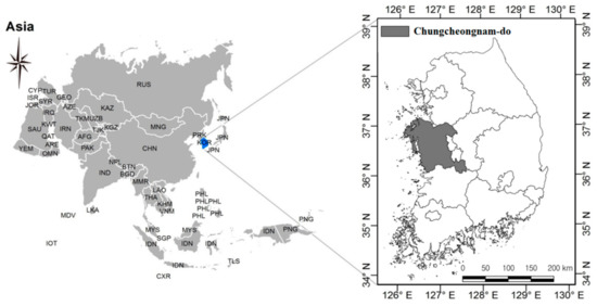
Figure 1.
Map of the study area.
The determination of hydrologic design frequency is directly related to the efficiency and economic feasibility of the target project when establishing a river master plan. The setting of the design frequency is crucial when considering ripple effects such as an increase in incorporated land due to the retreat of the rear slope, besides simply setting a high embankment height.
The design frequency of local rivers of Chungcheongnam-do is determined through evaluation factors in accordance with the “Chungcheongnam-do local rivers optimal design frequency decision method” [3]. There are seven evaluation factors of Chungcheongnam-do [3] including urban flooding area, watershed area, shape factor, river channel slope, stream order, backwater effect reach, and extreme rainfall frequency. The weights are calculated by the AHP, and the total weighted score is used to estimate the design frequency.
The AHP used in Chungcheongnam-do [3] has a drawback that personal preferences of the selected expert group may overwhelm clear and rational logic. Regarding the effect of climate change, only the future rainfall change was estimated using the mean values of extreme rainfalls, and the future changes in urban flooding areas were not included in Chungcheongnam-do [3].
Korean government officially surveys and publishes the ‘List of rivers in Korea [20]’ to regularly manage the nationwide rivers. The report includes various information on rivers such as river name, river length, basin area, and location. Referring to this report, we collected river characteristics data and made watershed characteristic category. In addition, we calculated the urban flooding area provided with GIS buffering analysis for local rivers in Chungcheongnam-do using the research data of ‘Insurance rate making and mapping based on natural disaster risk [21]’.
In particular, we made the category of the extreme rainfall frequency using five different factors: the number of days of heavy rain alerts, the number of days of heavy rain warnings, the number of days of heavy rain over 50 mm, the number of days of heavy rain over 80 mm, and the number of days of heavy rain over 100 mm. The heavy rain alerts and warnings are issued based on the 3-h rainfall and 12-h rainfall forecasts in Korea. Therefore, we temporally downscaled the daily climate change scenario into hourly units, in which the Poisson Cluster Rainfall Generation Model in Section 2.2 was used.
3.2. Weight Calculation Based on Bayesian Theory
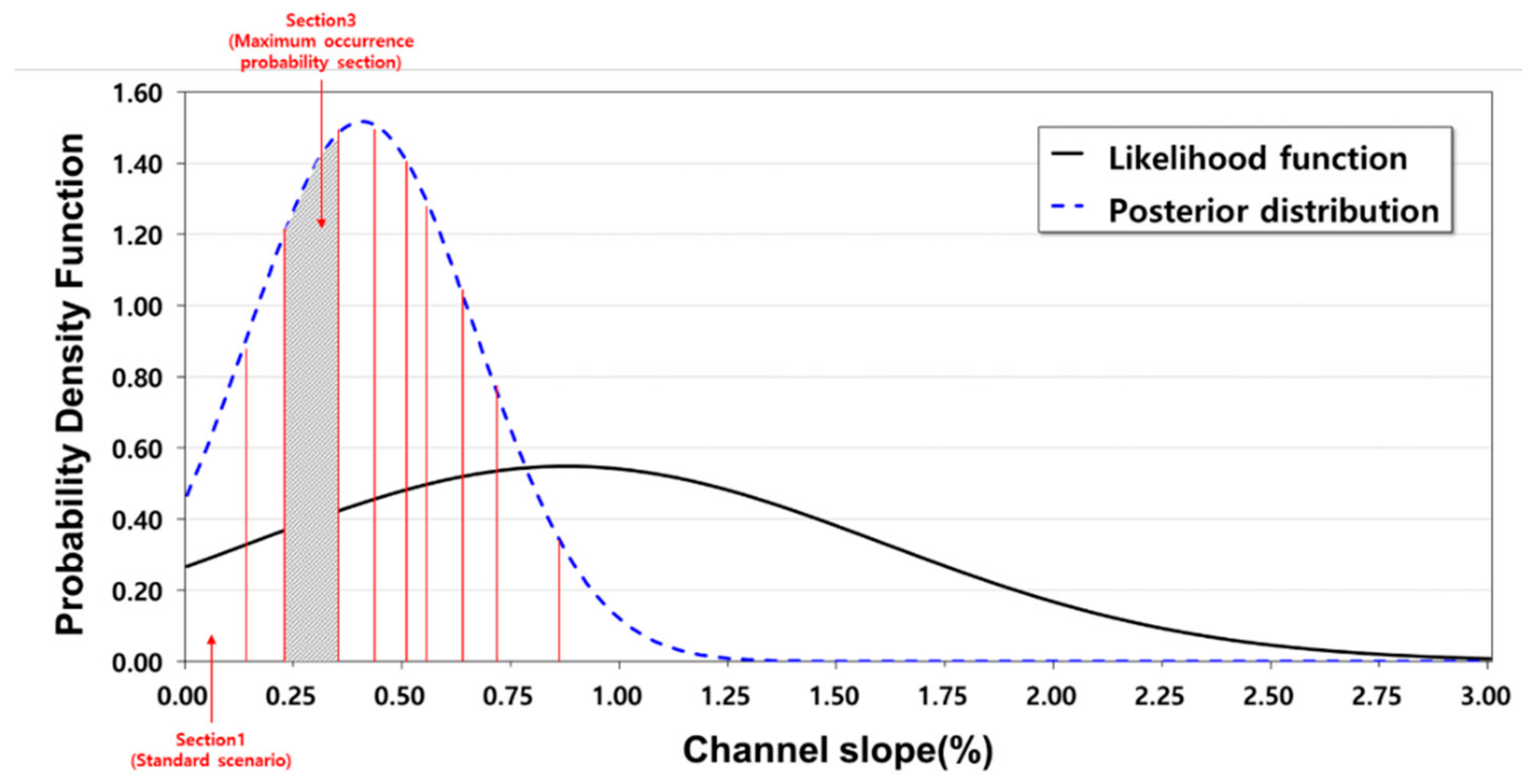
In this study, weights were determined through Bayesian inference to evaluation factors to determine the optimal design frequency in local river basins. First, the distribution parameters of the evaluation factors were estimated using the maximum likelihood method assuming they follow a normal distribution, as shown in Table 1. The posterior probability distribution of each indicator was estimated by applying its prior distribution and likelihood function to Equation (1). Figure 2 shows the likelihood function and posterior probability of the watershed area as an example.

Table 1.
Parameters of normal distribution for indicators.
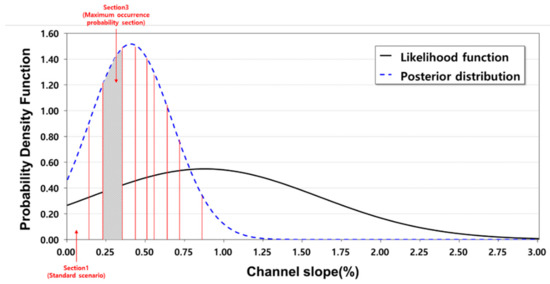
Figure 2.
Likelihood function and posterior distribution of channel slope.
To calculate the weights, considering the characteristics of data, watershed area, shape factor, river channel slopes, urban flooding areas, and extreme rainfall frequencies were divided into 10 equal parts, whereas the stream order and backwater effect reach were divided into five and two sections, respectively. The probability of occurrence for each part was determined by calculating the area of posterior probability distribution for each section. For example, river channel slope data were divided into 10 equal parts, the probability of occurrence of the safest is 0.07, and the maximum probability of occurrence is 0.18, which corresponds to the third. Therefore, the probability of occurrence of the channel slope was 0.82.
The final weights in Table 2 were obtained by calculating the ratios of each evaluation factor in total after calculating all the other evaluation factors. The score of watershed area was 15 points, and the score of the shape factor was 11 points, thus the score of watershed characteristics was 26 points. The total score of river characteristics was 38 points, with channel slope of 15, stream order of 12, and backwater effect reach of 11. The scores of the extreme rainfall frequency and the urban flooding area were both 18 points, thus the score of extreme flood characteristics was 36 points.

Table 2.
Ratio of occurrence probability and scores for indicators.
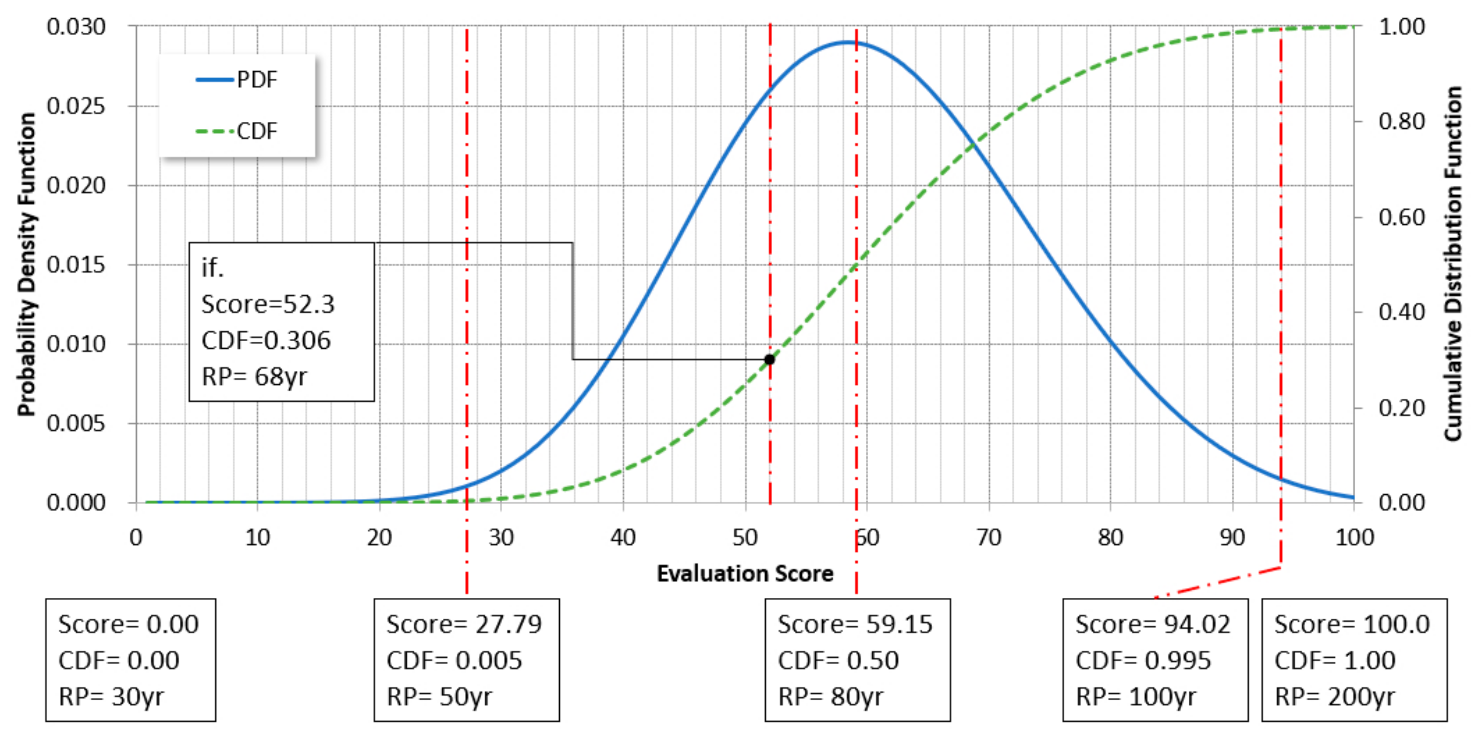
After calculating the scores using a score sheet for 413 local river basins in Chungcheongnam-do, the calculated scores were applied to the generalized extreme value (GEV) distribution. It was assumed that 99% of the cumulative distribution function (CDF) belongs to a return period range of 50–100 years, which is the general design frequency of local river basins. This assumption seems valid because there is no river corresponding to a return period of 200 years in Chungcheongnam-do. The scores corresponding to 0.005 and 0.995 of CFD are illustrated in Figure 3 and converted to the return periods of 50 and 100 years, respectively. For the score corresponding to 0.5 of CDF, the optimal design frequencies were estimated by assuming a return period of 80 years.
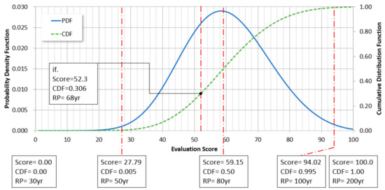
Figure 3.
GEV probability distribution for evaluation score.
The estimated return periods of 413 basins were compared with the existing ones which was estimated for previous studies in Chungcheongnam-do. The results of our study indicated that one river basin was estimated as return periods of 30–50 years, 195 river basins as return periods of 50–80 years, 213 river basins as return periods of 80–100 years, and four river basins as return periods of 100 years or more. All four river basins estimated as return periods of 100 years or more were rounded off from the return period of 99.95 years. No river basin was estimated to exceed the return period of 100 years. The return periods of this study were higher by approximately (+)7.62 years on average than the existing design frequencies.
As a result of estimating the design frequencies of local river basins, 255 river basins increased design frequencies and 158 river basins decreased design frequencies compared to the existing design frequencies. It is because that Chungcheongnam-do [3] determined the design frequencies corresponding to 30, 50, 80, 100, and 200 years of return periods using the CDFs of the normal distribution as a range after calculating the weights using the AHP. The weights of the evaluation factors in the AHP analysis are different from those of this study, and four design frequencies were selected using the PDF in addition to the scores. In other words, when the CDF was estimated by the scores of the return period of 50–80 years, the river basins were estimated to have a design frequency of 50 years or 80 years depending on the PDF. Hence, although the actual score of the evaluation factor was higher than the existing design frequency, the number of “the same” or “lower” river basins increased.
Among the river basins that showed a higher design return period in this study, the return period for Sapgyocheon was 99.46 years, but the existing return period was 50 years. This is because the urbanized area that corresponds to the main stream was very widely distributed, and the urban flooding area was 5,066,929 m2, which is more than double the “201,494 m2 or larger” standard corresponding to the perfect score (18 points, see Table 2). Among the river basins that showed a lower design frequency, the Namchangcheon is a very small river with a watershed area of 1.86 km2, but the design frequency was 80 years of a return period. The urban flooding area of the Namchangcheon was 2043 m2, and the stream order was 3. It was estimated to have a return period of 50.84 years because it was highly underestimated compared to the existing one.
The results showed that this study estimated higher frequencies than the existing design frequencies and the previous study [3]. The main difference between this study and the previous studies is that this study conducted quantitative evaluation by calculating weights through statistical inference for the evaluation factors, and the frequencies were derived using a score sheet rather than the range for the optimal design frequency.
4. Hydrological Risks According to Climate Change Scenarios
4.1. Generation of Daily Rainfall Time Series
In South Korea, the Korea Meteorological Administration (KMA) is responsible for producing climate change scenarios. KMA produces the RCP scenarios based on the 5th assessment report of the Intergovernmental Panel on Climate Change.
KMA provides the Coupled Model Intercomparison Project—Phase 5 (CMIP5)-based RCP scenarios. Using two general circulation models (GCM) (HadGEM2-AO and HadGEM2-ES, resolution = 1.875° × 1.250°), the APEC Climate Center provides a Korean climate change standard scenarios consisting of daily hydro-climatological data with same resolution with the automated surface observing system (ASOS) in South Korea. In this study, using the MBLRP model, daily rainfall time series provided by the Korean climate change standard scenarios were temporally downscaled to hourly unit corresponding to the ASOS in Chungcheongnam-do.
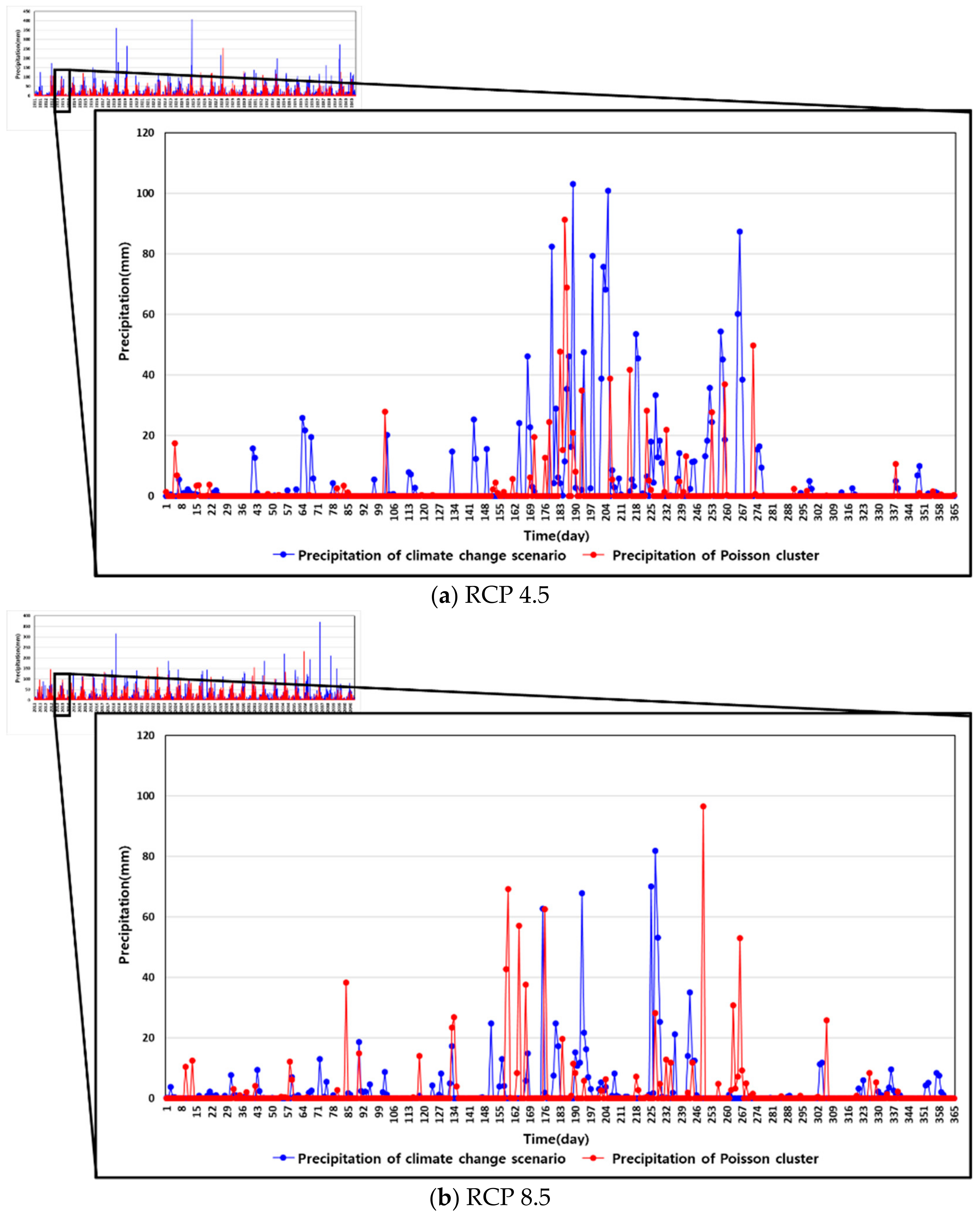
Table 3 and Figure 4 show representative results of the downscaling performance for the Cheongju station. It was found that the overall performance was excellent because the prediction performance of the hourly rainfall to which the Poisson cluster was applied was close to zero, and all the values were smaller than 10 mm/day [22]. Although performance results for two GCMSs were similar, the hourly rainfalls of HadGEM2-ES were used for further analyses in this study, which had better results on downscaling performance.

Table 3.
Performance results corresponding to GCM and RCP.
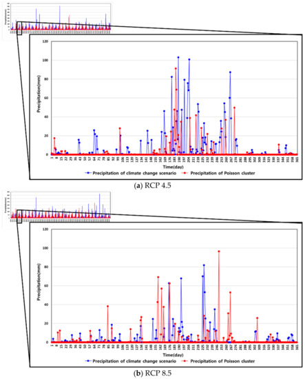
Figure 4.
Time series of rainfalls from the HadGEM2-ES for Cheongju station.
4.2. Estimation of Optimal Design Frequency According to Climate Change Scenarios
In this study, we applied climate change scenarios to the extreme rainfall frequency among the evaluation factors for estimating the optimal design frequency of local river basins. Hourly rainfall data were generated using the Poisson cluster model from the daily rainfall data of the future climate change scenario provided by the KMA. By analyzing future hourly rainfalls, the number of days of heavy rain alerts, the number of days of heavy rain warnings, the number of days of heavy rain over 50 mm, the number of days of heavy rain over 80 mm, and the number of days of heavy rain over 100 mm were calculated. Then, the extreme rainfall frequencies were calculated for each GCM model and future period. Furthermore, the urban flooding area for each local river basin was calculated by applying the rate of urbanization of future of Chungcheongnam-do.
The Environmental Geographic Information Service (EGIS) [23] (https://egis.me.go.kr, accessed on 27 March 2021) provides small-scale maps with a spatial resolution of 30 m, which are classified into seven factors (urbanized/dry area, agricultural area, forest area, grassland, wetland, bare area, and water area). The maps for the 1980s (photographed in 1987–1989), the 1990s (photographed in 1997–1999), and 2000s (photographed in 2008–2010) have been created, and the update period is 10 years. National land changes were analyzed using the land cover maps created in 10-year period to calculate the change at future time of the urbanized/dry areas among the time series changes of land cover. The urban area change rate was estimated by regression models and the rates of urban flooding area were estimated by using GIS software.
As a result of applying the climate change scenarios to evaluation factors for estimating the optimal design frequency of local river basins, Table 4 shows the number of river basins with changes (increase or decrease) in the estimated design frequency compared with the existing frequency according to the RCP 4.5 and 8.5. In the RCP 4.5 scenario, 269 basins had increased design frequencies in the P2, 195 basins had decreased design frequencies in the P1. In the RCP 8.5 scenario, 262 basins had increased design frequencies in the P1, 187 basins had decreased design frequencies in the P3. In addition, the estimated design frequencies were higher by (+)7.64 years on average (TP) for the RCP 4.5 and by (+)5.8 years for the RCP 8.5.

Table 4.
The number of river basins with changes in the estimated design frequency considering climate change scenarios (HadGEM2-ES).
In the RCP 4.5 scenario of the HadGEM2-ES GCM model, the values were concentrated at the center in P2, and widely distributed in the other periods. In the P1 period of the RCP 8.5 scenario, the values were relatively concentrated at the center in P1.
The above results indicated that the river basins vulnerable to flood will be more in the future than the current. Furthermore, it was predicted that the river basins will become more vulnerable to flood in the future periods.
4.3. Evaluation of Hydrological Risks According to Climate Change Scenarios
The hydrological risk means the probability of the occurrence of a hydrological event of a return period of T years at least once in n consecutive years. Therefore, hydrological risks should be considered in water control designs. Structures may be failed if a hydrological event with a design return period of T years occurs within the expected life span of the structure. Hydrological risks can be expressed as:
where is the risk, is the expected life time, and is the return period.
Hydrological risk increases as the return period and the expected life time increase. Therefore, the hydrological risk was calculated by applying the current design frequency to the return period T and by applying the estimated design frequency according to the climate change scenario to the expected time n.
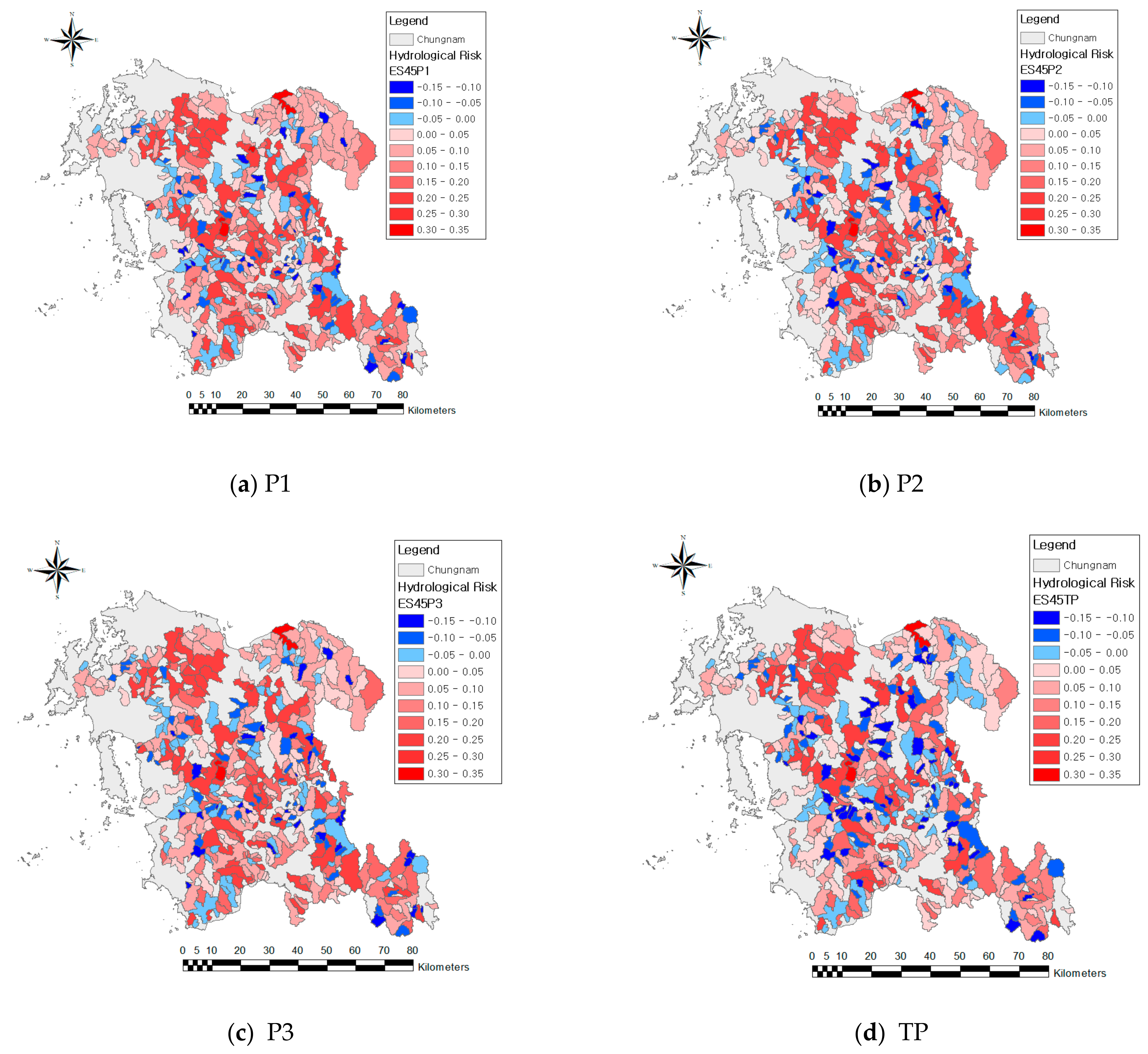
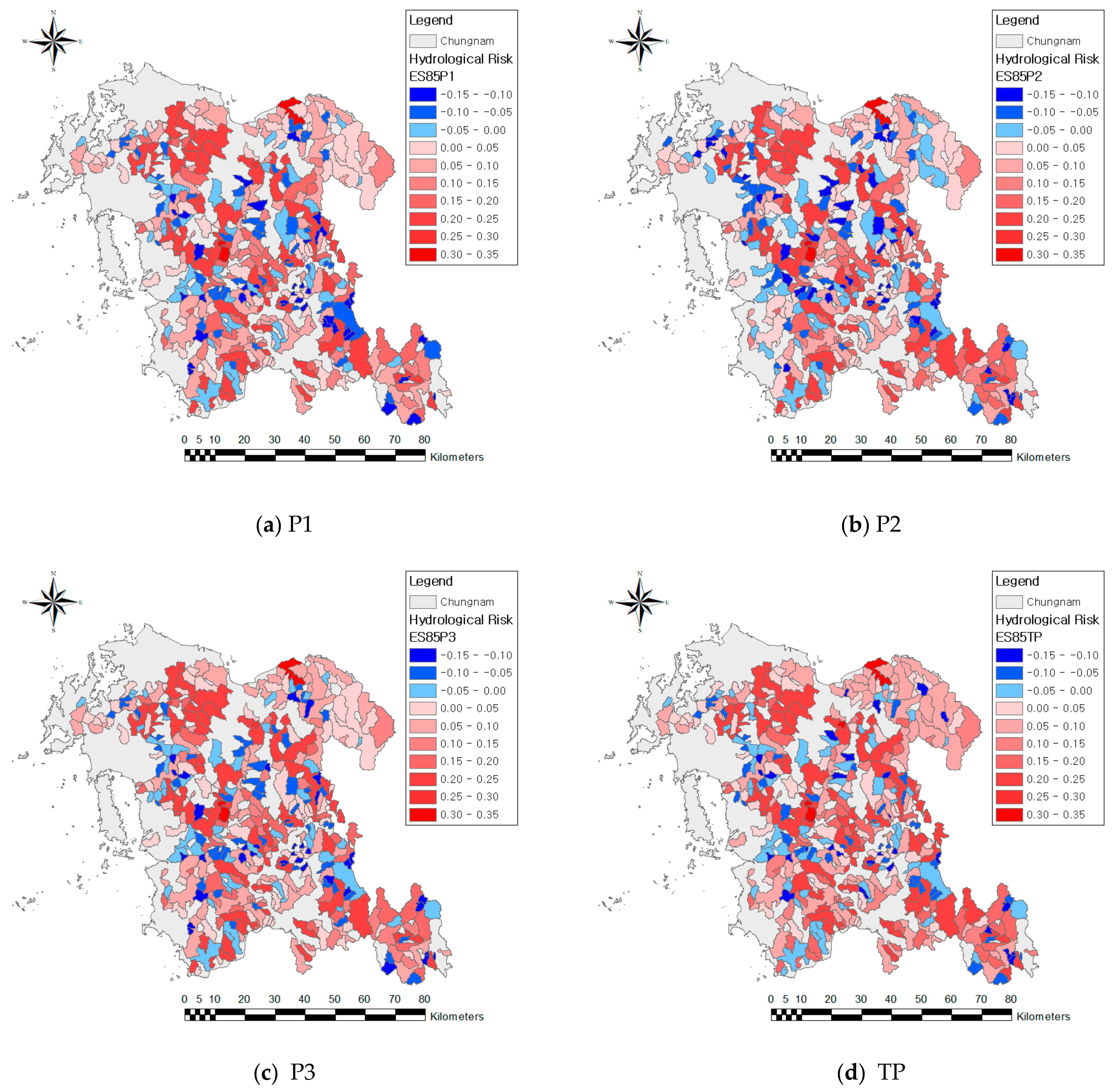
The hydrological risks were estimated for 413 local river basins in Chungcheongnam-do according to the GCM model, climate change scenario, and future period, and the results are shown in Figure 5 and Figure 6. As a result of evaluating the hydrological risks by applying future climate changes (Table 5), compared to the existing, the risk increased by 3.13% in the case of RCP 4.5, and by 2.80% in the case of RCP 8.5, on average. Especially, the risk increased by 4.58% in the P2 of RCP 4.5 and by 4.39% in the P1 of RCP 8.5.
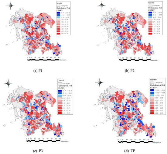
Figure 5.
Hydrologic risks for the RCP 4.5 (HadGEM2-ES).
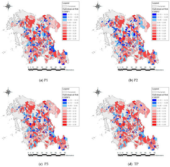
Figure 6.
Hydrologic risks for the RCP 8.5 (HadGEM2-ES).

Table 5.
Result of the average risk increase rate (%).
5. Conclusions
Flood damage is increasing worldwide due to irregular heavy storms caused by climate change. Although the South Korean government establishes flood control plans for local river basins considering the impact of climate change, the design frequency, which is the most basic design standard, is established based on river master plans established in the past. Until now, it was difficult to develop a practical, standardized method for calculating hydrologic design frequency for local river basins, although many efforts have been made to develop such a method in South Korea. Most of all, it was due to a lack of quantified and objective guidelines. This study determined the weighting values of evaluation factors such as watershed characteristics, river channel characteristics, extreme flood characteristics using Bayesian inference. From this, we estimated the optimal design frequencies of local river basins, and evaluated future flood risks. The conclusions derived from the results of this study are as follows:
- (1)
- Data for each evaluation factor were collected for 413 local river basins in Chungcheongnam-do, for which the basic plans were established. The evaluation sections were divided into equal parts, and weights were calculated using Bayesian theory. When the calculated optimal design frequencies were compared to the existing design frequencies, 253 river basins showed increased design frequencies and 160 river basins showed decreased design frequencies. The design frequency increased compared to that found by Chungcheongnam-do [3] because the urban areas of Chungcheongnam-do are relatively small. As a result, the weights for urban flooding area were calculated to be small.
- (2)
- This study secured statistical objectivity using Bayesian inference to complement the problem of weight calculation using the AHP used by Chungcheongnam-do [3]. However, in the case of urban flooding areas that were emphasized by many researchers, the weight was 18 points (in this study), which was highly underestimated compared to the 40-point weighting values in previous studies. This weight problem may be limited to Chungcheongnam-do, because the urban flooding area of Chungcheongnam-do is smaller than those of other municipalities. Therefore, if the urban flooding area increases beyond Chungcheongnam-do to metropolitan cities (which can be explored in future studies), it is expected that different weights will be derived.
- (3)
- The calculated hydrological flood risk showed that polarization will worsen with future climate change, and the risk increased by approximately 2.96% on average. This result indicates that the design frequency is likely to decrease in the future than in the present, and that the stability of flooding will decrease while the risk increases.
The findings of this study showed that even though hydrological risks calculated according to RCP scenarios may be partially different from those of previous studies, a relatively small risks were expected because the influence of factors excluding the increase in rainfall was considered when determining the hydrologic design frequency. These results can be utilized when estimating the hydrologic design frequency by securing statistical objectivity while excluding the field experience of designers in the process of establishing river master plans.
Author Contributions
Conceptualization, T.-W.K. and J.-Y.L.; methodology, J.-H.R. and J.-Y.L.; validation, J.-E.K. and H.-H.K.; formal analysis, J.-H.R.; investigation, J.-Y.L.; resources, J.-E.K.; data curation, J.-H.R.; writing—original draft preparation, J.-H.R.; writing—review and editing, T.-W.K. and H.-H.K.; visualization, J.-E.K.; supervision, T.-W.K.; project administration, J.-E.K. All authors have read and agreed to the published version of the manuscript.
Funding
This work was supported by the National Research Foundation of Korea (NRF) grant funded by the Korea government (MOE) (NRF-2020R1A2C1012919).
Institutional Review Board Statement
Not applicable.
Informed Consent Statement
Informed consent was obtained from all the subjects involved in the study.
Data Availability Statement
All the data used in the study are available online at http://www.data.kma.go.kr (accessed on 22 February 2021) and http://www.wamis.go.kr/Main.aspx (accessed on 27 March 2021).
Conflicts of Interest
The authors declare no conflict of interest.
References
- Hong, S.S.; Jung, D.S.; Hwang, E.H.; Chae, H.S. A study on the watershed analysis of the expected flood inundation area in South Han River. J. Korean Assoc. Geogr. Inf. Stud. 2016, 19, 106–119. [Google Scholar] [CrossRef]
- Ministry of the Interior and Safety. Disaster Annual Report; MOIS: Seoul, Korea, 2019.
- Ryu, J.H.; Lee, J.-Y.; Kim, J.E.; Kim, T.-W. Determination of the Optimal Return Period for River Design in Chungcheongnam-Do; CCND: Daejeon, Korea, 2017. [Google Scholar]
- Lee, E.H.; Choi, H.S.; Kim, J.H. Determination of flood risk considering flood control ability and urban environment risk. J. Korea Water Resour. Assoc. 2015, 48, 757–768. [Google Scholar] [CrossRef]
- Chen, Z.M.; Yeh, Y.L.; Chen, T.C. Assessment of a regional flood disaster indicator via an entropy weighting method. Nat. Hazards Rev. 2018, 19, 05018002. [Google Scholar] [CrossRef]
- Lee, J.; Jun, H.; Choi, J.; Park, J. Evaluation of urban small watershed relative flood risk using multi criteria decision making method. J. Korean Soc. Hazard Mitig. 2018, 18, 431–438. [Google Scholar] [CrossRef][Green Version]
- Joo, H.; Lee, T.; You, Y.; Wang, W.; Kim, S.; Kim, H.S. Determination of investment priority for flood control using flood risk and economic assessments. J. Korean Soc. Hazard Mitig. 2019, 19, 291–301. [Google Scholar] [CrossRef]
- Ministry of Public Safety and Security. Guideline for the Design Criteria of Structural Measures to Prevent Natural Disasters under Climate Change; MOPSS: Seoul, Korea, 2014.
- Kim, B.S.; Ha, S.R. The impact assessment of climate change on design flood in Mihochen basin based on the representative concentration pathway climate change scenario. J. Wetl. Res. 2013, 15, 105–114. [Google Scholar] [CrossRef][Green Version]
- Cha, W.Y.; Lee, O.J.; Kim, S.D.; Park, Y.K. Analysis of indicators of hydrological alteration on the Geumho river basin under AR5 RCP scenarios. J. Korean Soc. Hazard Mitig. 2017, 17, 317–326. [Google Scholar] [CrossRef]
- Kwon, M.; Lee, G.; Jun, K.S. Analysis of annual maximum daily rainfall using RCP climate change scenario in Korean peninsula. J. Korean Soc. Hazard Mitig. 2015, 15, 99–110. [Google Scholar] [CrossRef][Green Version]
- Lee, H.; Lee, T.; Park, T.; Son, C. Revisiting design flood estimation of Nam River Dam basin considering climate change. J. Korea Water Resour. Assoc. 2016, 49, 719–729. [Google Scholar] [CrossRef][Green Version]
- Lee, O.; Park, M.; Lee, J.; Kim, S. Future PMPs projection according to precipitation variation under RCP 8.5 climate change scenario. J. Korea Water Resour. Assoc. 2016, 49, 107–119. [Google Scholar] [CrossRef]
- Sim, K.B.; Lee, O.J.; Kim, S.D.; Kim, E.S. Analysis of future probable maximum precipitation using KMA AR5 1-km resolution RCP data. J. Korean Soc. Hazard Mitig. 2017, 17, 335–342. [Google Scholar] [CrossRef]
- Condon, L.E.; Gangopadhyay, S.; Pruitt, T. Climate change and non-stationary flood risk for the upper Truckee River basin. Hydrol. Earth Syst. Sci. 2015, 19, 159–175. [Google Scholar] [CrossRef]
- Kim, N.W.; Lee, J.Y.; Park, D.H.; Kim, T.W. Evaluation of future flood risk according to RCP scenarios using a regional flood frequency analysis for ungauged watersheds. Water 2019, 11, 992. [Google Scholar] [CrossRef]
- Lee, J.Y.; Son, H.J.; Kim, D.; Ryu, J.H.; Kim, T.W. Evaluating the hydrologic risk of n-year floods according to RCP scenarios. Water 2021, 13, 1805. [Google Scholar] [CrossRef]
- Rodriguez-Iturbe, I.; Cox, D.R.; Isham, V. Some models for rainfall based on stochastic point processes. Proceedings of the Royal Society of London. A. Math. Phys. Sci. 1987, 410, 269–288. [Google Scholar]
- Kim, J.G.; Kwon, H.H.; Kim, D. A development of hourly rainfall simulation technique based on Bayesian MBLRP model. KSCE J. Civ. Environ. Eng. Res. 2014, 34, 821–831. [Google Scholar]
- Ministry of Land, Infrastructure and Transport. List of Rivers in Korea; MOLIT: Seoul, Korea, 2018.
- Ministry of Land, Infrastructure and Transport. Insurance Rate Making and Mapping Based on Natural Disaster Risk; MOLIT: Seoul, Korea, 2018.
- Kim, Y.T.; Park, M.; Kwon, H.H. Optimization of PRISM parameters using the SCEM-UA algorithm for gridded daily time series precipitation. J. Korea Water Resour. Assoc. 2020, 53, 903–915. [Google Scholar]
- Environmental Geographic Information Service, EGIS. Available online: https://egis.me.go.kr (accessed on 21 December 2021).
Publisher’s Note: MDPI stays neutral with regard to jurisdictional claims in published maps and institutional affiliations. |
© 2022 by the authors. Licensee MDPI, Basel, Switzerland. This article is an open access article distributed under the terms and conditions of the Creative Commons Attribution (CC BY) license (https://creativecommons.org/licenses/by/4.0/).


