
Effects of Climate Change on Hydrology in the Most Relevant Mining Basin in the Eastern Legal Amazon

 , , ,
, , ,  , , and
Abstract
:
1. Introduction
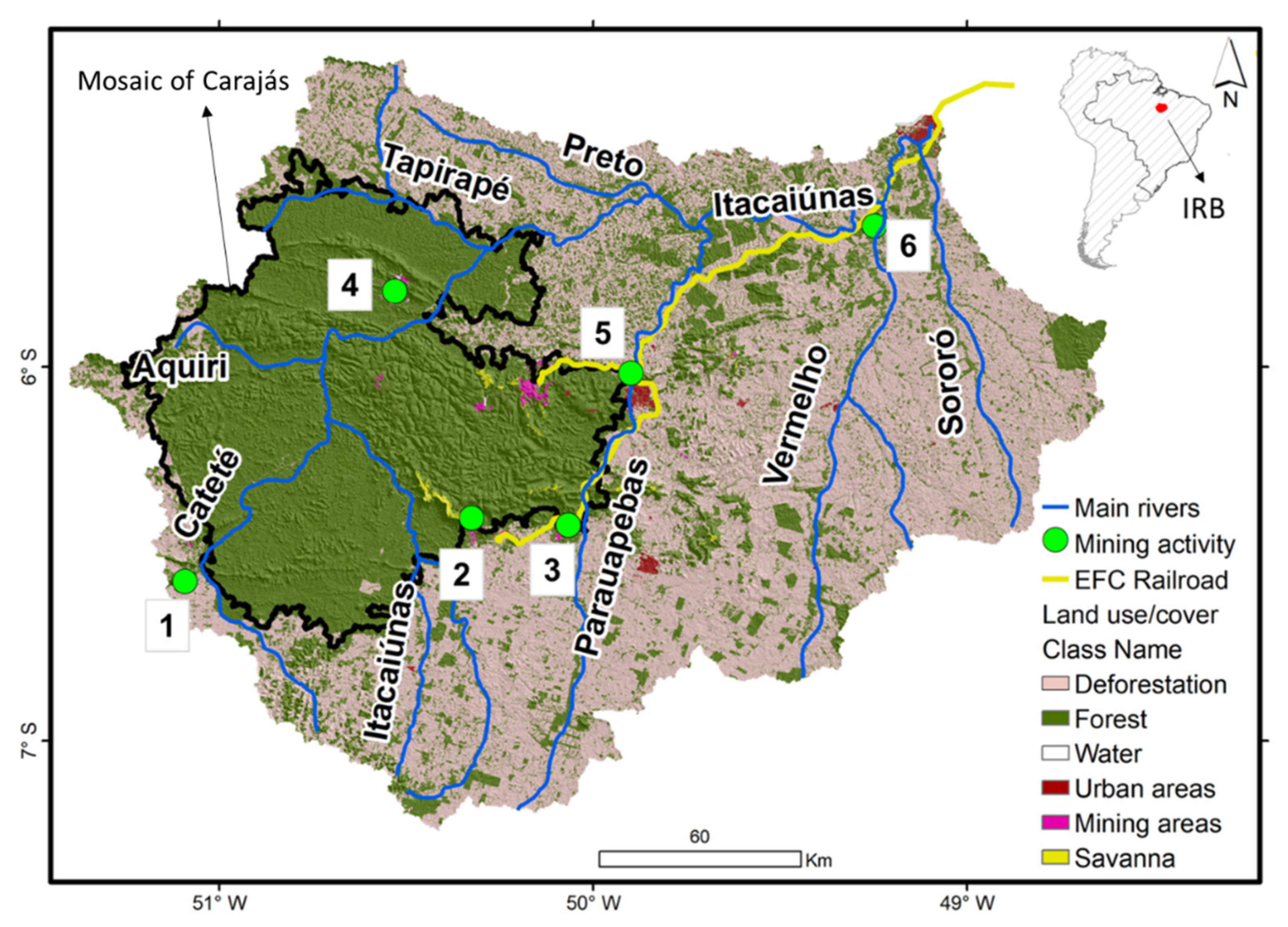
2. Study Area
3. Materials and Methods
3.1. Data Acquisition of GCMs
3.2. Simulation of Climate Change with the Hydrological Model
3.2.1. The MGB Large-Scale Hydrological Model
3.2.2. The MGB Model Setup
3.2.3. Assessment of Climate Change Impacts on Hydrological Processes
4. Results
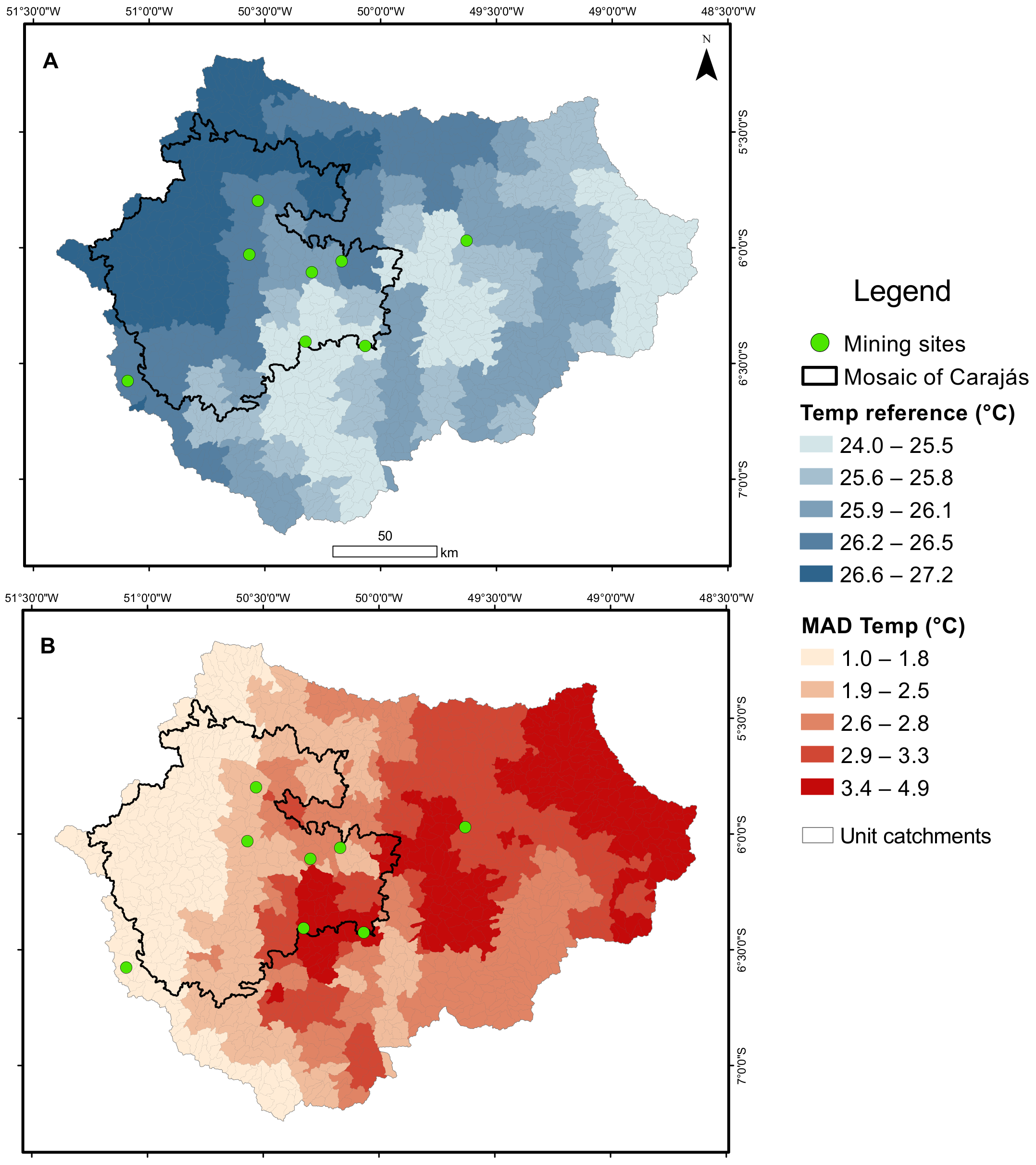
4.1. Air Temperature and Precipitation
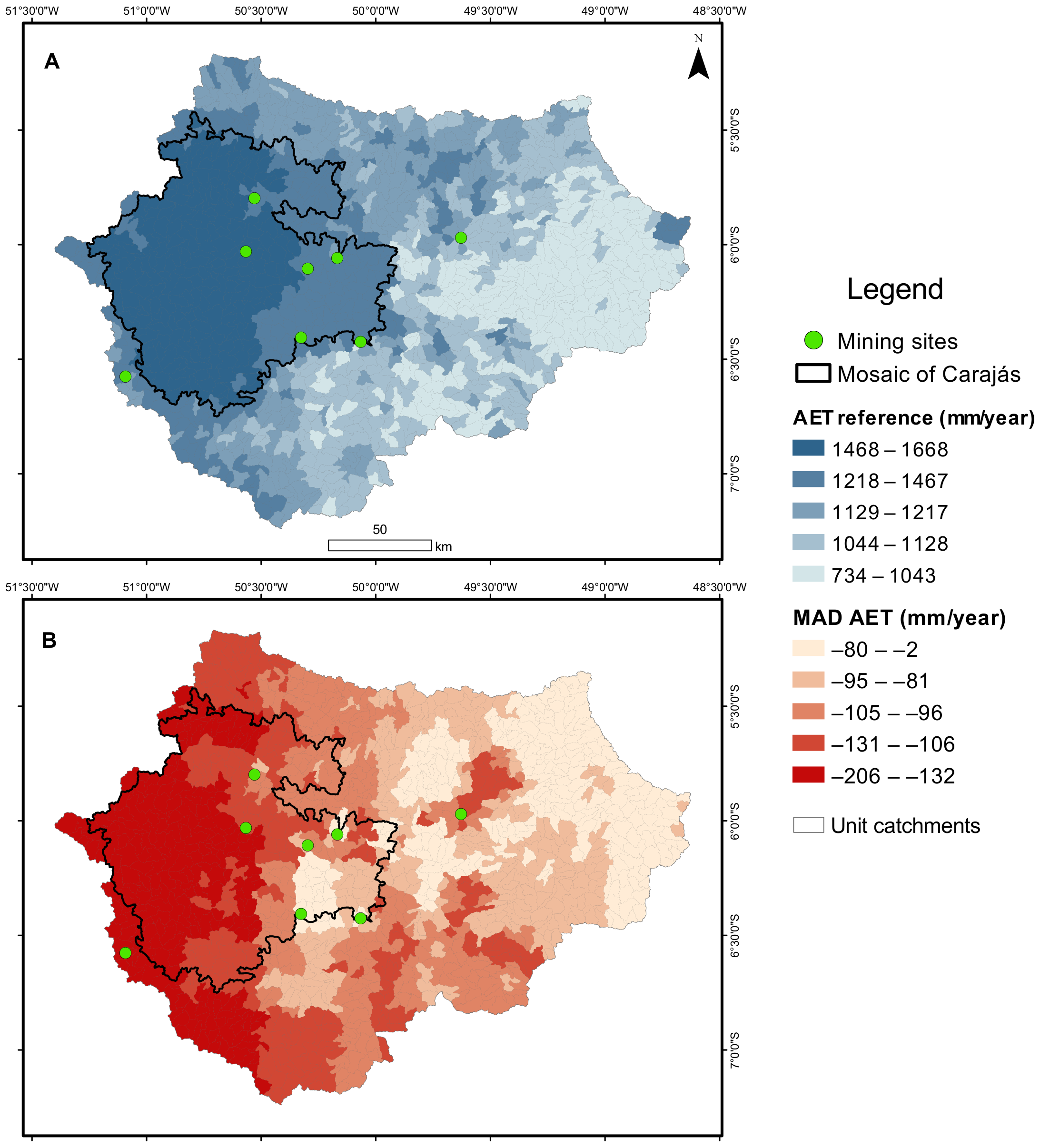
4.2. Evapotranspiration
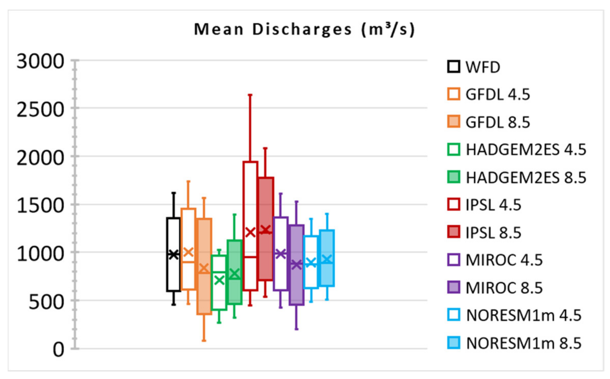
4.3. Discharges
5. Discussion
5.1. Hydrological Modeling and General Circulation Model Aspects
5.2. Practical Implications
6. Conclusions
Author Contributions
Funding
Acknowledgments
Conflicts of Interest
References
- Pearce, T.D.; Ford, J.D.; Prno, J.; Duerden, F.; Pittman, J.; Beaumier, M.; Berrang-Ford, L.; Smit, B. Climate change and mining in Canada. Mitig. Adapt. Strateg. Glob. Chang. 2011, 16, 347–368. [Google Scholar] [CrossRef]
- Panagoulia, D.; Bárdossy, A.; Lourmas, G. Diagnostic statistics of daily rainfall variability in an evolving climate. Adv. Geosci. 2006, 7, 349–354. [Google Scholar] [CrossRef] [Green Version]
- Mota, J.A.; Maneschy, M.C.; Souza-Filho, P.W.M.; Torres, V.F.N.; Siqueira, J.O.; Santos, J.F.D.; Matlaba, V. Uma nova proposta de indicadores de sustentabilidade na mineração. Sustentabilidade Debate 2017, 8, 15–29. [Google Scholar] [CrossRef] [Green Version]
- Batterham, R. Lessons in Sustainability from the Mining Industry. Procedia Eng. 2014, 83, 8–15. [Google Scholar] [CrossRef] [Green Version]
- Čuček, L.; Klemeš, J.; Kravanja, Z. A Review of Footprint analysis tools for monitoring impacts on sustainability. J. Clean. Prod. 2012, 34, 9–20. [Google Scholar] [CrossRef]
- Dialga, I. A Sustainability Index of Mining Countries. J. Clean. Prod. 2018, 179, 278–291. [Google Scholar] [CrossRef] [Green Version]
- Kunz, N.; Moran, C. Sharing the benefits from water as a new approach to regional water targets for mining companies. J. Clean. Prod. 2014, 84, 469–474. [Google Scholar] [CrossRef] [Green Version]
- Northey, S.; Mudd, G.; Saarivuori, E.; Wessman-Jääskeläinen, H.; Haque, N. Water footprinting and mining: Where are the limitations and opportunities? J. Clean. Prod. 2016, 135, 1098–1116. [Google Scholar] [CrossRef]
- Brechin, S.R.; Bhandari, M. Perceptions of climate change worldwide. Wiley Interdiscip. Rev. Clim. Chang. 2011, 2, 871–885. [Google Scholar] [CrossRef]
- Lobanova, A.; Liersch, S.; Nunes, J.P.; Didovets, I.; Stagl, J.; Huang, S.; Koch, H.; Rivas López, M.D.R.; Maule, C.F.; Hattermann, F.; et al. Hydrological impacts of moderate and high-end climate change across European river basins. J. Hydrol. Reg. Stud. 2018, 18, 15–30. [Google Scholar] [CrossRef]
- Mavume, A.F.; Banze, E.; Macie, O.A.; Queface, J. Analysis of Climate Change Projections for Mozambique under the Representative Concentration Pathways. Atmosphere 2021, 12, 588. [Google Scholar] [CrossRef]
- Rana, A.; Foster, K.; Bosshard, T.; Olsson, J.; Bengtsson, L. Impact of climate change on rainfall over Mumbai using Distribution-based Scaling of Global Climate Model projections. J. Hydrol. Reg. Stud. 2014, 1, 107–128. [Google Scholar] [CrossRef] [Green Version]
- Zheng, H.; Chiew, F.H.S.; Charles, S.; Podger, G. Future climate and runoff projections across South Asia from CMIP5 global climate models and hydrological modelling. J. Hydrol. Reg. Stud. 2018, 18, 92–109. [Google Scholar] [CrossRef]
- Siddique, R.; Karmalkar, A.; Sun, F.; Palmer, R. Hydrological extremes across the Commonwealth of Massachusetts in a changing climate. J. Hydrol. Reg. Stud. 2020, 32, 100733. [Google Scholar] [CrossRef]
- Chen, Y.; Velicogna, I.; Famiglietti, J.S.; Randerson, J.T. Satellite observations of terrestrial water storage provide early warning information about drought and fire season severity in the Amazon. J. Geophys. Res. Biogeosci. 2013, 118, 495–504. [Google Scholar] [CrossRef] [Green Version]
- Rowland, L.; Da Costa, A.C.L.; Galbraith, D.R.; Oliveira, R.S.; Binks, O.J.; Oliveira, A.A.R.; Pullen, A.M.; Doughty, C.E.; Metcalfe, D.B.; Vasconcelos, S.S.; et al. Death from drought in tropical forests is triggered by hydraulics not carbon starvation. Nature 2015, 528, 119–122. [Google Scholar] [CrossRef] [Green Version]
- Ndiaye, P.M.; Bodian, A.; Diop, L.; Dezetter, A.; Guilpart, E.; Deme, A.; Ogilvie, A. Future trend and sensitivity analysis of evapotranspiration in the Senegal River Basin. J. Hydrol. Reg. Stud. 2021, 35, 100820. [Google Scholar] [CrossRef]
- Greve, P.; Kahil, T.; Mochizuki, J.; Schinko, T.; Satoh, Y.; Burek, P.; Fischer, G.; Tramberend, S.; Burtscher, R.; Langan, S.; et al. Global assessment of water challenges under uncertainty in water scarcity projections. Nat. Sustain. 2018, 1, 486–494. [Google Scholar] [CrossRef]
- Odell, S.D.; Bebbington, A.; Frey, K.E. Mining and climate change: A review and framework for analysis. Extr. Ind. Soc. 2018, 5, 201–214. [Google Scholar] [CrossRef]
- Schewe, J.; Heinke, J.; Gerten, D.; Haddeland, I.; Arnell, N.W.N.W.; Clark, D.B.D.B.; Dankers, R.; Eisner, S.; Fekete, B.M.; Colón-González, F.J.F.J.; et al. Multimodel assessment of water scarcity under climate change. Proc. Natl. Acad. Sci. USA 2013, 104, 20167–20172. [Google Scholar] [CrossRef] [Green Version]
- Woznicki, S.A.; Nejadhashemi, A.P.; Parsinejad, M. Climate change and irrigation demand: Uncertainty and adaptation. J. Hydrol. Reg. Stud. 2015, 3, 247–264. [Google Scholar] [CrossRef]
- Bond, R.M.; Stubblefield, A.P.; Van Kirk, R.W. Sensitivity of summer stream temperatures to climate variability and riparian reforestation strategies. J. Hydrol. Reg. Stud. 2015, 4, 267–279. [Google Scholar] [CrossRef] [Green Version]
- Giannini, T.C.; Giulietti, A.M.; Harley, R.M.; Viana, P.L.; Jaffe, R.; Alves, R.; Pinto, C.E.; Mota, N.F.O.; Caldeira, C.F.; Imperatriz-Fonseca, V.L.; et al. Selecting plant species for practical restoration of degraded lands using a multiple-trait approach. Austral Ecol. 2017, 42, 510–521. [Google Scholar] [CrossRef]
- Meixner, T.; Manning, A.H.; Stonestrom, D.A.; Allen, D.M.; Ajami, H.; Blasch, K.W.; Brookfield, A.E.; Castro, C.L.; Clark, J.F.; Gochis, D.J.; et al. Implications of projected climate change for groundwater recharge in the western United States. J. Hydrol. 2016, 534, 124–138. [Google Scholar] [CrossRef] [Green Version]
- Pletterbauer, F.; Melcher, A.; Graf, W. Climate Change Impacts in Riverine Ecosystems. In Riverine Ecosystem Management; Aquatic Ecology Series; Schmutz, S., Sendzimir, J., Eds.; Springer: Cham, Switzerland, 2018; Volume 8. [Google Scholar] [CrossRef]
- Brêda, J.P.L.F.; de Paiva, R.C.D.; Collischon, W.; Bravo, J.M.; Siqueira, V.A.; Steinke, E.B. Climate change impacts on South American water balance from a continental-scale hydrological model driven by CMIP5 projections. Clim. Chang. 2020, 159, 503–522. [Google Scholar] [CrossRef]
- Alves, L.M.; Chadwick, R.; Moise, A.; Brown, J.; Marengo, J.A. Assessment of rainfall variability and future change in Brazil across multiple timescales. Int. J. Climatol. 2021, 41, E1875–E1888. [Google Scholar] [CrossRef]
- Sorribas, M.V.; Paiva, R.C.D.; Melack, J.M.; Bravo, J.M.; Jones, C.; Carvalho, L.; Beighley, E.; Forsberg, B.; Costa, M.H. Projections of climate change effects on discharge and inundation in the Amazon basin. Clim. Chang. 2016, 136, 555–570. [Google Scholar] [CrossRef]
- Magrin, G.O.; Marengo, J.; Boulanger, J.P.; Buckeridge, M.S.; Castellano, E.; Poveda, G.; Scarano, F.R.; Vicuña, S.; Alfaro, E.; Anthelme, F.; et al. Central and South America. In Climate Change 2014: Impacts, Adaptation, and Vulnerability. Part B: Regional Aspects. Contribution of Working Group II to the Fifth Assessment Report of the Intergovernmental Panel on Climate Change; Field, C.B., Barros, V.R., Dokken, D.J., Mach, K.J., Mastrandrea, M.D., Bilir, T.E., Chatterjee, M., Ebi, K.L., Estrada, Y.O., Genova, R.C., et al., Eds.; Cambridge University Press: Cambridge, UK, 2014; pp. 1499–1566. [Google Scholar]
- Barichivich, J.; Gloor, E.; Peylin, P.; Brienen, R.J.W.; Schöngart, J.; Espinoza, J.C.; Pattnayak, K.C. Recent intensification of Amazon flooding extremes driven by strengthened Walker circulation. Sci. Adv. 2018, 4, eaat8785. [Google Scholar] [CrossRef] [Green Version]
- Butt, M.J.; Umar, M.; Qamar, R. Landslide dam and subsequent dam-break flood estimation using HEC-RAS model in Northern Pakistan. Nat. Hazards 2013, 65, 241–254. [Google Scholar] [CrossRef]
- Espinoza, J.C.; Ronchail, J.; Marengo, J.A.; Segura, H. Contrasting North–South changes in Amazon wet-day and dry-day frequency and related atmospheric features (1981–2017). Clim. Dyn. 2019, 52, 5413–5430. [Google Scholar] [CrossRef]
- Leite-Filho, A.T.; Costa, M.H.; Fu, R. The southern Amazon rainy season: The role of deforestation and its interactions with large-scale mechanisms. Int. J. Climatol. 2020, 40, 2328–2341. [Google Scholar] [CrossRef]
- Marengo, J.A.; Chou, S.C.; Kay, G.; Alves, L.M.; Pesquero, J.F.; Soares, W.R.; Santos, D.C.; Lyra, A.A.; Sueiro, G.; Betts, R.; et al. Development of regional future climate change scenarios in South America using the Eta CPTEC/HadCM3 climate change projections: Climatology and regional analyses for the Amazon, São Francisco and the Paraná River basins. Clim. Dyn. 2012, 38, 1829–1848. [Google Scholar] [CrossRef]
- Ronchail, J.; Espinoza, J.C.; Drapeau, G.; Sabot, M.; Cochonneau, G.; Schor, T. The flood recession period in Western Amazonia and its variability during the 1985–2015 period. J. Hydrol. Reg. Stud. 2018, 15, 16–30. [Google Scholar] [CrossRef]
- Tomasella, J.; Borma, L.S.; Marengo, J.A.; Rodriguez, D.A.; Cuartas, L.A.; Nobre, C.A.; Prado, M.C.R. The droughts of 1996–1997 and 2004–2005 in Amazonia: Hydrological response in the river main-stem. Hydrol. Processes 2011, 25, 1228–1242. [Google Scholar] [CrossRef]
- De Amorim, P.B.; Chaffe, P.L.B. Integrating climate models into hydrological modelling: What’s going on in Brazil? Rev. Bras. Recur. Hidr. 2019, 24, e31. [Google Scholar] [CrossRef] [Green Version]
- OECD. Regulatory Governance in the Mining Sector in Brazil; OECD Publishing: Paris, France, 2022. [Google Scholar] [CrossRef]
- Pontes, P.R.M.; Cavalcante, R.B.L.; Sahoo, P.K.; Silva Júnior, R.O.D.; da Silva, M.S.; Dall’Agnol, R.; Siqueira, J.O. The role of protected and deforested areas in the hydrological processes of Itacaiúnas River Basin, eastern Amazonia. J. Environ. Manag. 2019, 235, 488–499. [Google Scholar] [CrossRef]
- Souza-Filho, P.W.M.; Nascimento, W.R.; Santos, D.C.; Weber, E.J.; Silva, R.O.; Siqueira, J.O. A GEOBIA approach for multitemporal land-cover and land-use change analysis in a tropical watershed in the southeastern Amazon. Remote Sens. 2018, 10, 1683. [Google Scholar] [CrossRef] [Green Version]
- Alvares, C.A.; Stape, J.L.; Sentelhas, P.C.; De Moraes Gonçalves, J.L.; Sparovek, G. Köppen’s climate classification map for Brazil. Meteorol. Z. 2013, 22, 711–728. [Google Scholar] [CrossRef]
- Cavalcante, R.B.L.; Pontes, P.R.M.; Souza-Filho, P.W.M.; de Souza, E.B. Opposite Effects of Climate and Land Use Changes on the Annual Water Balance in the Amazon Arc of Deforestation. Water Resour. Res. 2019, 55, 3092–3106. [Google Scholar] [CrossRef]
- Taylor, K.E.; Stouffer, R.J.; Meehl, G.A. An overview of CMIP5 and the experiment design. Bull. Am. Meteorol. Soc. 2012, 93, 485–498. [Google Scholar] [CrossRef] [Green Version]
- Hempel, S.; Frieler, K.; Warszawski, L.; Schewe, J.; Piontek, F. A trend-preserving bias correction—The ISI-MIP approach. Earth Syst. Dynam. 2013, 4, 219–236. [Google Scholar] [CrossRef] [Green Version]
- Collischonn, W.; Allasia, D.; Da Silva, B.C.; Tucci, C.E.M. The MGB-IPH model for large-scale rainfall—Runoff modelling. Hydrol. Sci. J. 2007, 52, 878–895. [Google Scholar] [CrossRef] [Green Version]
- Pontes, P.R.M.; Fan, F.M.; Fleischmann, A.S.; de Paiva, R.C.D.; Buarque, D.C.; Siqueira, V.A.; Jardim, P.F.; Sorribas, M.V.; Collischonn, W. MGB-IPH model for hydrological and hydraulic simulation of large floodplain river systems coupled with open source GIS. Environ. Model. Softw. 2017, 94, 1–20. [Google Scholar] [CrossRef]
- Siqueira, V.; Paiva, R.; Fleischmann, A.; Fan, F.; Ruhoff, A.; Pontes, P.; Paris, A.; Calmant, S.; Collischonn, W. Toward continental hydrologic–hydrodynamic modeling in South America. Hydrol. Earth Syst. Sci. Discuss. 2018, 22, 4815–4842. [Google Scholar] [CrossRef] [Green Version]
- Fleischmann, A.; Siqueira, V.; Paris, A.; Collischonn, W.; Paiva, R.; Pontes, P.; Crétaux, J.-F.; Bergé-Nguyen, M.; Biancamaria, S.; Gosset, M.; et al. Modelling hydrologic and hydrodynamic processes in basins with large semi-arid wetlands. J. Hydrol. 2018, 561, 943–959. [Google Scholar] [CrossRef]
- Wigmosta, M.S.; Vail, L.W.; Lettenmaier, D.P. A distributed hydrology–vegetation model for complex terrain. Water Resour. Res. 1994, 30, 1665–1679. [Google Scholar] [CrossRef]
- Todini, E. The ARNO rainfall-runoff model. J. Hydrol. 1996, 175, 339–382. [Google Scholar] [CrossRef]
- Takaku, J.; Tadono, T.; Tsutsui, K.; Ichikawa, M. Validation of “Aw3D” Global Dsm Generated from Alos Prism. ISPRS Annals of Photogrammetry, Remote Sensing and Spatial Information Sciences. In Proceedings of the XXIII ISPRS Congress, Prague, Czech Republic, 12–19 July 2016; Volume III–4, pp. 25–31. [Google Scholar] [CrossRef]
- O’Loughlin, F.E.; Paiva, R.C.D.; Durand, M.; Alsdorf, D.E.; Bates, P.D. A multi-sensor approach towards a global vegetation corrected SRTM DEM product. Remote Sens. Environ. 2016, 182, 49–59. [Google Scholar] [CrossRef] [Green Version]
- Nobre, A.D.; Cuartas, L.A.; Hodnett, M.; Rennó, C.D.; Rodrigues, G.; Silveira, A.; Waterloo, M.; Saleska, S. Height Above the Nearest Drainage—A hydrologically relevant new terrain model. J. Hydrol. 2011, 404, 13–29. [Google Scholar] [CrossRef] [Green Version]
- Yamazaki, D.; De Almeida, G.A.M.; Bates, P.D. Improving computational efficiency in global river models by implementing the local inertial flow equation and a vector-based river network map. Water Resour. Res. 2013, 49, 7221–7235. [Google Scholar] [CrossRef]
- Cavalcante, R.B.L.; Pontes, P.R.M.; Tedeschi, R.G.; Costa, C.P.W.; Ferreira, D.B.S.; Souza-Filho, P.W.M.; de Souza, E.B. Terrestrial water storage and Pacific SST affect the monthly water balance of Itacaiúnas River Basin (Eastern Amazonia). Int. J. Climatol. 2020, 40, 3021–3035. [Google Scholar] [CrossRef]
- Collischonn, B.; Collischonn, W. Rainfall as proxy for evapotranspiration predictions. Proc. Int. Assoc. Hydrol. Sci. 2016, 374, 35–40. [Google Scholar] [CrossRef] [Green Version]
- Escobar, H. Deforestation in the Brazilian Amazon is still rising sharply. Science 2020, 369, 613. [Google Scholar] [CrossRef]
- Giannini Costa, W.F.; Borges, R.C.; Miranda, L.; da Costa, C.P.W.; Saraiva, A.M.; Imperatriz Fonseca, V.L. Climate change in the Eastern Amazon: Crop-pollinator and occurrence-restricted bees are potentially more affected. Reg. Environ. Chang. 2020, 20, 9. [Google Scholar] [CrossRef] [Green Version]
- Jaffé, R.; Veiga, J.C.; Pope, N.S.; Lanes, É.C.M.; Carvalho, C.S.; Alves, R.; Andrade, S.C.S.; Arias, M.C.; Bonatti, V.; Carvalho, A.T.; et al. Landscape genomics to the rescue of a tropical bee threatened by habitat loss and climate change. Evol. Appl. 2019, 12, 1164–1177. [Google Scholar] [CrossRef] [Green Version]
- Miranda, L.S.; Imperatriz-Fonseca, V.L.; Giannini, T.C. Climate change impact on ecosystem functions provided by birds in southeastern Amazonia. PLoS ONE 2019, 14, e215229. [Google Scholar] [CrossRef] [Green Version]
- Boisier, J.P.; Ciais, P.; Ducharne, A.; Guimberteau, M. Projected strengthening of Amazonian dry season by constrained climate model simulations. Nat. Clim. Chang. 2015, 5, 656–660. [Google Scholar] [CrossRef]
- Llopart, M.; Simões Reboita, M.; Porfírio da Rocha, R. Assessment of multi-model climate projections of water resources over South America CORDEX domain. Clim. Dyn. 2020, 54, 99–116. [Google Scholar] [CrossRef]
- Her, Y.; Yoo, S.H.; Cho, J.; Hwang, S.; Jeong, J.; Seong, C. Uncertainty in hydrological analysis of climate change: Multi-parameter vs. multi-GCM ensemble predictions. Sci. Rep. 2019, 9, 4974. [Google Scholar] [CrossRef] [Green Version]
- Yin, L.; Fu, R.; Shevliakova, E.; Dickinson, R.E. How well can CMIP5 simulate precipitation and its controlling processes over tropical South America? Clim. Dyn. 2013, 41, 3127–3143. [Google Scholar] [CrossRef] [Green Version]
- Ho, J.T.; Thompson, J.R.; Brierley, C. Projections of hydrology in the Tocantins-Araguaia Basin, Brazil: Uncertainty assessment using the CMIP5 ensemble. Hydrol. Sci. J. 2016, 61, 551–567. [Google Scholar] [CrossRef]
- Belk, E.L.; Markewitz, D.; Rasmussen, T.C.; Carvalho, E.J.M.; Nepstad, D.C.; Davidson, E.A. Modeling the effects of throughfall reduction on soil water content in a Brazilian Oxisol under a moist tropical forest. Water Resour. Res. 2007, 43, W08432. [Google Scholar] [CrossRef]
- Christoffersen, B.O.; Restrepo-Coupe, N.; Arain, M.A.; Baker, I.T.; Cestaro, B.P.; Ciais, P.; Fisher, J.B.; Galbraith, D.; Guan, X.; Gulden, L.; et al. Mechanisms of water supply and vegetation demand govern the seasonality and magnitude of evapotranspiration in Amazonia and Cerrado. Agric. For. Meteorol. 2014, 191, 33–50. [Google Scholar] [CrossRef]
- Negrón Juárez, R.I.; Hodnett, M.G.; Fu, R.; Gouden, M.L.; von Randow, C. Control of dry season evapotranspiration over the Amazonian forest as inferred from observation at a Southern Amazon forest site. J. Clim. 2007, 20, 2827–2839. [Google Scholar] [CrossRef] [Green Version]
- Gao, C.; Liu, L.; Ma, D.; He, K.; Xu, Y.P. Assessing responses of hydrological processes to climate change over the southeastern Tibetan Plateau based on resampling of future climate scenarios. Sci. Total Environ. 2019, 664, 737–752. [Google Scholar] [CrossRef]
- Gesualdo, G.C.; Oliveira, P.T.; Rodrigues, D.B.B.; Gupta, H.V. Assessing water security in the São Paulo metropolitan region under projected climate change. Hydrol. Earth Syst. Sci. 2019, 23, 4955–4968. [Google Scholar] [CrossRef] [Green Version]
- Hoang, L.P.; van Vliet, M.T.H.; Kummu, M.; Lauri, H.; Koponen, J.; Supit, I.; Leemans, R.; Kabat, P.; Ludwig, F. The Mekong’s future flows under multiple drivers: How climate change, hydropower developments and irrigation expansions drive hydrological changes. Sci. Total Environ. 2019, 649, 601–609. [Google Scholar] [CrossRef]
- Wada, Y.; Bierkens, M.F.P. Sustainability of global water use: Past reconstruction and future projections. Environ. Res. Lett. 2014, 9, 104003. [Google Scholar] [CrossRef]
- Xu, R.; Hu, H.; Tian, F.; Li, C.; Khan, M.Y.A. Projected climate change impacts on future streamflow of the Yarlung Tsangpo-Brahmaputra River. Glob. Planet. Chang. 2019, 175, 144–159. [Google Scholar] [CrossRef] [Green Version]


| ID | Description |
|---|---|
| 1 | Mining site: Downstream Onça-Puma |
| 2 | Mining site: Downstream S11D |
| 3 | Mining site: Downstream Sossego |
| 4 | Mining site: Downstream Salobo |
| 5 | Mining influence: Confluence Gelado × Parauapebas rivers |
| 6 | Mining railroad: Vermelho river |
| GCM | Spatial Resolution (Available in Earth System Grid Federation) | Institute | Country |
|---|---|---|---|
| GFDL-ESM2 M | 0.5° × 0.5° | NOAA GFDL | United States |
| HADGEM2ES | 0.5° × 0.5° | UK Met Office | United Kingdom |
| IPSL-CM5A-LR | 0.5° × 0.5° | IPSL | France |
| MIROC-ESM-CHEM | 0.5° × 0.5° | MIROC | Japan |
| NorESM1-M | 0.5° × 0.5° | NorESM | Norway |
| Time Period | Data Source | Annual Precipitation (mm/Year) | Mean Annual Temperature (°C) | ||
|---|---|---|---|---|---|
| RCP4.5 | RCP8.5 | RCP4.5 | RCP8.5 | ||
| 1971–2001 | WFD | 1937.8 | 25.9 | ||
| 2021–2050 | GFDL | 1756.9 | 1635.4 | 27.8 | 28.1 |
| HADGEM2ES | 1760.7 | 1745.4 | 28.5 | 28.8 | |
| IPSL | 1822.7 | 1928.0 | 28.2 | 28.5 | |
| MIROC | 1880.0 | 1758.7 | 28.2 | 29.2 | |
| NORESM1 m | 1861.5 | 1840.9 | 27.8 | 28.1 | |
| Mean of GCMs | 1816.4 | 1781.7 | 28.1 | 28.6 | |
| MRD between Mean GCMs and WFD | −6% | −8% | 8% | 10% | |
| Time Period | Data Source | Annual AET (mm/Year) | |
|---|---|---|---|
| RCP4.5 | RCP8.5 | ||
| 1971–2001 | WFD | 1218.4 | |
| 2021–2050 | GFDL | 1050.2 | 1025.4 |
| HADGEM2ES | 1204.9 | 1190.6 | |
| IPSL | 1050.9 | 1068.9 | |
| MIROC | 1140.2 | 1115.2 | |
| NORESM1 m | 1185.6 | 1161.9 | |
| Mean of GCMs | 1126.3 | 1112.4 | |
| MRD between Mean GCMs and WFD | −8% | −9% | |
| Time Period | Data Source | Discharge (m3/s) | |
|---|---|---|---|
| RCP4.5 | RCP8.5 | ||
| 1971–2001 | WFD | 946 | |
| 2021–2050 | GFDL | 973 | 828 |
| HADGEM2ES | 723 | 748 | |
| IPSL | 1028 | 1203 | |
| MIROC | 975 | 867 | |
| NORESM1 m | 896 | 912 | |
| Mean of GCMs | 919 | 911 | |
| MRD between Mean GCMs and WFD | −3% | −4% | |
| ID | Mean Relative Differences Q90 (%) | Mean Relative Differences Q5 (%) | ||
|---|---|---|---|---|
| RCP 4.5 | RCP 8.5 | RCP 4.5 | RCP 8.5 | |
| 1 | −67.0 | −75.4 | 0.8 | 1.3 |
| 2 | −90.1 | −96.7 | 0.2 | 2.3 |
| 3 | −61.0 | −69.4 | 3.2 | 3.4 |
| 4 | −86.4 | −93.6 | 2.6 | 5.3 |
| 5 | −75.5 | −85.1 | 4.7 | 8.1 |
| 6 | −55.6 | −63.8 | 3.8 | 6.6 |
Publisher’s Note: MDPI stays neutral with regard to jurisdictional claims in published maps and institutional affiliations. |
© 2022 by the authors. Licensee MDPI, Basel, Switzerland. This article is an open access article distributed under the terms and conditions of the Creative Commons Attribution (CC BY) license (https://creativecommons.org/licenses/by/4.0/).
Share and Cite
Pontes, P.R.M.; Cavalcante, R.B.L.; Giannini, T.C.; Costa, C.P.W.; Tedeschi, R.G.; Melo, A.M.Q.; Xavier, A.C.F. Effects of Climate Change on Hydrology in the Most Relevant Mining Basin in the Eastern Legal Amazon. Water 2022, 14, 1416. https://doi.org/10.3390/w14091416
Pontes PRM, Cavalcante RBL, Giannini TC, Costa CPW, Tedeschi RG, Melo AMQ, Xavier ACF. Effects of Climate Change on Hydrology in the Most Relevant Mining Basin in the Eastern Legal Amazon. Water. 2022; 14(9):1416. https://doi.org/10.3390/w14091416
Chicago/Turabian StylePontes, Paulo Rogenes M., Rosane B. L. Cavalcante, Tereza C. Giannini, Cláudia P. W. Costa, Renata G. Tedeschi, Adayana M. Q. Melo, and Ana Carolina Freitas Xavier. 2022. "Effects of Climate Change on Hydrology in the Most Relevant Mining Basin in the Eastern Legal Amazon" Water 14, no. 9: 1416. https://doi.org/10.3390/w14091416
APA StylePontes, P. R. M., Cavalcante, R. B. L., Giannini, T. C., Costa, C. P. W., Tedeschi, R. G., Melo, A. M. Q., & Xavier, A. C. F. (2022). Effects of Climate Change on Hydrology in the Most Relevant Mining Basin in the Eastern Legal Amazon. Water, 14(9), 1416. https://doi.org/10.3390/w14091416