Abstract
Machine learning (ML) models have been shown to be valuable tools employed for streamflow prediction, reporting considerable accuracy and demonstrating their potential to be part of early warning systems to mitigate flood impacts. However, one of the main drawbacks of these models is the low precision of high streamflow values and extrapolation, which are precisely the ones related to floods. Moreover, the great majority of these models are evaluated considering all the data to be equally relevant, regardless of the imbalanced nature of the streamflow records, where the proportion of high values is small but the most important. Consequently, this study tackles these issues by adding synthetic data to the observed training set of a regression-enhanced random forest model to increase the number of high streamflow values and introduce extrapolated cases. The synthetic data are generated with the physically based model Iber for synthetic precipitations of different return periods. To contrast the results, this model is compared to a model only fed with observed data. The performance evaluation is primarily focused on high streamflow values using scalar errors, graphically based errors and errors by event, taking into account precision, over- and underestimation, and cost-sensitivity analysis. The results show a considerable improvement in the performance of the model trained with the combination of observed and synthetic data with respect to the observed-data model regarding high streamflow values, where the root mean squared error and percentage bias decrease by 23.1% and 38.7%, respectively, for streamflow values larger than three years of return period. The utility of the model increases by 10.5%. The results suggest that the addition of synthetic precipitation events to existing records might lead to further improvements in the models.
1. Introduction
Floods are natural hazards that have the highest impact on the population worldwide [1,2,3]. Among these, flash floods have the potential to be extremely costly in terms of material damage and fatalities [4]. They usually occur suddenly as a product of intense rainfall in a small catchment with considerable slopes [5,6]. The frequency of flash floods has increased in recent years as a result of more common high-intensity rainfall and larger urban areas [7,8]. One of the main tools to prevent and mitigate material and human losses caused by floods is the early warning system (EWS) [9], which is capable of issuing an alert in case hazardous streamflow is expected. One of the key components of the EWS is a streamflow prediction model. In that regard, two main approaches have been the employment of physically based models [10,11] and machine learning (ML) models, which in recent decades have become popular among hydrologists [12]. Both models have advantages and drawbacks. Physically based models are based on both semi-empirical and physical equations (e.g., Shallow Water Equations) that attempt to describe the rainfall-runoff process [13]. Therefore, they are useful tools to gain insight into the phenomenon even for possible future scenarios, although the modeler needs considerable experience because of the challenging task of calibrating the required parameters [12,14]. In addition, these models are computationally costly [15], which makes their use difficult in short-term streamflow prediction. On the other hand, ML models have shown remarkable potential with acceptable accuracy [16,17,18]. Kratzert et al. [19] applied a long short-term memory (LSTM) model to be employed in several catchments. This model reached higher accuracy than the conceptual Sacramento Soil Moisture Accounting Model (SAC-SMA) calibrated for specific catchments. Kim et al. [20] found that the ML models could exceed the accuracy of conceptual and physically based models considering high flows. Gauch et al. [21] showed that a gradient-boosted regression tree (GBRT) model could outperform the physically based model VIC-GRU (Variable Infiltration Capacity based on Group Response Units). However, ML models do not rely on physical knowledge, but only on data; thus, it is difficult to obtain further details of the system from these models [22]. Moreover, extrapolation scenarios are generally an issue for ML algorithms [23,24].
Jehanzaib et al. [17] suggested that both physically based and ML models may be used together to strengthen the existing advantages of both methods. In this sense, several approaches have been developed [25]. One possibility is to compute intermediate variables using physical principles and add them to the ML model [26]. Bhasme et al. [22] built an ML streamflow prediction model fed with the outputs of a physically informed model that estimated the evapotranspiration in a previous step. A similar approach was followed by Khandelwal et al. [27], where the intermediate variables computed were the soil water and snowpack. However, for flash flood purposes, these variables would represent a very small quantity. In a different approach, a physically based model is used to constrain the results of the ML model. Hoedt et al. [28] developed a constraint based on mass conservation added to the ML model to compute the fluxes of the system. Xie et al. [29] incorporated a physical constraint in the loss function of an LSTM model to approximate reality and also implemented synthetic rainfall data to capture periods of heavy rainfall as well as rainless situations. Nevertheless, introducing a constraint in the loss function is a challenging task, taking into account the possible increase of streamflow values under global warming conditions [30].
ML models have also been used to correct the results of physically based models. This method is based on first obtaining the results of a physically based model, then computing the residual with the observations and creating an ML model for the residuals with the same input variables used in the physically based model and finally, adding both the physically based and the ML model to obtain the final result [31,32,33]. One of the most popular approaches is to employ the results of the physically based model as inputs for the ML model [34,35]. Young et al. [36] used HEC-HMS outputs as inputs for an ML hourly model, which resulted in an improvement in the performance of the ML model. Liu et al. [37] incorporated weather forecasts and the result of a distributed hydrological model into the inputs to improve an LSTM streamflow model. On a monthly scale, Mohammadi et al. [38] used the outputs of two physical models to enhance ML models. Nonetheless, having to execute a physically based model as a requirement to run an ML model might demand a considerable time and not be suitable for short-term streamflow prediction. Therefore, incorporating a combination of observed and synthetic data from a model physically based in the training stage of the ML model to enlarge the available data has been another approach [39].
Traditionally, streamflow prediction models have been evaluated considering all the data to be equally relevant [34,40,41]. However, taking into account the analysis of high streamflow for EWS, not every target has the same importance [42]. In other words, the baseflow has no relevance, but it represents the majority of the available data, while the minority of the values (high streamflow) is the most relevant for the analysis. Therefore, the domain of the data is imbalanced and the model must be evaluated on the capabilities of accurately capturing the relevant values [43].
Considering the exposed approaches and the usual evaluation metrics of the models, few works in the recent literature have used both physically based and ML models together, especially aimed at enhancing the accuracy of high streamflow predictions [26,29] and only a minor part of the studies has considered the imbalanced domain of the streamflow records (from the flood analysis perspective) and different ranges to evaluate the predictions of the models [39,44,45]. To tackle this gap, this study proposes a methodology to combine physically based and ML models that is fully focused on improving the performance for streamflow prediction on high values. In order to reach that goal, the aim of the present work is to combine measured and synthetic data generated by a physically based model to enhance the capabilities of an ML model on the prediction of high discharge. Furthermore, the ML model produced with the combination of data is contrasted with an ML model purely trained with observed data where precision, under- or overestimation, and utility are evaluated on the most relevant values. In this sense, the imbalanced domain of the data is also taken into account. The Regression-Enhanced Random Forest (RERF) algorithm [24] was used in this study, an algorithm focused on improving the extrapolation capacity of the Random Forest (RF) model. This approach may help deliver more accurate information about risk cases to emergency services, which is crucial in EWS [9].
2. Materials and Methods
2.1. Methodology
This study is focused on short-term streamflow prediction (three hours ahead) with a primary interest in high discharges related to floods. Given the scarcity of high discharge values and considering that streamflow records compose an imbalanced domain, this study proposes to enrich the training data of the ML model by adding synthetic data that reach higher streamflow values than the measured ones. The synthetic data are based on the results of the physically based model Iber. The general methodology is summarized in Figure 1 and follows these steps:
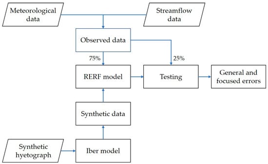
Figure 1.
Methodology scheme. The Regression-Enhanced Random Forest (RERF) model is used to build both models, only with observed data (RERF1) and with the combination of observed and synthetic data (RERF2).
- Rainfall and discharge data were collected from the meteorological and streamflow stations, respectively, to set every input and output of the models. This data set was further divided chronologically: 75% for training and 25% for testing (the most recent data).
- The numerical model based on Iber was calibrated, taking into account high events of the training set.
- Synthetic hyetographs with different periods of return were built using the Alternating Block Method (ABM) and intensity-duration-frequency (IDF) equations. They are employed in the calibrated Iber model to obtain synthetic hydrographs with higher streamflow values than those registered in the measured training set.
- Two RERF models were built using only the training data from the stations (RERF1) and a combination of the training set and the synthetic cases (RERF2).
- The testing set was evaluated considering both models, taking into account general errors and metrics focused on the most important values in the context of an imbalanced domain.
2.2. Study Area
The study area is the upper Fluvià river catchment, with the outlet point in Olot. The catchment is located in the autonomous community of Catalonia, Spain (Figure 2). It has an area of 133.68 km2, the mainstream length is approximately 22.60 km, the elevation ranging from 1547 to 397 masl, and the mean slope of the catchment is 34%. The concentration time computed by Témez [46] method is 3.9 h. The annual mean precipitation is 910 mm and the temperature varies from almost 40 °C in summer to −8 °C in winter. Within the catchment, there is only one meteorological station called la Vall d’en Bas operated by the Meteorological Service of Catalonia (Meteocat) and the streamflow gauge is located in the small town of Olot, in the outlet of the catchment, operated by the Catalan Water Agency (ACA).
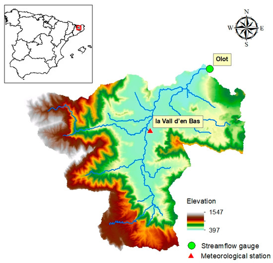
Figure 2.
Digital terrain model of Fluvià catchment based on the information of the Cartographic and Geological Institute of Catalonia (ICGC) [47].
According to the CORINE service [48], the catchment mainly comprises broad-leaved forest and arable lands with urban areas at the bottom. Based on information from the Cartographic and Geological Institute of Catalonia (ICGC) [47], udorthent lithic and hapludoll lithic are the principal soil formations in the region. Consequently, in the first layer, the presence of coarse and medium sand is predominant.
One of the main risks of the region is flash floods [49], which are the product of heavy rainfall in a short period of time. These rainfalls are mostly related to low-pressure nuclei reaching the Mediterranean after passing through Catalonia, advection processes from the east, and orographic influence [50]. According to Llasat [51], 82% of floods in Catalonia between 1982 and 2007 were flash floods, and the number of flood events has been increasing over recent years. In addition, the Olot municipality is cataloged as a high flood-risk area [52] by the Catalan administration. The last time that the river Fluvià overflowed on Olot city was in 2020 during the “Gloria” storm, where the total precipitation registered at la Vall d’en Bas station in four days reached 281.8 mm, representing roughly 30% of the total annual precipitation.
2.3. Data
Hourly rainfall from la Vall d’en Bas station and a 12-year discharge series from the Olot streamflow gauge, from 2010 to 2021, are used to set the inputs and outputs of the ML models. First, the time of prediction is selected based on the case of a possible application of an early warning system (EWS) for our model. Therefore, we took into consideration an acceptable time to warn the local population of a possible flood. In that sense, Rogers and Sorensen [53] and Aboelata et al. [54] mentioned that given an emergency, almost the entire population affected could be warned in approximately three hours. Hofflinger et al. [55] showed that for their flood event, around 80% of the people may be warned after 100 min. Consequently, three hours ahead was chosen as the prediction horizon.
Second, the input variables for the ML model are set based on the research done about the topic [41,56,57,58,59]. Hence, we considered past hourly precipitation (; ), past accumulated precipitation of T hours (; ), and past discharge in the streamflow gauge (. In all these variables, t represents the time of prediction, h and k refers to a time value in hours (e.g., means the discharge three hours before the time of prediction). Additionally, we also incorporated a discharge gradient between the discharges closest to the target (), as an attempt to represent future trends for the streamflow. In summary, our ML models follow Equation (1) to compute streamflow at time t:
A wide group of variables with different lag times was selected based on the possibility of the RERF algorithm to give more importance to some variables and constrain others internally. The RERF is an algorithm comprises two stages. In the first, the least absolute shrinkage and selection operator (Lasso) can reduce the influence of some variables and prioritize others in the regression [60]. In the second, the Random Forest (RF) algorithm predicts the residuals of Lasso and is based on decision tree structures where the corresponding partitions are created according to the variable that produces the most homogenous results [61]. Both stages contribute to selecting the variables with a higher influence on the model. A detailed explanation of the RERF algorithm is given in Section 2.6.
Finally, our models were trained using 75% (15 July 2010–8 August 2019) of the entire data, while 25% (8 August 2019–31 December 2021) were left for testing. The “Gloria” storm in 2020 was deliberately left in the testing set to evaluate the performance of the model on high streamflow values or even extrapolating, considering that this event generates the highest discharge in the data set. The missing values in our data set represent roughly 3% of the data; they being such small quantity, a filling process was not executed.
Figure 3a depicts the time series of both hourly precipitation and discharge. The highest values reach nearly 40 (mm) and 131 (m3/s) (Gloria storm), respectively. Very few discharge values are larger than 100 (m3/s), and, as said, the highest value was left in the testing set. Both streamflow and precipitation belong to an imbalance data set, with the highest values (the most relevant) being the great minority. For example, 1.2% of the streamflow data are larger or equal to 5.5 (m3/s), which represents the streamflow with one year of period of return and the median reaches 0.24 (m3/s), but the maximum is 131.36 (m3/s). This scenario is portrayed in Figure 3b,c through the density plots for precipitation and streamflow, respectively. Boxplots were built using the Medcouple function for skewed distributions [43].
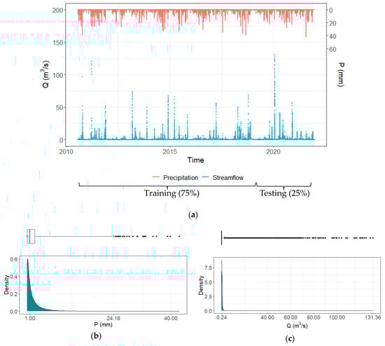
Figure 3.
(a) Time series plot of streamflow and precipitation; (b) density and boxplot for precipitation p > 0.1 (mm); (c) density and boxplot of streamflow.
2.4. Iber Model
This work employs the hydrological processes module of Iber (version 3.1) [62,63], a coupled hydrological-hydraulic distributed model that solves the rainfall-runoff process using the two-dimensional Shallow Water Equations based on the finite volume method [64,65]. Iber was developed in collaboration between the Mathematical Engineering Group (Universidade de Santiago de Compostela), the Water and Environmental Engineering Group (Universidade da Coruña), the Flumen Institute (Universitat Politècnica de Catalunya, and the International Centre for Numerical Methods in Engineering), and the Spanish National Public Works Research Centre (CEDEX), Spain [64]. The model employs a mesh (structured or unstructured) in two dimensions to discretize the catchment. This module takes into account precipitation (P) and losses (f) as new components of the mass conservation Equation (2) [62]:
where h is the water depth, and are the components of the unit discharge in x and y directions, respectively. To estimate the losses, several infiltration methods are included in the module. In this study, the SCS (Soil conservation Service) method was applied [66].
Consequently, the parameter considered in the calibration process was the curve number (CN). CN was computed as a weighted value regarding a simplified land use map based on CORINE data [48] and six land uses were adopted (Figure 4). The soil group selected was B, according to what was explained in Section 2.2. Considering this configuration, CN varies from 39 to 78 for dry to wet conditions, respectively. In the calibration process, CN = 45 was selected. Manning’s numbers for the different land use were left as default values given by the Iber model, which are taken from [67]. The wet-dry limit was set in 0.0001 (m) and the numerical scheme used was the decoupled hydrological discretization (DHD) [63].
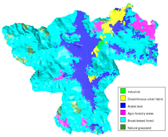
Figure 4.
Land use map from the Iber model. The mesh used in the Iber model has a size of 10 (m) at the riverbed and 300 (m) in the rest of the catchment.
2.5. Synthetic Cases
Synthetic hyetographs were built using the Alternating Block Method (ABM), which is a widely known method for designing precipitation hyetographs [66]. It consists of obtaining the intensities based on the IDF equation for different durations considering the total duration D = n·d, being n the number of time steps. Once the intensities have been computed, the precipitation depth is determined by . The difference between two consecutive precipitations corresponds to the precipitation depth of that time interval or block. The final synthetic hyetograph is obtained by ordering the blocks where the highest precipitation is located in the middle of the hyetograph and descending one block to the right and another to the left alternatively.
The IDF equation used for the ABM method was that of the la Vall d’en Bas station, determined following the methodology exposed in Aparicio Mijares [68] using 12 years of information. The equation is given by (3):
where i is the intensity (), T is the return period (years), and d is the duration (min); 34 h for the total duration of the rainfall was adopted based on the duration of the highest event of the training set (Q = 121 (m3/s)), considering the number of hours of registered precipitation (P > 0.1 (mm)) in the day of that event and the day before [69]. As period of return, 15, 20 and 25 years were selected for the IDF equation to obtain higher discharges than the ones in the training set.
2.6. Regression-Enhanced Random Forest (RERF)
Random Forest (RF) proposed by Breiman [70] is a widely used ML algorithm that has been applied in several streamflow prediction models [57,71]. However, one of the main limitations of this algorithm is its lack of suitable predictions when the outputs are beyond the values used in the training set [72]. To overcome this limitation, Zhang et al. [24] proposed RERF, which combines Lasso regression with RF.
The least absolute shrinkage and selection operator (Lasso) technique proposed by Tibshirani [60] is a parametric regression that minimizes the expression given by (4) applying a penalization function , which is equal to the absolute value of the coefficients :
where are the inputs of the regression, are the outputs, p is the number of features, and λ is a penalization parameter that must be tuned according to a cross-validation procedure. This method tends to shrink or reduce the coefficients () to 0 even some of the coefficients may be 0. Therefore, it is also used in variable selection procedures because it discards some of the variables that do not add information to the model.
In contrast to Lasso, RF is a nonparametric method based on an ensemble of decision trees. The method starts with an allocation function that combines a random selection of the inputs and a technique called bagging, which creates different data sets based on bootstrap sampling [73]. This technique repeats some examples and takes out others (out-of-bag data). Decision trees are applied to the different data sets and in the case of regression models, the prediction is made by the average of the predictions of the trees in the model. RF is a robust method that tends to avoid overfitting [74]. The required steps to develop an RERF method are:
- The k-fold cross-validation method with 10-folds is applied using Lasso regression and the training set following Equation (1) to obtain a suitable penalization parameter (λ). After that, the Lasso model is trained considering the determined λ and the entire training set to establish the coefficients of Equation (5):where Y is the set of outputs (observed streamflow at time t), X is the set of inputs, and βλ are the Lasso coefficients. This study uses the R package glmnet (version 4.1-7) [75] to train the Lasso model.
- 2.
- An RF model is built using the same inputs given in (1) and the error from the Lasso regression (ϵλ) as the output according to (6):The RF model uses the default parameters for the number of trees (ntree) and the number of features (mtry) from the randomForest package of R language [76] and it is denoted by Tntree,mtry (X).
- 3.
- Finally, the RERF model is given by the sum of the Lasso and the RF model (7). In this sense, according to Zhang et al. [24], it is possible to find linear relations between the inputs and the output, making an approximated extrapolation possible.
2.7. General and Focused Errors
Regression models are usually evaluated employing general metrics such as mean absolute error (MAE), root mean squared error (RMSE), mean absolute percentage error (MAPE) and coefficient of determination (R2), among others [39,77,78]. These metrics consider the whole data set to be equally relevant when they are applied to the whole dataset. This is not our case, as the most valuable predictions correspond to high streamflow values related to flood events. However, the overwhelming majority of our data set is composed of low or base streamflow. Therefore, this study proposes the use of error metrics focused on estimating the performance of the model under imbalance domain conditions. The ultimate goal is to have a suitable measure of prediction capabilities regarding the most relevant values in practice. To compare the general (applied to the whole data set) and focused errors, both are computed. The general errors considered in this study are MAE, RMSE, MAPE and R2, they are given by:
where n is the total number of data, and are the predicted and observed streamflow, respectively, and are the mean values of predicted and observed streamflow, respectively. MAE, RMSE and MAPE are precision metrics of the model and they vary from 0 to ∞, where values close to 0 indicate high precision of the predictions. is a dispersion measurement, which varies from 0 to 1, indicating the lowest and the highest correlation between observed and predicted values, respectively [79]. The focused errors of this study are divided into scalar, graphical-based errors [80] and errors by event. In Figure 5, a summary of these and their structure is shown, while the different errors are described in subsequent sections.
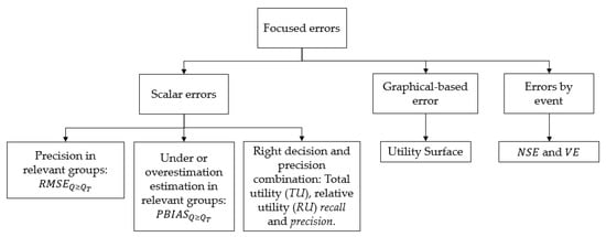
Figure 5.
Structure of the focused errors used in this study.
As mentioned in Section 2.3, a small proportion of the data are high streamflow values, but they are the most relevant for our purposes considering that these models are intended to be used on EWS. In that sense, this study evaluates the performance of the model focused on this group of data to obtain a more accurate picture of the model capabilities under these conditions and to avoid the influence of the great quantity of small streamflow values in the error metrics. To define the relevant groups, the bankfull flow is adopted. This value has been related to streamflow with return period from one to two years [81,82]. Therefore, in this study, , , and are employed to establish the relevant groups (), the last one with a special approach to the highest streamflow values.
In order to find the streamflow values for a certain return period, we took into consideration 24 yearly maximum streamflow values that were at our disposal (from 1996 to 2008 and from 2011 to 2021). Years with most of the data complete were considered. These data were adjusted to a generalized extreme value distribution type I (GEV I) (Figure 6), which has been widely employed for frequency analysis in the field of hydrology [66,83]. However, to test whether the distribution generates an acceptable adjustment, the Kolmogorov-Smirnov test was applied. It resulted in an acceptable adjustment for a 0.05 significance level (). Based on the theoretical distribution, , , and .
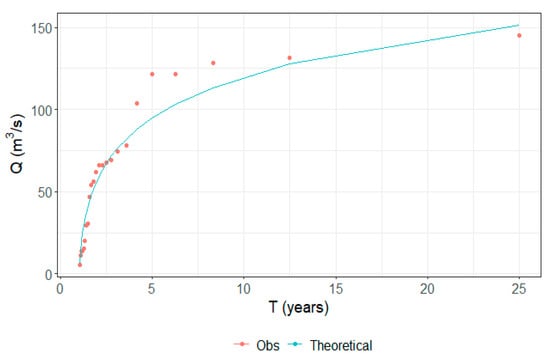
Figure 6.
GEV I distribution of peak streamflow.
2.7.1. Scalar Errors
The first purpose of performance evaluation is to measure precision. In our case, RMSE is used for the different relevant groups . Another aspect that must be taken into account is overestimation and underestimation. In the context of flooding prediction, overestimation can lead to a false alarm, which is related to some costs, such as the interruption of highways and streets or several activities in the involved area. However, underestimation may lead to great material and human losses that, in the last case, are unmeasurable moneywise [82]. Consequently, a model with less underestimation is more suitable for our purposes. To estimate that, the percentage bias corresponding to the relevant groups (), Equation (12) was employed:
where and are the observed and predicted streamflow inside relevant groups, respectively. If PBIAS is larger than 0, the model overestimates, while smaller values denote underestimation [84].
If an inaccurate prediction is made, but this prediction leads to the right action (e.g., issue an alarm), it has a value, i.e., a benefit. On the other hand, if the prediction leads to the wrong action (false alarm or missing alarm), the prediction is costly. Based on this idea, the utility of a prediction can be estimated. Our analysis is based on the work of Ribeiro [85] to evaluate the benefits, costs and, ultimately, the utility. In Equation (13), we must consider that the costs are always negative, according to the aforementioned work:
where U is the utility, B are the benefits, and C are the costs. In order to define the utility of a prediction, a relevant function is established to identify the importance of every prediction. Consequently, in Figure 7, this function is defined taking into account as control points the streamflow values for T = 1 and T = 1.5 ( and , respectively).
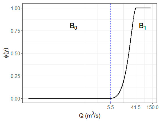
Figure 7.
Relevance function of streamflow.
The relevance function ( [0, 1] was built using the Piecewise Cubic Hermite Interpolating Polynomials function (pchip), as it was suggested by Ribeiro [85], using the library pracma of R programming language [86]. The subgroups (also called bumps) and represent two different actions, not to issue an alarm and issue it, respectively. Values below 5.5 (m3/s) () do not have relevance because they are so small that there is no need to issue an alarm by flooding. From 5.5 (m3/s) onwards (), the relevance starts to grow until it reaches the maximum value at 41.5 (m3/s), and from there, the relevance is the highest for every value. If the observed and predicted values do not have relevance, there is no utility.
The predicted value must fulfill two conditions to carry some benefit: (1) it must allow us to take the right action (if the prediction corresponds to another bump, there is no benefit because it leads to the wrong action), and (2) it must have an acceptable precision. The benefit of the prediction () is given by (14):
The maximum possible benefit (MPB) corresponds to the relevance value of the observed streamflow, . Hence, if the observed value is smaller than 5.5 (m3/s), there is no benefit. is a function that computes the fraction of MPB that can be obtained as a result of the prediction. In Appendix A, the equations leading to the computation of are developed in detail according to Ribeiro [85].
Analogously, the cost of a predicted value () depends on (1) whether it leads to the wrong action and (2) the inaccuracy of the prediction. Contrary to the benefits, where only the relevance of the observed value is considered, in this case, the relevance of the predicted value is also taken into account because taking the wrong action comes with a cost (although it does not involve a benefit). Therefore, a joint relevance function () that weights both observed and predicted relevance is adopted (15). The relevance function of the predicted values ()) is also described as in Figure 7. Finally, is described by (16):
where p is parameter [0, 1], which weights the relevance of the observed and predicted values. We adopted p = 0.6, which gives higher importance to the observed relevance value. plays the same role as , being the fraction of the joint relevance function taken as a cost. The calculation of is explained in Appendix B. Once the benefit and cost of every prediction have been computed, Equation (13) is applied to obtain the utility. The total utility (TU) for the model is given by Equation (17):
where is the utility as a result of the prediction of individual predictions [−1, 1]. If either the predicted () or the observed value () belong to , there is a utility different than 0 related to these values.
The maximum utility is achieved when there are no costs () and the maximum benefit has been obtained. In this situation, the maximum benefit is given by the value of the relevance function for the observed value (). Hence, to estimate the fraction of the maximum utility that the model has reached, the relative utility (RU) is also added to the analysis and is given by (18):
To evaluate if the model reaches the maximum possible utility for a given observation and prediction, Branco [80] developed an adaptation of recall (19) and precision (20) for regression models as a function of utility. Therefore, from this analysis, recall is the proportion of the maximum utility achieved due to positive observations. Precision refers to the fraction of utility achieved due to positive predictions. To label observations and predictions as positive (belonging to a class or interval), Branco [80] uses a threshold of the relevance function, (e.g., or ). In our analysis, the maximum relevance () was adopted; this value corresponds to . Consequently, recall and precision are given by:
2.7.2. Graphical-Based Errors
Graphical-based errors (GBE) are designed to give a meticulous image of certain aspects of the model performance. This study employs the utility surface for regression models [85], which is based on the interpolation of the individual utility values of every prediction. The inverse distance weighted (IDW) method is applied for utility interpolation. The IDW power of four was adopted to stress the influence of the nearest point [87] and to make the different utility values more distinguishable. The coordinates of the surface are the observed and predicted values. The GBE makes it simple to identify where the utility reaches the highest values or the cost generates negative values highlighting the model performance regarding the relevant data.
2.7.3. Errors by Event
In the context of an imbalanced domain, it is possible that several inaccurate predictions in relevant groups come from a single event. Therefore, in order to assess this situation and the model performance under time variation, the evaluation by event has been incorporated. One of the most widely used performance measures for hydrological models is Nash-Sutcliffe Efficiency (NSE) [88] given by (21), although some authors have discussed its suitability because it is overinfluenced by high values due to the squared terms [79]. To avoid this misjudgement, volume efficiency (VE) [89] was added to the analysis and it is given by (22):
This metric measures the proportion of the observed volume of water that is delivered as a result of the prediction in a specific timeframe, varying from 1 for maximum similarity to 0 for a poor model.
3. Results and Discussion
3.1. Synthetic Cases
Three events of the training set were used to calibrate the Iber model for the catchment (Figure 8). They were selected because they are among the highest events in the training set. Figure 8a shows the highest events in the training set and the Iber model results. The peak discharge is 121 (m3/s) and the timeframe considered was from 14 March 2011 to 16 March 2011. Figure 8b,c shows two of the highest events of the training set with peak discharges of 74.3 and 67.7 (m3/s), respectively. The timeframes considered for these events are from 4 March 2013 to 7 March 2013 and from 27 November 2014 to 2 December 2014, respectively. NSE reached was either good or satisfactory according to the bibliography [90,91], with values of 0.64 (Figure 8a), 0.67, and 0.37 (Figure 8b,c) for the three events, respectively.
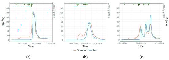
Figure 8.
Calibration events for the Iber model: (a) Highest event of training set; (b,c) second and third event for calibration, respectively. The green bars represent the hyetographs of the events.
Once the model was calibrated, synthetic hydrographs were generated employing the synthetic hyetographs obtained with the ABM method (Section 2.5). Figure 9 depicts the synthetic hyetographs and the respective hydrographs as a result of their application to the calibrated Iber model. The hydrographs reached 141.19, 190.33, and 233.29 (m3/s). All of them are higher than the maximum streamflow registered in the training set (121 (m3/s)) whereby they are aimed at improving the prediction performance over high discharge values of the ML model. The synthetic data generated in this way are added to the training set according to the respective inputs for the model.
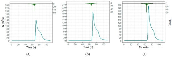
Figure 9.
Synthetic hydrographs generated with the calibrated Iber model: (a) T = 15 years, (b) T = 20 years, (c) T = 25 years. The green bars represent the synthetic hyetograph.
3.2. General Errors
The model built with only observed data from the stations is called RERF1, and the model trained with the combination of observed and synthetic data is called RERF2. The following results are a consequence of the application of these models to the testing set. As previously mentioned, the Gloria storm in 2020 represents the highest event registered in the data set and it has been left as part of the testing set to evaluate the ML model capabilities in the most relevant data.
Figure 10 shows the scatter plot of both models, with an ideal tendency in blue. The highlighted points belong to the Gloria storm. All values higher than 60 (m3/s) belong to this storm. There are simple identified differences between the two plots, showing how several points are closer to the ideal line for RERF2, especially on high values. Apparently, this model has better performance. Nonetheless, this is not clearly depicted in the general error metrics (Table 1).
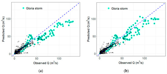
Figure 10.
Scatter plot of the testing set. (a) RERF1, (b) RERF2. The blue line represents the ideal prediction. The highlighted points are Gloria storm data.

Table 1.
General errors of the testing set for RERF1 and RERF2 models.
The predictions of both models acceptably capture the dispersion of the observations, which are depicted in values close to 1, although this metric does not reflect the apparent improvement of RERF2 concerning high values. The differences between models regarding MAE and MAPE are minimal, while RMSE is 14% lower for RERF2. This shows that the greatest differences are obtained for higher flows (RMSE penalizes large errors more than MAE). However, these values do not give an accurate indication of the performance of the model under high streamflow. The overwhelming majority of the data correspond to low values and, therefore, is not relevant in the context of this work.
3.3. Focused Errors
When we evaluate the models focusing on relevant ranges (, the difference in performance between models becomes apparent. The scalar errors are depicted in Table 2, where RERF2 model outperformed the RERF1 model in every metric. The precision measured by RMSE has increased, reaching the highest improvement at , where the most relevant streamflow values are located. Both models tend to underestimate high values. However, such a tendency is considerably reduced in RERF2, representing an improvement of up to 38.71%.
Table 2.
Scalar errors for the testing set.
RERF2 also shows better performance considering the combination of the right action prediction and precision. This is portrayed in the difference in TU between the models, with an increase of 10.56% for RERF2. Both models reach more than half of the maximum possible utility, represented in relative utility terms (0.53 and 0.58, respectively). The total utility obtained from the predictions and observations higher than also increased for RERF2 by more than 10%, as reflected in precision and recall metrics. In other words, RERF2 obtains a mean of 0.80 of the maximum utility for prediction over and 0.77 for observations with the same criterion.
Utility increases in the high ranges when we compare RERF1 and RERF2 under the utility surface analysis (Figure 11 and Figure 12), even reaching peaks of utility close to 1 in RERF2 for values over 70 (m3/s). This is not the case for RERF1, where the maximum utility is close to 0.7 for these ranges. For values over 100 (m3/s), the improvement is less accentuated. Nonetheless, it exists and is reflected in the presence of negative utility in RERF1 (cost higher than benefits) for the prediction of the highest observed streamflow, which does not happen in RERF2.
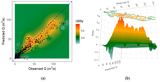
Figure 11.
Utility surface of the testing set for RERF1. (a) 2D plot; (b) 3D plot. The blue line represents the ideal prediction.
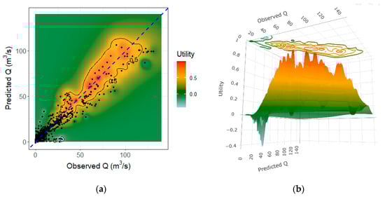
Figure 12.
Utility surface of the testing set for RERF2. (a) 2D plot; (b) 3D plot. The blue line represents the ideal prediction.
To evaluate the performance of the models under specific events, three storms were selected. They produced the highest streamflow in the testing set and composed the majority of points inside the relevant groups. The first of these events corresponds to the Gloria storm and is depicted in Figure 13.
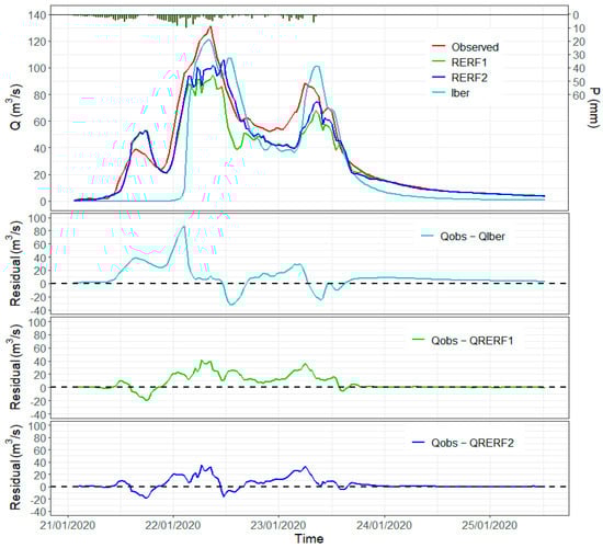
Figure 13.
Gloria storm hydrograph with observed values, RERF1, RERF2, and Iber model results. Residuals for the models with respect to the observed values are also depicted.
RERF1 and RERF2 show acceptable performance for the Gloria storm, as can also be verified in Table 3, showing NSE and VE coefficients higher than 0.75 for both models. Nonetheless, there is an improvement of more than 6% in both metrics of RERF2 with respect to RERF1. This improvement takes place in the peaks of the hydrograph of the Gloria storm and its falling limbs (Figure 13), which is specially appreciated close to 22 January 2020 12:00, where the residuals of RERF2 with respect to the observed values are considerably smaller than the ones produced for RERF1. After that, there is a period where RERF1 and RERF2 overlap each other (around 23 January 2020 0:00) to finally reach the last peak of the storm (close to 23 January 2020 12:00), where there is also a considerable difference between models again. The Iber model results were added to Figure 13 because they reach higher values than the ML models in the periods where RERF2 obtains more accurate results than RERF1. This suggests that RERF2 was able to improve its performance in high ranges due to the synthetic Iber cases (higher than the observed) added to the training set.
Table 3.
NSE and VE by event for RERF1 and RERF2.
The hydrographs of RERF1 and RERF2 for the Gloria storm present a brief period of noise at the highest discharges of the event (Figure 13). They match the precipitation variation in the hyetograph (short periods of time where the precipitation increases and decreases, generating small peaks). In the highest ranges, the ML models were not able to fully capture the tendency of the observed hydrograph. This situation might be due to the lack of data at these ranges and to the different shapes of the synthetic hyetograph and the real ones (we used a smooth distribution of the precipitation), from where RERF2 could gain information. It must also be taken into account that in the synthetic models, the precipitation is assumed to be homogeneous over the entire catchment area. This is an approximation of reality and may introduce a relevant error in some cases. In particular, the irregular evolution of hourly precipitation in the early hours of 22 January 2020 may not represent the actual average value for the area. Additional precipitation information in other places of the catchment might improve the model, avoiding this kind of tendency disruption. Nonetheless, it should be mentioned that the Iber model is not affected by this issue (streamflow results are smoother). In the second and third events selected from the testing set (Figure 14a,b), the models also exhibit suitable performance. Although there are small differences between metrics, the models perform almost equally. Synthetic data do not have a considerable impact on small events (<60 (m3/s)).
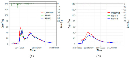
Figure 14.
(a) Second-highest event in the testing set; (b) third-highest event in the testing set.
3.4. Overall Discussion
The proposed methodology is based on the notion of relevant values and the imbalanced domain of streamflow records. Therefore, the addition of synthetic information is made in the most relevant group (high values for EWS applications). In this sense, the combination of synthetic and observed data to train an RERF model is able to enhance the prediction accuracy of high streamflow values with respect to an RERF model solely trained with observed data. Considerable improvements can be appreciated, especially in streamflow values larger than three years of return period. However, the results indicate that the methodology might be further improved with the addition of synthetic hyetographs with a time distribution similar to the observed ones. This might help improve the predicted shape of the hydrographs.
Similar results of evaluation metrics have been shown in the related literature regarding general errors. Cho and Kim [31] achieved correlation coefficients (R) of 0.98 and NSE of 0.95 for their daily model, which combined a physically based and an LSTM model. Konapala et al. [32] also showed NSE values larger than 0.75 for a considerable number of catchments in their study, where the models that combine physically based and ML models achieved more accurate results than model purely physically based models. Xie et al. [29] depicted mean NSE values of 0.61 for a large group of catchments and physically constrained ML models. Snieder et al. [44] defined values higher than the 80th percentile as high flow. The maximum NSE for the group with high values in this study is 0.72. An NSE value of 0.94 was obtained by Lin et al. [41] for values higher than 400 (m3/s) (the highest discharges in their study) with a prediction model one hour ahead. These results presented in the literature are consistent with the of the whole data set and the NSE values for Gloria Storm and the other events of the testing set developed in the present study.
Yang et al. [39] compared ML and physically guided ML models and determined that the incorporation of physically guided information helped to increase the NSE coefficient by 23% of the ML model. Furthermore, the underestimation also reduced due to this combination. This aspect corresponds with the results exposed in the present study, where the NSE of RERF2 improves for Gloria storm with respect to RERF1 and the PBIAS for the different ranges ( and ) is considerably reduced. Hourly predictions for typhon events were generated by Young et al. [36], where their combined model that uses HEC-HMS output as inputs of the ML model reached enhancements larger than 20% in RMSE compared to purely ML models. This is consistent with the RMSE improvement of RERF2 with respect to RERF1 for discharges higher than .
Utility analysis does not make a division by range to evaluate the predictions; instead, it separates the whole data set of both predictions and observations according to a relevance function. In this sense, it is able to suitably identify the benefits and costs of all the predictions, highlighting the ones with the highest utility for our purposes. Either numerically or graphically, the utility can express the improvement of a model due to more accurate predictions of relevant values (high streamflow). To the best of our knowledge, the utility measurements shown in this study have not been part of other evaluation analyses of streamflow prediction models using combined physically based and ML models. In that sense, it was not possible to compare the results of similar studies.
4. Conclusions
Streamflow prediction models intended to be used in early warning systems for flooding are focused on high discharges. However, the streamflow records are heterogenous, and high discharges compose a small part of the data, although they are the most relevant. Therefore, evaluating the performance of streamflow prediction models under general metrics that take all the data into account is not a suitable approach because, being so scarce the relevant values, the prediction capabilities of these values are neither identifiable nor suitably measurable. Error metrics focused on relevant values are a more useful approach. This study employs observed discharge over a certain period of return ( to define relevant groups.
The addition of synthetic streamflow data generated by a physical model (Iber) and synthetic precipitation built with the ABM method to the observed training set contributes to improving the performance of the ML model over relevant groups (high streamflow values) compared to the ML model that is only trained with observed data. The peak discharges of synthetic data are higher than the maximum observed events in the training and the contribution of this information is reflected in the improvement of the performance of the ML model on the highest streamflow values.
The precision of the model that combines synthetic and observed data in the training set (RERF2) with respect to the one that only considers observed data (RERF1) has increased, with lower RMSE values on relevant groups (especially in ) for RERF2 than for RERF1. The same can be seen on a higher NSE and VE for the largest event of the testing set (Gloria storm) for RERF2 than for RERF1. RERF2 also shows a reduction in the underestimation for relevant groups with respect to RERF1 (low values).
Further analysis was made based on the utility concept, which measures the capability of the model to predict the right action to take (issue an alarm or not), combined with the precision of the prediction. This analysis measures whether the prediction carries out a benefit or a cost and characterizes predictions and observations using a relevance function. In this sense, it is a more robust analysis than the one given by the metrics mentioned above because the relevance of both observations and predictions are estimated instead of metrics that only consider if the observed value belongs to a relevant group. Predictions of the RERF2 model present higher utility than the ones from RERF1, this is especially achieved in the highest streamflow values of the testing set and, therefore, the most relevant.
In general terms, the utility from predictions and the possible utility due to observations greater than are larger for RERF2 than for RERF1, as portrayed in the increase of precision and recall, respectively. Therefore, RERF2 is not only more accurate, but also can predict the right action in a proper way.
The addition of synthetic data has almost no impact on small ranges (lower than ). Therefore, the accuracy under these ranges has not been compromised by the addition of synthetic information. The results suggest that the incorporation of synthetic events created with different hyetographs with similar shapes to the observed ones might contribute to improving the capture of the shape of the hydrographs in the highest streamflow values.
Streamflow prediction models for EWS may be improved based on this methodology, where accuracy over high values is crucial. Valuable and reliable information about possible upcoming hazardous streamflow values might be given to emergency services to take the respective measures. Future applications that increase the lead time can help increase the effectiveness of the actions taken by these services.
Author Contributions
Conceptualization, S.R.L.-C., F.S. and E.B.; methodology, S.R.L.-C., F.S. and E.B.; software, S.R.L.-C., validation, S.R.L.-C.; formal analysis, S.R.L.-C.; investigation, S.R.L.-C.; data curation, S.R.L.-C.; writing—original draft preparation, S.R.L.-C.; writing—review and editing, S.R.L.-C., F.S. and E.B.; visualization, S.R.L.-C.; funding acquisition, F.S. and E.B. All authors have read and agreed to the published version of the manuscript.
Funding
This work was funded by the Grants PID2021-122661OB-I00 funded by MCIN/AEI/ 10.13039/501100011033 and “ERDF A way of making Europe”, TED2021-129969B-C33 funded by MCIN/AEI/ 10.13039/501100011033 and the “European Union NextGenerationEU/PRTR”, CEX2018-000797-S funded by MCIN/AEI /10.13039/501100011033, and the Generalitat de Catalunya through the CERCA Program.
Data Availability Statement
The data regarding this research are available on request to the authors, the Meteorological Service of Catalonia (Meteocat) and the Catalan Water Agency (ACA).
Conflicts of Interest
The authors declare no conflict of interest.
Appendix A
Following the methodology depicted by Ribeiro [85], the computation of the bounded loss function is given by the following steps:
The limits of the bumps are defined, and . Figure A1 shows where these limits are located. In our case, , , , and . Depending on the value of the observed data, , takes values of 0, 1 or 2.

Figure A1.
Theoretical relevance function for streamflow prediction analysis.
Figure A1.
Theoretical relevance function for streamflow prediction analysis.

The benefit threshold ( is computed according to (A1), where is the maximum admissible loss (A2). is given by (A3).
If is located in the bump, , , , and .
is the absolute deviation between prediction and observation (A4).
Finally, the bounded loss function is given by:
Appendix B
is the bounded loss function used to compute costs. We followed the same methodology developed in Appendix A to calculate , with the following main two differences given by (A6) and (A7).
References
- Stefanidis, S.; Stathis, D. Assessment of Flood Hazard Based on Natural and Anthropogenic Factors Using Analytic Hierarchy Process (AHP). Nat. Hazards 2013, 68, 569–585. [Google Scholar] [CrossRef]
- UNISDR. Global Assessment Report on Disaster Risk Reduction; United Nations: Geneva, Switzerland, 2015; ISBN 9789211320428. [Google Scholar]
- Jongman, B.; Kreibich, H.; Apel, H.; Barredo, J.I.; Bates, P.D.; Feyen, L.; Gericke, A.; Neal, J.; Aerts, J.C.J.H.; Ward, P.J. Comparative Flood Damage Model Assessment: Towards a European Approach. Nat. Hazards Earth Syst. Sci. 2012, 12, 3733–3752. [Google Scholar] [CrossRef]
- Laudan, J.; Zöller, G.; Thieken, A.H. Flash Floods versus River Floods-a Comparison of Psychological Impacts and Implications for Precautionary Behaviour. Nat. Hazards Earth Syst. Sci. 2020, 20, 999–1023. [Google Scholar] [CrossRef]
- Hapuarachchi, H.A.P.; Wang, Q.J.; Pagano, T.C. A Review of Advances in Flash Flood Forecasting. Hydrol. Process. 2011, 25, 2771–2784. [Google Scholar] [CrossRef]
- Kobiyama, M.; Goerl, R.F. Quantitative Method to Distinguish Flood and Flash Flood as Disasters. SUISUI Hydrol. Res. Lett. 2007, 1, 11–14. [Google Scholar] [CrossRef]
- Kundzewicz, Z.W.; Kanae, S.; Seneviratne, S.I.; Handmer, J.; Nicholls, N.; Peduzzi, P.; Mechler, R.; Bouwer, L.M.; Arnell, N.; Mach, K.; et al. Flood Risk and Climate Change: Global and Regional Perspectives. Hydrol. Sci. J. 2014, 59, 1–28. [Google Scholar] [CrossRef]
- Zanchetta, A.D.L.; Coulibaly, P. Hybrid Surrogate Model for Timely Prediction of Flash Flood Inundation Maps Caused by Rapid River Overflow. Forecasting 2022, 4, 126–148. [Google Scholar] [CrossRef]
- Cools, J.; Innocenti, D.; O’Brien, S. Lessons from Flood Early Warning Systems. Environ. Sci. Policy 2016, 58, 117–122. [Google Scholar] [CrossRef]
- Giannaros, C.; Dafis, S.; Stefanidis, S.; Giannaros, T.M.; Koletsis, I.; Oikonomou, C. Hydrometeorological Analysis of a Flash Flood Event in an Ungauged Mediterranean Watershed under an Operational Forecasting and Monitoring Context. Meteorol. Appl. 2022, 29, e2079. [Google Scholar] [CrossRef]
- Casagrande, L.; Tomasella, J.; dos Santos Alvalá, R.C.; Bottino, M.J.; de Oliveira Caram, R. Early Flood Warning in the Itajaí-Açu River Basin Using Numerical Weather Forecasting and Hydrological Modeling. Nat. Hazards 2017, 88, 741–757. [Google Scholar] [CrossRef]
- Mosavi, A.; Ozturk, P.; Chau, K.W. Flood Prediction Using Machine Learning Models: Literature Review. Water 2018, 10, 1536. [Google Scholar] [CrossRef]
- Bourdin, D.R.; Fleming, S.W.; Stull, R.B. Streamflow Modelling: A Primer on Applications, Approaches and Challenges. Atmosphere-Ocean 2012, 50, 507–536. [Google Scholar] [CrossRef]
- Majone, B.; Avesani, D.; Zulian, P.; Fiori, A.; Bellin, A. Analysis of High Streamflow Extremes in Climate Change Studies: How Do We Calibrate Hydrological Models? Hydrol. Earth Syst. Sci. 2022, 26, 3863–3883. [Google Scholar] [CrossRef]
- Huang, X.; Li, Y.; Tian, Z.; Ye, Q.; Ke, Q.; Fan, D.; Mao, G.; Chen, A.; Liu, J. Evaluation of Short-Term Streamflow Prediction Methods in Urban River Basins. Phys. Chem. Earth 2021, 123, 103027. [Google Scholar] [CrossRef]
- Kratzert, F.; Klotz, D.; Shalev, G.; Klambauer, G.; Hochreiter, S.; Nearing, G. Benchmarking a Catchment-Aware Long Short-Term Memory Network (LSTM) for Large-Scale Hydrological Modeling. Hydrol. Earth Syst. Sci. Discuss. 2019, 2019, 1–32. [Google Scholar] [CrossRef]
- Jehanzaib, M.; Ajmal, M.; Achite, M.; Kim, T.W. Comprehensive Review: Advancements in Rainfall-Runoff Modelling for Flood Mitigation. Climate 2022, 10, 147. [Google Scholar] [CrossRef]
- Di Nunno, F.; de Marinis, G.; Granata, F. Short-Term Forecasts of Streamflow in the UK Based on a Novel Hybrid Artificial Intelligence Algorithm. Sci. Rep. 2023, 13, 7036. [Google Scholar] [CrossRef]
- Kratzert, F.; Klotz, D.; Herrnegger, M.; Hochreiter, S. A Glimpse into the Unobserved: Runoff Simulation for Ungauged Catchments with LSTMs. In Workshop on Modelling and Decision-Making in the Spatiotemporal Domain, 32nd Conference on Neural Information Processing Systems; NeuRIPS: Montréal, QC, Canada, 2018; Available online: http://www.openreview.net/forum?id=Bylhm72oKX (accessed on 20 February 2023).
- Kim, T.; Yang, T.; Gao, S.; Zhang, L.; Ding, Z.; Wen, X.; Gourley, J.J.; Hong, Y. Can Artificial Intelligence and Data-Driven Machine Learning Models Match or Even Replace Process-Driven Hydrologic Models for Streamflow Simulation?: A Case Study of Four Watersheds with Different Hydro-Climatic Regions across the CONUS. J. Hydrol. 2021, 598, 126423. [Google Scholar] [CrossRef]
- Gauch, M.; Mai, J.; Gharari, S.; Lin, J. Data-Driven vs. Physically-Based Streamflow Prediction Models. In Proceedings of the 9th International Workshop on Climate Informatics, Paris, France, 2–4 October 2019. [Google Scholar]
- Bhasme, P.; Vagadiya, J.; Bhatia, U. Enhancing Predictive Skills in Physically-Consistent Way: Physics Informed Machine Learning for Hydrological Processes. J. Hydrol. 2022, 615, 128618. [Google Scholar] [CrossRef]
- Duan, S.; Ullrich, P.; Shu, L. Using Convolutional Neural Networks for Streamflow Projection in California. Front. Water 2020, 2, 28. [Google Scholar] [CrossRef]
- Zhang, H.; Nettleton, D.; Zhu, Z. Regression-Enhanced Random Forests. arXiv 2019, arXiv:1904.10416v1. [Google Scholar]
- Slater, L.J.; Arnal, L.; Boucher, M.-A.; Chang, A.Y.-Y.; Moulds, S.; Murphy, C.; Nearing, G.; Shalev, G.; Shen, C.; Speight, L.; et al. Hybrid Forecasting: Blending Climate Predictions with AI Models. Hydrol. Earth Syst. Sci. 2023, 27, 1865–1889. [Google Scholar] [CrossRef]
- Wi, S.; Steinschneider, S. Assessing the Physical Realism of Deep Learning Hydrologic Model Projections Under Climate Change. Water Resour. Res. 2022, 58, e2022WR032123. [Google Scholar] [CrossRef]
- Khandelwal, A.; Xu, S.; Li, X.; Jia, X.; Stienbach, M.; Duffy, C.; Nieber, J.; Kumar, V. Physics Guided Machine Learning Methods for Hydrology. arXiv 2020, arXiv:2012.02854v1. [Google Scholar]
- Hoedt, P.-J.; Kratzert, F.; Klotz, D.; Halmich, C.; Holzleitner, M.; Nearing, G.; Hochreiter, S.; Klambauer, G. MC-LSTM: Mass-Conserving LSTM. In Proceedings of the 38th International Conference on Machine Learning, Virtual, 18–24 July 2021. [Google Scholar]
- Xie, K.; Liu, P.; Zhang, J.; Han, D.; Wang, G.; Shen, C. Physics-Guided Deep Learning for Rainfall-Runoff Modeling by Considering Extreme Events and Monotonic Relationships. J. Hydrol. 2021, 603, 127043. [Google Scholar] [CrossRef]
- Asadieh, B.; Krakauer, N.Y. Global Change in Streamflow Extremes under Climate Change over the 21st Century. Hydrol. Earth Syst. Sci. 2017, 21, 5863–5874. [Google Scholar] [CrossRef]
- Cho, K.; Kim, Y. Improving Streamflow Prediction in the WRF-Hydro Model with LSTM Networks. J. Hydrol. 2022, 605, 127297. [Google Scholar] [CrossRef]
- Konapala, G.; Kao, S.C.; Painter, S.L.; Lu, D. Machine Learning Assisted Hybrid Models Can Improve Streamflow Simulation in Diverse Catchments across the Conterminous US. Environ. Res. Lett. 2020, 15, 104022. [Google Scholar] [CrossRef]
- Abebe, A.J.; Price, R.K. Managing Uncertainty in Hydrological Models Using Complementary Models. Hydrol. Sci. J. 2003, 48, 679–692. [Google Scholar] [CrossRef]
- Lu, D.; Konapala, G.; Painter, S.L.; Kao, S.C.; Gangrade, S. Streamflow Simulation in Data-Scarce Basins Using Bayesian and Physics-Informed Machine Learning Models. J. Hydrometeorol. 2021, 22, 1421–1438. [Google Scholar] [CrossRef]
- Liu, B.; Tang, Q.; Zhao, G.; Gao, L.; Shen, C.; Pan, B. Physics-Guided Long Short-Term Memory Network for Streamflow and Flood Simulations in the Lancang–Mekong River Basin. Water 2022, 14, 1429. [Google Scholar] [CrossRef]
- Young, C.C.; Liu, W.C.; Wu, M.C. A Physically Based and Machine Learning Hybrid Approach for Accurate Rainfall-Runoff Modeling during Extreme Typhoon Events. Appl. Soft Comput. J. 2017, 53, 205–216. [Google Scholar] [CrossRef]
- Liu, J.; Yuan, X.; Zeng, J.; Jiao, Y.; Li, Y.; Zhong, L.; Yao, L. Ensemble Streamflow Forecasting over a Cascade Reservoir Catchment with Integrated Hydrometeorological Modeling and Machine Learning. Hydrol. Earth Syst. Sci. 2022, 26, 265–278. [Google Scholar] [CrossRef]
- Mohammadi, B.; Moazenzadeh, R.; Christian, K.; Duan, Z. Improving Streamflow Simulation by Combining Hydrological Process-Driven and Artificial Intelligence-Based Models. Environ. Sci. Pollut. Res. 2021, 28, 65752–65768. [Google Scholar] [CrossRef] [PubMed]
- Yang, S.; Yang, D.; Chen, J.; Santisirisomboon, J.; Lu, W.; Zhao, B. A Physical Process and Machine Learning Combined Hydrological Model for Daily Streamflow Simulations of Large Watersheds with Limited Observation Data. J. Hydrol. 2020, 590, 125206. [Google Scholar] [CrossRef]
- Feng, D.; Lawson, K.; Shen, C. Mitigating Prediction Error of Deep Learning Streamflow Models in Large Data-Sparse Regions with Ensemble Modeling and Soft Data. Geophys. Res. Lett. 2021, 48, e2021GL092999. [Google Scholar] [CrossRef]
- Lin, Y.; Wang, D.; Wang, G.; Qiu, J.; Long, K.; Du, Y.; Xie, H.; Wei, Z.; Shangguan, W.; Dai, Y. A Hybrid Deep Learning Algorithm and Its Application to Streamflow Prediction. J. Hydrol. 2021, 601, 126636. [Google Scholar] [CrossRef]
- Branco, P.; Ribeiro, R.P.; Torgo, L.; Krawczyk, B.; Moniz, N. SMOGN: A Pre-Processing Approach for Imbalanced Regression. Proc. Mach. Learn. Res. 2017, 74, 36–50. [Google Scholar]
- Ribeiro, R.P.; Moniz, N. Imbalanced Regression and Extreme Value Prediction. Mach. Learn. 2020, 109, 1803–1835. [Google Scholar] [CrossRef]
- Snieder, E.; Abogadil, K.; Khan, U.T. Resampling and Ensemble Techniques for Improving ANN-Based High-Flow Forecast Accuracy. Hydrol. Earth Syst. Sci. 2021, 25, 2543–2566. [Google Scholar] [CrossRef]
- Granata, F.; Di Nunno, F.; de Marinis, G. Stacked Machine Learning Algorithms and Bidirectional Long Short-Term Memory Networks for Multi-Step Ahead Streamflow Forecasting: A Comparative Study. J. Hydrol. 2022, 613, 128431. [Google Scholar] [CrossRef]
- Témez, J. Cálculo Hidromteorológico de Caudales Máximos En Pequeñas Cuencas Naturales; Ministerio de Obras Públicas y Urbanismo, Dirección General de Carreteras: Madrid, Spain, 1978. [Google Scholar]
- ICGC. Available online: http://www.icc.cat/vissir3/ (accessed on 24 November 2022).
- CLC Copernicus Land Monitoring Service. Available online: https://land.copernicus.eu/pan-european/corine-land-cover/clc2018 (accessed on 24 November 2022).
- Roux, H.; Amengual, A.; Romero, R.; Bladé, E.; Sanz-Ramos, M. Evaluation of Two Hydrometeorological Ensemble Strategies for Flash-Flood Forecasting over a Catchment of the Eastern Pyrenees. Nat. Hazards Earth Syst. Sci. 2020, 20, 425–450. [Google Scholar] [CrossRef]
- Lana, X.; Casas-Castillo, M.C.; Rodríguez-Solà, R.; Serra, C.; Martínez, M.D.; Kirchner, R. Rainfall Regime Trends at Annual and Monthly Scales in Catalonia (NE Spain) and Indications of CO2 Emissions Effects. Theor. Appl. Climatol. 2021, 146, 981–996. [Google Scholar] [CrossRef]
- Llasat, M.C.; Llasat-Botija, M.; Rodriguez, A.; Lindbergh, S. Flash Floods in Catalonia: A Recurrent Situation. Adv. Geosci. 2010, 26, 105–111. [Google Scholar] [CrossRef]
- INUNCAT. Plan Especial de Emergencias Para Inundaciones. 2017. Available online: https://www.proteccioncivil.es/catalogo/naturales/jornada-normativa-inundaciones-0612/planesccaa/cataluna/INUNCAT.pdf (accessed on 24 November 2022).
- Rogers, G.; Sorensen, J.H. Diffusion of Emergency Warning: Comparing Empirical and Simulation Results; Springer Science + Business Media: New York, NY, USA, 1991. [Google Scholar] [CrossRef]
- Aboelata, M.; Bowles, D.S.; Mcclelland, D.M. A Model for Estimating Dam Failure Life Loss. In Proceedings of the Australian Committee on Large Dams Risk Workshop, Launceston, Tasmania, Australia, October 2003; Available online: https://www.researchgate.net/profile/David-Bowles-3/publication/228771403_A_model_for_estimating_dam_failure_life_loss/links/0912f51007ae49d483000000/A-model-for-estimating-dam-failure-life-loss.pdf (accessed on 20 February 2023).
- Hofflinger, A.; Somos-Valenzuela, M.A.; Vallejos-Romero, A. Response Time to Flood Events Using a Social Vulnerability Index (ReTSVI). Nat. Hazards Earth Syst. Sci. 2019, 19, 251–267. [Google Scholar] [CrossRef]
- Jimeno-Sáez, P.; Senent-Aparicio, J.; Pérez-Sánchez, J.; Pulido-Velazquez, D. A Comparison of SWAT and ANN Models for Daily Runoff Simulation in Different Climatic Zones of Peninsular Spain. Water 2018, 10, 192. [Google Scholar] [CrossRef]
- Muñoz, P.; Orellana-Alvear, J.; Willems, P.; Célleri, R. Flash-Flood Forecasting in an Andean Mountain Catchment—Development of a Step-Wise Methodology Based on the Random Forest Algorithm. Water 2018, 10, 1519. [Google Scholar] [CrossRef]
- Leahy, P.; Kiely, G.; Corcoran, G. Structural Optimisation and Input Selection of an Artificial Neural Network for River Level Prediction. J. Hydrol. 2008, 355, 192–201. [Google Scholar] [CrossRef]
- Badrzadeh, H.; Sarukkalige, R.; Jayawardena, A.W. Hourly Runoff Forecasting for Flood Risk Management: Application of Various Computational Intelligence Models. J. Hydrol. 2015, 529, 1633–1643. [Google Scholar] [CrossRef]
- Tibshirani, R. Regression Shrinkage and Selection via the Lasso. J. R. Stat. Society. Ser. B (Methodol.) 1996, 58, 267–288. [Google Scholar] [CrossRef]
- de Ville, B. Decision Trees. Wiley Interdiscip Rev. Comput. Stat. 2013, 5, 448–455. [Google Scholar] [CrossRef]
- Sanz-Ramos, M.; Amengual, A.; Bladé, E.; Romero, R.; Roux, H. Flood Forecasting Using a Coupled Hydrological and Hydraulic Model (Based on FVM) and Highresolution Meteorological Model. In Proceedings of the E3S Web of Conferences 40: River Flow 2018-Ninth International Conference on Fluvial Hydraulics, Lyon-Villeurbanne, France, 5–8 September 2018; EDP Sciences: Les Ulis, France, 2018; Volume 40. [Google Scholar]
- Cea, L.; Bladé, E. A Simple and Efficient Unstructured Finite Volume Scheme for Solving the Shallow Water Equations in Overland Flow Applications. Water Resour. Res. 2015, 51, 5464–5486. [Google Scholar] [CrossRef]
- Bladé, E.; Cea, L.; Corestein, G.; Escolano, E.; Puertas, J.; Vázquez-Cendón, E.; Dolz, J.; Coll, A. Iber: Herramienta de Simulación Numérica Del Flujo En Ríos. Rev. Int. De Metodos Numer. Para Calc. Y Diseno Ing. 2014, 30, 1–10. [Google Scholar] [CrossRef]
- Sanz-Ramos, M.; Bladé, E.; González-Escalona, F.; Olivares, G.; Aragón-Hernández, J.L. Interpreting the Manning Roughness Coefficient in Overland Flow Simulations with Coupled Hydrological-Hydraulic Distributed Models. Water 2021, 13, 3433. [Google Scholar] [CrossRef]
- Chow, V.T.; Maidment, D.R.; Mays, L.W. Applied Hydrology; McGraw-Hill: New York, NY, USA, 1988; ISBN 0071001743. [Google Scholar]
- Ministerio de Medio Ambiente y Medio Rural y Marino. Guía Metodológica Para el Desarrollo del Sistema Nacional de Cartografía de Zonas Inundables; Ministerio de Medio Ambiente, y Medio Rural y Marino: Madrid, Spain, 2011; ISBN 9788449111365. Available online: https://www.miteco.gob.es/es/agua/publicaciones/guia_metodologica_ZI.aspx (accessed on 6 March 2023).
- Aparicio Mijares, F.J. Fundamentos de Hidrología de Superficie; Editorial Limusa and Grupo Noriega de Editores: México D.F., México, 1989; ISBN 9681830148. [Google Scholar]
- Sikorska, A.E.; Viviroli, D.; Seibert, J. Effective Precipitation Duration for Runoff Peaks Based on Catchment Modelling. J. Hydrol. 2018, 556, 510–522. [Google Scholar] [CrossRef]
- Breiman, L. Random Forests. Mach. Learn. 2001, 45, 5–32. [Google Scholar] [CrossRef]
- Venkatesan, E.; Mahindrakar, A.B. Forecasting Floods Using Extreme Gradient Boosting A New Approach. Int. J. Civ. Eng. Technol. 2019, 10, 1336–1346. [Google Scholar]
- Tyralis, H.; Papacharalampous, G.; Langousis, A. A Brief Review of Random Forests for Water Scientists and Practitioners and Their Recent History in Water Resources. Water 2019, 11, 910. [Google Scholar] [CrossRef]
- Lantz, B. Machine Learning with R; Packt Publishing: Birmingham, UK, 2013; ISBN 9781782162148. [Google Scholar]
- Díaz-Uriarte, R.; Alvarez de Andrés, S. Gene Selection and Classification of Microarray Data Using Random Forest. BMC Bioinform. 2006, 7, 3. [Google Scholar] [CrossRef]
- Friedman, J.; Hastie, T.; Tibshirani, R. Regularization Paths for Generalized Linear Models via Coordinate Descent. J. Stat. Softw. 2010, 33, 1–22. [Google Scholar] [CrossRef]
- Liaw, A.; Wiener, M. Package RandomForest—Breiman and Culter’s Random Forest for Classification and Regression. Version 4.7-1.1. 2022. Available online: https://cran.r-project.org/web/packages/randomForest/randomForest.pdf (accessed on 9 December 2022).
- Shu, C.; Burn, D.H. Artificial Neural Network Ensembles and Their Application in Pooled Flood Frequency Analysis. Water Resour. Res. 2004, 40. [Google Scholar] [CrossRef]
- Dazzi, S.; Vacondio, R.; Mignosa, P. Flood Stage Forecasting Using Machine-Learning Methods: A Case Study on the Parma River (Italy). Water 2021, 13, 1612. [Google Scholar] [CrossRef]
- Krause, P.; Boyle, D.P.; Bäse, F. Comparison of Different Efficiency Criteria for Hydrological Model Assessment. Adv. Geosci. 2005, 5, 89–97. [Google Scholar] [CrossRef]
- Branco, P. Utility-Based Predictive Analytics. Ph.D. Thesis, Programa Doutoral em Informática das Universidades do Minho, Aveiro e Porto, Portugal, 2018. [Google Scholar]
- Carpenter, T.M.; Sperfslage, J.A.; Georgakakos, K.P.; Sweeney, T.; Fread, D.L. National Threshold Runoff Estimation Utilizing GIS in Support of Operational Flash Flood Warning Systems. J. Hydrol. 1999, 224, 21–44. [Google Scholar] [CrossRef]
- Toth, E. Estimation of Flood Warning Runoff Thresholds in Ungauged Basins with Asymmetric Error Functions. Hydrol. Earth Syst. Sci. 2016, 20, 2383–2394. [Google Scholar] [CrossRef]
- Yue, S.; Ouarda, T.B.M.J.; Bobée, B.; Legendre, P.; Bruneau, P. The Gumbel Mixed Model for Flood Frequency Analysis. J. Hydrol. 1999, 226, 88–100. [Google Scholar] [CrossRef]
- Cardoso de Salis, H.H.; Monteiro da Costa, A.; Moreira Vianna, J.H.; Azeneth Schuler, M.; Künne, A.; Sanches Fernandes, L.F.; Leal Pacheco, F.A. Hydrologic Modeling for Sustainable Water Resources Management in Urbanized Karst Areas. Int. J. Environ. Res. Public Health 2019, 16, 2542. [Google Scholar] [CrossRef]
- Ribeiro, R.P. Utility-Based Regression. Ph.D. Thesis, Department of Computer Science, Faculty of Sciences, University of Porto, Porto, Portugal, 2011. [Google Scholar]
- Borchers, H.W. Package Pracma: Practical Numerical Math Functions. Version 2.4.2. 2022. Available online: https://cran.r-project.org/web/packages/pracma/pracma.pdf (accessed on 9 December 2022).
- Bivand, R.S.; Pebesma, E.J.; Gómez-Rubio, V. Applied Spatial Data Analysis with R; Springer: Berlin/Heidelberg, Germany, 2008; ISBN 9780387781709. [Google Scholar]
- Nash, J.E.; Sutcliffe, J. V River Flow Forecasting through Conceptual Models Part I—A Disscussion of Principles. J. Hydrol. 1970, 10, 282–290. [Google Scholar] [CrossRef]
- Criss, R.E.; Winston, W.E. Do Nash Values Have Value? Discussion and Alternate Proposals. Hydrol. Process. 2008, 22, 2723–2725. [Google Scholar] [CrossRef]
- Yilmaz, M.U.; Onoz, B. A Comparative Study of Statistical Methods for Daily Streamflow Estimation at Ungauged Basins in Turkey. Water 2020, 12, 459. [Google Scholar] [CrossRef]
- Motovilov, Y.G.; Gottschalk, L.; Engeland, K.; Rodhe, A. Validation of a Distributed Hydrological Model against Spatial Observations. Agric. For. Meteorol. 1999, 98–99, 257–277. [Google Scholar] [CrossRef]


Disclaimer/Publisher’s Note: The statements, opinions and data contained in all publications are solely those of the individual author(s) and contributor(s) and not of MDPI and/or the editor(s). MDPI and/or the editor(s) disclaim responsibility for any injury to people or property resulting from any ideas, methods, instructions or products referred to in the content. |
© 2023 by the authors. Licensee MDPI, Basel, Switzerland. This article is an open access article distributed under the terms and conditions of the Creative Commons Attribution (CC BY) license (https://creativecommons.org/licenses/by/4.0/).