Abstract
Processes in hillslope soils present a particular challenge for agricultural production and soil management due to their hydropedological specifics and high soil erosion risk. Soil heterogeneities can cause preferential and/or lateral flow on the entire hillslope resulting in the off-site movement of water, fertilizers and chemicals used in crop production. A study was conducted under controlled conditions in a laboratory with undisturbed soil cores (250 cm3), which were used to estimate the soil hydraulic properties (SHP) using HYPROP and WP4C devices, while undisturbed soil columns (diameter = 16 cm, length = 25 cm) were used for the evaluation of preferential flow pathways using potassium bromide and Brilliant Blue. Samples were excavated in triplicate from the hilltop, backslope and footslope regions within the inter-rows of a vineyard from a critical zone observatory, SUPREHILL, in Croatia in Dystric Luvic Stagnosol. The aim of this study was to determine if the erosion-affected hillslope position affected the physical, chemical and hydraulic properties of soil and to identify water flow and possible preferential flow using dye and bromide tracers. The results of the sensor measurements and estimated SHPs were in agreement, showing a faster leaching of the irrigated rainwater in the footslope column. The tracer experiments showed variability even in the columns taken from the same position on the hillslope, which can be linked to plant roots and soil fauna activity. Altogether, the results showed a deeper loose layer at the footslope as a consequence of the soil erosion, which then resulted in higher hydraulic conductivity and the leached mass of the bromide due to better soil structure and pore connectivity. Thus, due to significant differences in the leached mass of bromide, this research should be later expanded in field experiments to reveal the impact of surface runoff, subsurface preferential and lateral flow on a larger scale.
1. Introduction
Hillslope soils are particularly challenging for agricultural production due to the specific characteristics that occur in such landforms. However, under certain circumstances, hillslope soils are either the only or the best choice for agriculture production, e.g., viticulture. As a consequence of unsustainable practices and management, e.g., low leaf cover and large inter-row widths [1] as well as heavy machinery and water flow, soil erosion is intensified and can result in soil heterogeneity along the hillslope [2]. Thus, the footslope will have a deeper loose layer as a result of the accumulation of eroded soil compared to the hilltop [3,4]. These soil heterogeneities can not only cause surface runoff or preferential flow locally or on the entire hillslope [5], e.g., subsurface preferential and lateral flow, but also cause, consequentially, a non-uniform solute flux as part of preferential flow [6,7,8,9]. Preferential flow is a phenomenon in which liquid, gas and/or solutes primarily move through part of the porous medium while bypassing larger parts of the porous system [10,11]. There are three types of preferential flow: (i) funnel flow caused by heterogeneities in soil or rock hydraulic properties [12]; (ii) finger flow caused by moisture state [12,13]; (iii) flux distribution heterogeneities and macropore flow caused by individual pores that are highly conductive [12,14,15]. According to the same author, preferential flow usually travels faster and with greater fluxes than other types of flows in soils. Furthermore, it is dependent on pore characteristics, soil properties, hydraulic properties and human impact as a result of soil management practices [1,16]. Water balance and hydraulic conductivity are affected as a result of soil heterogeneities and differences in the depth of a less permeable layer, causing either the subsurface lateral flow or surface runoff. As mentioned earlier, hillslope soils have specific characteristics due to the higher possibility of tillage soil erosion, but, additionally, water erosion can also occur as a result of increased surface runoff [2,17]. A further challenge is the possibility of a lateral subsurface flow, which can occur at the tillage depth where a compacted horizon is present, influencing water dynamics and solute transport [9,18].
Considering that plant protection products and fertilization are frequently used in vineyards, along with the abovementioned challenges, there is pressure on the agroecosystem and possible environmental pollution. Therefore, in order to be able to predict potential environmental problems, it is necessary to determine water flow and solute transport behavior in soils at various positions on the hillslope. For these purposes, chemical tracer experiments with anions such as bromide [19] or chloride [20] are used in order to determine the degree of dispersion, taking advantage of the fact that these tracers do not adsorb to soil particles. In the study, bromide was used together with a mixture of four herbicides and one insecticide in undisturbed soil columns for the leaching experiment. In order to monitor soil water pressure, the two microtensiometers were set at two depths below the surface of the soil column. In laboratory measurements, the appearance of the applied chemical in leachate was relatively rapid [19]. Chloride tracer was investigated in a soil column experiment to compare three different soils (silty, fine and vari-grained sand). The aim was to investigate the influence of granulation on the values of the transport parameters. The results showed the highest dispersion coefficient and dispersivity constant values for silty sand and the lowest values for fine sand [20]. Additionally, in many studies, a dye tracer, e.g., Brilliant Blue, is used to visualize water flow [1,21,22]. A dye tracer must be visible in soil, have similar transport properties to water, not be toxic to organisms and not cause any harmful consequences [23]. For example, a Brilliant Blue dye tracer was applied on undisturbed soil columns (40 cm long and 16 cm in diameter) taken within vineyard plant lines to identify preferential flow in the vineyard soil. Afterwards, soil columns were vertically cut in half after 24 h, and the dye coverage was calculated using ImageJ software. The percentage of the stained area was between 17.2 and 33.4% [1]. Moreover, in another study, Brilliant Blue was also applied in the field to visualize the root impact on water flow in the topsoil of a Greyic Phaeozem. The study was conducted in a 1 m2 frame immediately after the harvest of winter wheat, and vertical and horizontal staining patterns were studied. The results showed uneven dye staining as well as soil compression as a result of root activities and an increase in the bulk density near the roots. However, in some cases, preferential flow was observed along the roots [22]. Although experiments in the field are the most accurate considering the natural conditions, such studies are time-consuming. For this reason, undisturbed soil columns are often used, which represent a good replication of real conditions in the field, and the experiments are of relatively short duration. Undisturbed soil columns were used to analyze water flow, transport bromide and five pesticides using a one-dimensional numerical model [19] and to determine bromide and nitrate movement [24]. Furthermore, in order to obtain the most accurate data of the water flow and moisture and to determine changes and differences in the drying and wetting process (during intermittent irrigation) inside the undisturbed soil column, sensors can be installed. Many authors [25,26,27] emphasized the importance of determining the soil water regime, and sensor technologies are often used.
The aim of this study was to determine whether and how the erosion-affected hillslope position (hilltop, backslope and footslope) where the columns were taken affected (i) soil physical, chemical and hydraulic properties; (ii) water flow and, thus, the solute transport using a bromide tracer; (iii) and the occurrence of preferential flow using Brilliant Blue.
2. Materials and Methods
2.1. Study Location and Soil Properties
The study was conducted during 2022 at an experimental station in Jazbina, Zagreb, Croatia (45°51′24″ N, 16°00′22″ E; Figure 1), where an agricultural hillslope critical zone observatory, SUPREHILL, was established (https://sites.google.com/view/suprehill, accessed 4 June 2023). The observatory is located in a vineyard with rows separated by a grassed inter-row area (2 m wide). According to the World Reference Base (WRB) classification system, this location is classified as Dystric Luvic Stagnosol [4].
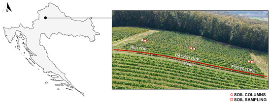
Figure 1.
SUPREHILL CZO location in Croatia with the aerial image of hilltop, backslope and footslope positions.
Disturbed soil samples (0–30 cm) were taken in triplicate at the hilltop, backslope, and footslope (Figure 1) within the machinery wheel track to determine physicochemical soil properties and were prepared according to the standardized sample preparation method for physical and chemical analyses (ISO 11464:2006). Soil particle size distribution was determined according to International Organization for Standardization—ISO 11277:2004. Soil texture at the surface depth (0–30 cm) of hillslope is classified as silt loam (USDA-NRCS, 2018). Based on the slope, the observatory is divided into two parts—17.5% (hilltop–backslope) and 25.4% (backslope–footslope). Long-term (1972–2022) average annual precipitation and temperature recorded at nearby Maksimir meteorological station were 856.5 mm and 11.2 °C, respectively. Organic carbon (Corg) content was determined according to ISO 14235:1998, and bulk density was determined using HYPROP-FIT [28]. Table 1 shows physical and chemical characteristics of soil at the investigated location with the standard deviation between replicates taken from the hilltop, backslope and footslope. Soil particle sizes are divided into coarse sand, 2.0–0.2 mm; fine sand, 0.2–0.063 mm; coarse silt, 0.063–0.02 mm; fine silt, 0.02–0.002; and clay, <0.002 mm.

Table 1.
Physicochemical soil properties with standard deviations of the investigated vineyard at a depth of 0–30 cm taken from the hilltop, backslope, and footslope in triplicate.
2.2. Soil Hydraulic Properties Estimation
Undisturbed soil cores (250 cm3; n = 9) were taken at the hilltop, backslope and footslope to determine soil hydraulic properties (SHP) at 0–30 cm depth. To ensure replicates at each position, three undisturbed soil cores were taken from the same position. Undisturbed soil cores were set in the plastic basin in the laboratory until full saturation. After the saturation, the soil cores were set on the sensor unit in the laboratory to estimate SHPs using the evaporation method [29] and the HYPROP automatized system [30]. Two tensiometers were placed at predefined positions inside the undisturbed soil sample at two depths (1.25 and 3.75 cm, respectively) to measure the soil water tension during the drying process [31]. The analysis is based on the Wind method [32] and uses the change in the hydraulic potential from tensiometer measurements in relation to water content changes to derive hydrological parameters. At the end of the evaporation method, i.e., when the second tensiometer reached the air entry value, the tensiometers were removed from the samples. For further measurements, subsamples were prepared. Two subsamples were taken from the top, middle and bottom part of the undisturbed soil core and placed in the sample cup for measurement. These subsamples were used to determine matric and osmotic potential, which completes the soil water characteristic curve (SWCC) and points at the dry end of the retention curve using the WP4C (dew-point soil water potential) device [33,34]. Soil hydraulic properties as well as water retention characteristic curves and hydraulic conductivity curves were determined using the HYPROP-FIT program [28].
SHPs were estimated using the van Genuchten–Mualem (VGM) single porosity model [35]:
where and denote residual and saturated volumetric water contents (L3 L−3), respectively; h is the pressure head (L); is the effective saturation (-); (L−1) and n (-) are shape parameters; and l (-) is a pore connectivity parameter and, in this study, was fixed to a value of 0.5, commonly used in most soil types [36].
The reliability of the soil hydraulic properties fitting was evaluated by root mean square error (RMSE), which indicates the mean distance between data point and the fitted function [37]. Coefficient of determination (R2) was used as a fitting parameter for soil hydraulic properties as well, and the two are calculated as follows:
where and are measured model predicted quantities, i.e., water content or hydraulic conductivities. The model error for water retention (RMSE_) was calculated separately from the model error for hydraulic conductivity (RMSE_K).
2.3. Water Flow Dynamics Estimation Using Undisturbed Soil Columns
Undisturbed soil columns, 25 cm in depth and 16 cm in diameter, were taken from the hilltop, backslope and footslope in triplicates (n = 9) from the inter-row area of a vineyard covered with grass. Triplicates were taken one above the other to ensure each soil column has the same environmental conditions. A non-reactive glue and quartz sand were applied to the column walls before the sample was taken to allow better fitting of the soil and to prevent the edge effect of water leaching alongside column walls. Undisturbed soil was excavated by pushing the columns into the soil [1,38]. Undisturbed soil columns experiment was conducted in controlled conditions in the laboratory where columns were saturated from the bottom and afterwards left to drain for 24 h before the leaching experiment to ensure the same conditions in each soil column, i.e., reach of the field capacity. An inert quartz material as well as a fine fiberglass mesh was placed at the bottom of each soil column to allow a small suction (−5 cm) and to prevent soil material disturbance.
EC-5 volumetric water content sensors (METER Group, Pullman, WA, USA) and mini tensiometers T5X (METER Group, Pullman, USA) were set in each soil column at 7 and 17 cm depth, respectively, with a reading resolution of 15 min. Potassium bromide (KBr) was applied with 150 mL in concentration 1 g L−1 at the top of the soil column. Each soil column was irrigated twice a day with 250 mL (5 mm h−1) of collected rainwater for 16 days using a hand sprayer to ensure uniform water application. Rainwater was collected in a barrel and analyzed before application to ensure proper conditions of an applied water, i.e., water that does not contain any element that could interfere with bromide concentration. Water samples (leachate) were collected twice a day and analyzed for Br− concentration using bromide ion-selective electrode (HI4102; Hanna Instruments, Woonsocket, RI, USA). Statistical data processing was carried out regarding the position on the slope from which the columns were taken using the SAS program [39]. One-way ANOVA and Tukey’s honest significant difference test (HSD test) at p < 0.05 were used to determine the significance of the difference between mean values. Subsequently, Brilliant Blue dye was applied on each soil column in the form of solute (10 g L−1) to determine the amount of the stained area, i.e., to identify and quantify preferential pathways. The dye tracer solution was divided into 100 mL dosages (to avoid buildup of the water layer at the top), and 800 mL in total was added on each soil column using a handheld sprayer. After leachate application, the columns were cut vertically in half. Slices were cut into 2.5 cm segments each, which resulted in six slices per column. Soil slices were photographed and analyzed using ImageJ software by creating binary images with stained and unstained area and calculating the stained amount. The procedure is described in detail in Filipović et al. (2020) [1].
3. Results and Discussion
3.1. Soil Hydraulic Properties Estimation
Soil hydraulic properties (Table 2) and soil water retention and hydraulic conductivity curves (Figure 2 and Figure 3) were estimated using HYPROP-FIT software. Similar values of the replicates used for the estimation of soil hydraulic properties indicated the reliability of the applied method. Porosity varied from 47% in the backslope and 51% for the hilltop to 54% at the footslope. Saturated volumetric water content (θs) values were in line with porosity and varied from 0.455 cm3 cm−3 in the backslope and 0.486 cm3 cm−3 at the hilltop to 0.496 cm3 cm−3 at the footslope. Consequently, the saturated hydraulic conductivity (Ks) was the highest at the footslope at 142.50 cm day−1, followed by 13.10 cm day−1 at the hilltop, and it was the lowest at the backslope with a value of 2.53 cm day−1. On the other hand, the bulk density (Table 1) was the highest in the backslope (1.4 g cm−3) and the lowest at the footslope (1.2 g cm−3).
Table 2.
Estimated soil hydraulic properties in the soil at different location on a hillslope obtained using HYPROP and WP4C device and determined using the HYPROP-FIT program.
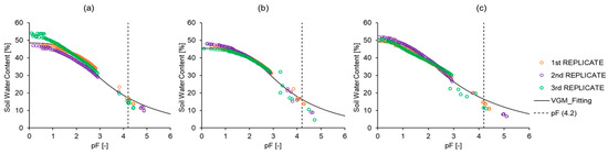
Figure 2.
Soil water retention curve determined for the (a) hilltop, (b) backslope and (c) footslope using HYPROP-FIT and fitted using the VGM model.
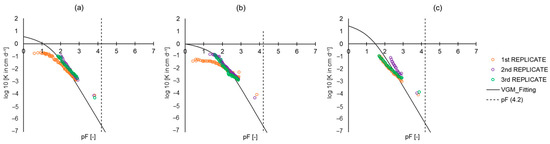
Figure 3.
Hydraulic conductivity curve determined for the (a) hilltop, (b) backslope and (c) footslope using HYPROP-FIT and fitted using the VGM model.
R2_θ was 0.9963 for the hilltop, 0.9926 for the backslope and 0.9920 for the footslope, and R2_K was 0.9993 for the hilltop and the backslope and 0.9992 for the footslope, indicating high model efficiency. According to RMSE_θ and RMSE_K, the van Genuchten–Mualem model was applicable for all measurements.
According to SWCC estimation and VGM fitting, the footslope has the highest saturated water content as a possible result of having the highest Corg (12.4 g kg−1) compared to other locations, which is in line with several other studies, e.g., [38,40]. According to these studies, Corg has the positive impact on the water retention capacity of soil. Furthermore, the differences in Ks throughout the hillslope could be a result of soil erosion, bulk density [41] and Corg (Table 1) [42] but are most likely due to the better pore connectivity. Standard deviation of the Ks showed wide variability, especially at the footslope, even though total porosity was not that variable. However, total porosity does not give information about the micro- and macropore ratio and pore connectivity [43]. The obtained results suggest that not only the ratio of micro-and macropores differs but also pore connectivity. Additionally, at the footslope, the slope is less pronounced resulting in greater vertical flow and the erosion of the fine particles towards the deeper horizons. Furthermore, through the years, eroded material from the whole hillslope was accumul ating in the footslope resulting in a deeper Apg horizon at this position [2,4], which could cause higher hydraulic conductivity.
3.2. Soil Column Experiments: Water Dynamics and Tracer Transport
3.2.1. Soil Water Measurements Using Sensor and Tensiometer
Figure 4 shows differences in soil water content during the drying and rewetting process, while Figure 5 shows tensiometer readings, i.e., changes in matric potential. Both the volumetric water content sensor (EC-5) and mini tensiometer (T5X) reacted shortly after irrigation with the drying process commencing thereafter. On average during the 16-day period, the tensiometer showed the highest values of the matric potential in the column taken from the backslope (3.4 hPa), followed by 0.6 hPa at the hilltop, and the lowest values were at the footslope (−1.5 hPa); i.e., the applied rainwater passed faster through the soil columns taken from the footslope compared to the ones from the backslope, which were the wettest and took more time to drain. Furthermore, the volumetric water content sensors also showed the highest average values in the soil columns taken from the backslope (0.46 m3 m−3) and showed the lowest at the footslope (0.39 m3 m−3). Initial water content was different even at the same position and was especially pronounced at the footslope, where these differences were the highest compared to the estimated θs. This, once again, suggests better pore connectivity at the footslope and the highest Ks, which resulted in more water drained from the soil column in 24 h. Further examination of the first replicate taken from the backslope revealed that a larger pore was present near the sensor head placement, possibly causing higher soil water content (even higher than saturated water content estimated using HYPROP-FIT) during the experiment as well as a different initial condition in this replicate compared to the second and third replicate, as seen in Figure 4b.
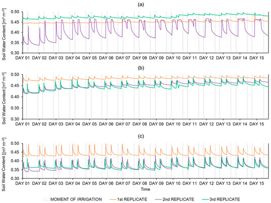
Figure 4.
Changes in soil water content in time between two irrigations (250 mL of rainwater) set at 7 cm depth inside undisturbed soil columns taken from the (a) hilltop, (b) backslope and (c) footslope.
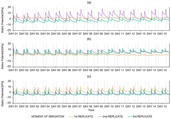
Figure 5.
Changes in matric potential in time between two irrigations (250 mL of rainwater) set at 17 cm depth inside undisturbed soil columns taken from the (a) hilltop, (b) backslope and (c) footslope.
Both the EC-5 sensor and T5X tensiometer showed that, on average, the column taken from the footslope is drier compared to the column taken from the backslope. The soil hydraulic properties showed the same results. As mentioned earlier, the highest θs was at the footslope, which is in line with other findings [44], which also had the highest Ks and porosity. Thus, the applied rainwater leached faster through the soil column taken from the footslope than from other locations, resulting in not only a more pronounced drying process but also the lowest soil water content values. In addition, the tensiometer showed drier soil in the column from the footslope due to the lower content of clay particles, causing higher permeability, which then results in lower soil water retention. This result is in line with other findings [42] claiming that the clay particles have a positive impact on water retention. On the contrary, the column taken from the backslope was the wettest due to an extremely low Ks, causing a greater time required for the water to pass through the soil column and resulting in the slowest drying and thus less pronounced drying process.
3.2.2. Water Flow Dynamics Estimation Using Bromide Tracer
Even though sensors and tensiometers showed differences in water content and matric potential, the statistical data in Table 3 show no significant difference between the mean volume values at the hilltop, backslope and the footslope. Similar uniform outflow was recorded in another study [45]. Further, the mean concentration values are not significantly different and vary from 22.49 mg L−1 at the backslope to 39.37 mg L−1 at the hilltop. However, the mean mass of bromide in the leached samples showed statistically significant differences for all three positions. The highest mean value of the mass of bromide was at the footslope (6.59 mg), while the lowest was at the hilltop (0.21 mg).
Table 3.
Impact of the soil column position on the hillslope on leached volume, bromide concentration and the mass of bromide. Letters a, b and c indicate significant differences between hillslope positions.
Figure 6 shows changes in leached bromide concentrations depending on percolated volume. It can be seen that at the hilltop and backslope most of the applied bromide was leached in the first few samples, while at the footslope, these changes were less pronounced and the bromide leaching per sample was more uniform. Furthermore, the concentration in the first sample in the columns from the hilltop and the backslope were much higher compared to ones from the footslope (Figure 6). This could be a result of heterogeneities in soil properties caused by soil erosion that was previously determined at this hillslope [4]. Soil erosion is common on the hillslope soils resulting in a looser layer at the footslope. As a consequence of soil tillage, the compacted less permeable layer is often present at the tillage depth. Accordingly, as a result of the soil erosion subsurface, the less permeable layer is at a shallower depth at the upper position compared to the footslope causing a more lateral preferential flow at the upper position in the field. As the results showed, hydraulic conductivity is the highest at the footslope due to better soil structure and pore connectivity resulting in larger vertical preferential flow and higher leached mass of bromide. Since the hilltop and backslope has lower hydraulic conductivity compared to the footslope, it is possible that the first few leachate samples (mostly the first two) were more concentrated due to the greater time necessary for passing through the soil column. Furthermore, that can cause most of the bromide to be leached in the beginning. Additionally, as mentioned earlier, the water content in these soil columns was higher compared to the water content in the soil columns taken from the footslope, causing a more steady flow; i.e., intermittent irrigation was less pronounced compared to the conditions in the column taken from the footslope. Due to the highest hydraulic conductivity at the footslope, the water flow was faster, resulting in the highest mean leached mass of bromide, which is in line with other studies, e.g., [45]. Similarly, to these results, they found that intermittent flow increased solute leaching compared to a steady flow.
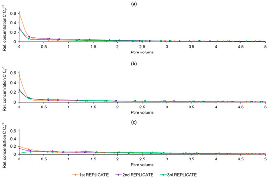
Figure 6.
Change in percolated bromide concentration depending on sample volume in soil columns (three replicates) taken from the (a) hilltop, (b) backslope and (c) footslope.
The differences in the mean values of the mass of bromide in the columns taken from the footslope are a result of physicochemical soil properties as well as soil hydraulic properties [46]. Since, at this position, the porosity and hydraulic conductivity are the highest, added rainwater passes the fastest. However, during the outflow collection, this is not found because the time between the samplings was relatively long. That caused a seemingly uniform volume of leachate. Similarly, although bromide concentration was slightly different at each position, there were no significant differences (Table 3). On the other hand, mean mass values showed statistically significant differences between positions, suggesting that slope position influences solute transport. This is consistent with the previous research conducted at the study site, which showed a different isotopic signature of soil water and different infiltration patterns [47]. According to these results, at the footslope, more solute could be transported to deeper depths. This could result in different precipitation distribution along the hillslope; i.e., at the footslope, more water can enter the soil in forms of direct precipitation, surface runoff and subsurface flow, causing more solute to attach to the soil particles and possibly leading to subsequent rapid solute transport. Furthermore, as mentioned earlier, the footslope has a deeper loose layer due to the accumulation of eroded soil [3,4], which results in greater hydraulic conductivity.
3.2.3. Identification and Quantification of Preferential Flow Using Brilliant Blue Dye Tracer
The amount of the dyed area in the undisturbed soil columns for the hilltop, backslope and footslope was obtained from the image processing using ImageJ (Table 4). Additionally, Figure 7, Figure 8, Figure 9, Figure 10, Figure 11, Figure 12, Figure 13, Figure 14 and Figure 15 show original photos of each column’s slice (left picture) and black and white pictures after processing them in ImageJ (right picture) for the hilltop (Figure 7, Figure 8 and Figure 9), the backslope (Figure 10, Figure 11 and Figure 12) and the footslope (Figure 13, Figure 14 and Figure 15). Depending on the slice, the dyed area in the soil columns taken from the hilltop ranged from 20.82 to 37.57%, at the backslope from 18.63 to 37.81%, and at the footslope from 15.69 to 69.48%. From these results, it can be clearly seen that even the soil columns taken from the same position have a relatively wide range of the stained area and that the water flow differs. Additionally, the preferential flow pattern occurs in each soil column. This can be seen in Figure 7, Figure 8, Figure 9, Figure 10, Figure 11, Figure 12, Figure 13, Figure 14 and Figure 15, in which even the first centimeters of the soils are not equally dyed. Furthermore, especially in Figure 8, Figure 9, Figure 11, Figure 12 and Figure 15, preferential flow can be seen deeper in the soil column. It is evident that dye tracer is bypassing some areas of the soil. Even though these results show differences in preferential flow from previously presented methods, all replicates showed similar results. Considering that the undisturbed soil columns were taken from the topsoil, it is expected that the results can differ due to the root channel and soil fauna activity present in that layer [11,48]. Additionally, most of the grass roots are present to a 15–20 cm depth, which can impact pore connectivity and preferential flow pathways [49]. The first and second replicates taken from the backslope show lower pore connectivity, which is in line with a lower estimated Ks (Table 2). On the other hand, at the footslope, the second and especially the third replicate show the highest amount of dyed area as a result of higher pore connectivity, which caused the highest Ks. Figure 7 shows the first replicate taken at the hilltop, where, in the middle (1a), a change in permeability can be seen (horizontal dyed area). Similar results showed the third replicate at the backslope (Figure 12). In the field, this change in permeability would result in lateral preferential flow. Further, Figure 9 shows a third replicate at the hilltop where the flora activity can be seen (especially 1a, 1b, 2a and 2b). Most of the dyed area followed the root pathway. Figure 11 shows the second replicate at the backslope, where fauna activity can be seen (from approximately 13 to 18 cm). Dye tracer also stained these holes, which are a result of soil fauna activity. The experimental error can be seen in Figure 9(3b) and Figure 14(3b), in which side flow occurred even though the non-reactive glue and inert quartz material were applied.
Table 4.
Dyed area amount for hilltop, backslope and footslope (three replicates) obtained after image processing using ImageJ.
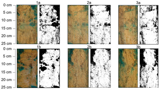
Figure 7.
Original photos of the dyed column’s slice (left) and after processing in ImageJ (right; black and white images) for the first replicate at the hilltop. Letter a represents the right half of the soil column, and b represents the left half of the column, while 1, 2 and 3 represent the number of the slice.
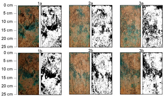
Figure 8.
Original photos of the dyed column’s slice (left) and after processing in ImageJ (right; black and white images) for the second replicate at the hilltop. Letter a represents the right half of the soil column, and b represents the left half of the column, while 1, 2 and 3 represent the number of the slice.
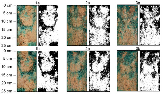
Figure 9.
Original photos of the dyed column’s slice (left) and after processing in ImageJ (right; black and white images) for the third replicate at the hilltop. Letter a represents the right half of the soil column, and b represents the left half of the column, while 1, 2 and 3 represent the number of the slice.
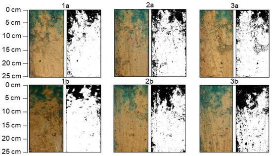
Figure 10.
Original photos of the dyed column’s slice (left) and after processing in ImageJ (right; black and white images) for the first replicate at the backslope. Letter a represents the right half of the soil column, and b represents the left half of the column, while 1, 2 and 3 represent the number of the slice.
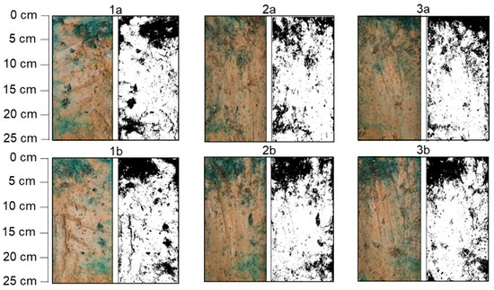
Figure 11.
Original photos of the dyed column’s slice (left) and after processing in ImageJ (right; black and white images) for the second replicate at the backslope. Letter a represents the right half of the soil column, and b represents the left half of the column, while 1, 2 and 3 represent the number of the slice.
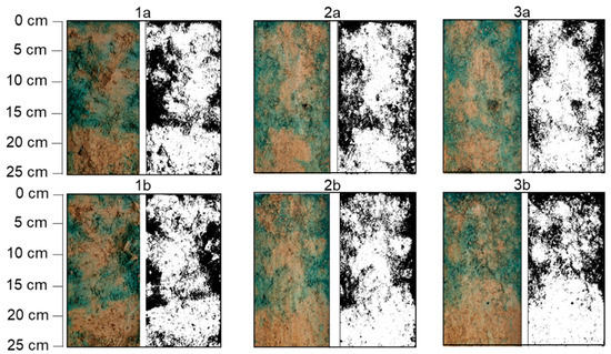
Figure 12.
Original photos of the dyed column’s slice (left) and after processing in ImageJ (right; black and white images) for the third replicate at the backslope. Letter a represents the right half of the soil column, and b represents the left half of the column, while 1, 2 and 3 represent the number of the slice.
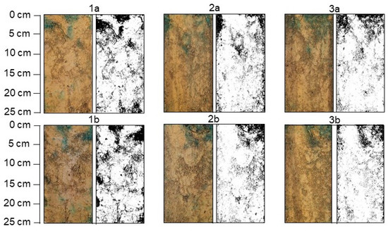
Figure 13.
Original photos of the dyed column’s slice (left) and after processing in ImageJ (right; black and white images) for the first replicate at the footslope. Letter a represents the right half of the soil column, and b represents the left half of the column, while 1, 2 and 3 represent the number of the slice.
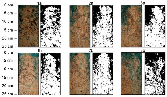
Figure 14.
Original photos of the dyed column’s slice (left) and after processing in ImageJ (right; black and white images) for the second replicate at the footslope. Letter a represents the right half of the soil column, and b represents the left half of the column, while 1, 2 and 3 represent the number of the slice.
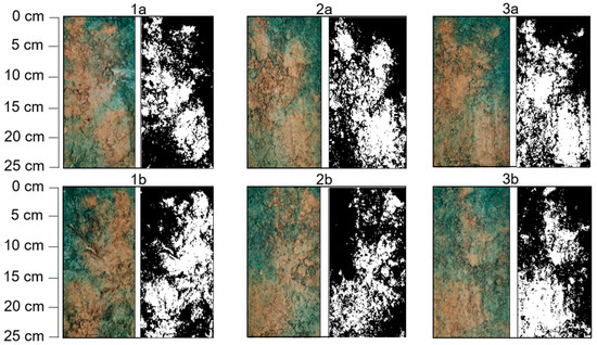
Figure 15.
Original photos of the dyed column’s slice (left) and after processing in ImageJ (right; black and white images) for the third replicate at the footslope. Letter a represents the right half of the soil column, and b represents the left half of the column, while 1, 2 and 3 represent the number of the slice.
4. Conclusions
This study revealed that the hillslope position has an impact on the soil’s physical, chemical and hydraulic properties due to soil erosion consequently causing different water flow velocities and solute transport in the soil. Differences were especially visible for the saturated hydraulic conductivity based on the different hillslope positions, which can be seen in the high standard deviations. On the other hand, total porosity was not so variable, suggesting that the differences in water flow were mostly impacted by pore connectivity, which consequently caused preferential flow. Tracer experiments showed a significant difference in the mass of the leached bromide with the highest values in the soil columns taken from the footslope, even though there were not significant differences in leached volumes. The results of sensor measurements were in line with the estimated SHPs, showing faster leaching of the irrigated rainwater in the footslope column. In general, tracer experiments showed the existence of preferential flow and soil heterogeneities even in the columns taken from the same position on the hillslope, which can be linked to plant roots and soil fauna activity. Altogether, the results showed the possible consequence of the deeper loose layer at the footslope as a consequence of soil erosion, which resulted in higher hydraulic conductivity and leached mean mass of the bromide due to better soil structure and pore connectivity. As a significant difference at relatively small area was determined, the research will be expanded in the field experiments to see the impact of the possible surface runoff and subsurface flow on a greater scale, which is common on the hillslope soils. The collected data also present valuable input for the calibration of water flow and solute transport models developed to simulate non-equilibrium transport processes in heterogenous soils.
Author Contributions
Conceptualization, J.D. and V.F.; methodology, J.D., V.K., L.F. and V.F.; software, J.D., V.K., L.F. and V.F.; validation, J.D., V.K., L.F. and V.F.; formal analysis, J.D. and V.F.; investigation, J.D., V.K., L.F., Z.K. and V.F.; data curation, J.D., V.K. and V.F.; writing—original draft preparation, J.D.; writing—review and editing, J.D., V.K., Z.K., V.P., H.H., T.B. and V.F.; visualization, J.D., V.K. and V.F.; supervision, V.F. All authors have read and agreed to the published version of the manuscript.
Funding
This research was funded by the Croatian Science Foundation, grant number UIP-2019-04-5409, under the following project name: “Subsurface preferential transport processes in agricultural hillslope soils—SUPREHILL”.
Institutional Review Board Statement
Not applicable.
Informed Consent Statement
Not applicable.
Data Availability Statement
Data are available on request from the corresponding author.
Conflicts of Interest
The authors declare no conflict of interest.
References
- Filipović, V.; Defterdarović, J.; Šimůnek, J.; Filipović, L.; Ondrašek, G.; Romić, D.; Bogunović, I.; Mustać, I.; Ćurić, J.; Kodešová, R. Estimation of Vineyard Soil Structure and Preferential Flow Using Dye Tracer, X-ray Tomography, and Numerical Simulations. Geoderma 2020, 380, 699. [Google Scholar] [CrossRef]
- Magdić, I.; Safner, T.; Rubinić, V.; Rutić, F.; Husnjak, S.; Filipović, V. Effect of Slope Position on Soil Properties and Soil Moisture Regime of Stagnosol in the Vineyard. J. Hydrol. Hydromech. 2022, 70, 62–73. [Google Scholar] [CrossRef]
- Herbrich, M.; Gerke, H.H.; Bens, O.; Sommer, M. Water Balance and Leaching of Dissolved Organic and Inorganic Carbon of Eroded Luvisols Using High Precision Weighing Lysimeters. Soil Tillage Res. 2017, 165, 144–160. [Google Scholar] [CrossRef]
- Filipović, V.; Defterdarović, J.; Krevh, V.; Filipović, L.; Ondrašek, G.; Kranjčec, F.; Magdić, I.; Rubinić, V.; Stipičević, S.; Mustać, I.; et al. Estimation of Stagnosol Hydraulic Properties and Water Flow Using Uni-and Bimodal Porosity Models in Erosion-Affected Hillslope Vineyard Soils. Agronomy 2022, 12, 33. [Google Scholar] [CrossRef]
- Filipović, V.; Coquet, Y.; Gerke, H.H. Representation of Plot-Scale Soil Heterogeneity in Dual-Domain Effective Flow and Transport Models with Mass Exchange. Vadose Zone J. 2019, 18, 174. [Google Scholar] [CrossRef]
- Cai, J.-S.; Yan, E.-C.; Yeh, T.-C.J.; Zha, Y.-Y. Effects of Heterogeneity Distribution on Hillslope Stability during Rainfalls. Water Sci. Eng. 2016, 9, 134–144. [Google Scholar] [CrossRef]
- Apollonio, C.; Petroselli, A.; Tauro, F.; Cecconi, M.; Biscarini, C.; Zarotti, C.; Grimaldi, S. Hillslope Erosion Mitigation: An Experimental Proof of a Nature-based Solution. Sustainability 2021, 13, 6058. [Google Scholar] [CrossRef]
- Nikodem, A.; Kodešová, R.; Fér, M.; Klement, A. Using Scaling Factors for Characterizing Spatial and Temporal Variability of Soil Hydraulic Properties of Topsoils in Areas Heavily Affected by Soil Erosion. J. Hydrol. 2021, 593, 125897. [Google Scholar] [CrossRef]
- Filipović, V.; Gerke, H.H.; Filipović, L.; Sommer, M. Quantifying Subsurface Lateral Flow along Sloping Horizon Boundaries in Soil Profiles of a Hummocky Ground Moraine. Vadose Zone J. 2018, 17, 106. [Google Scholar] [CrossRef]
- Guo, L.; Lin, H. Addressing Two Bottlenecks to Advance the Understanding of Preferential Flow in Soils, 1st ed.; Elsevier Inc.: Amsterdam, The Netherlands, 2018; Volume 147. [Google Scholar]
- Gerke, H.H. Preferential Flow Descriptions for Structured Soils. J. Plant Nutr. Soil Sci. 2006, 169, 382–400. [Google Scholar] [CrossRef]
- Nimmo, J.R. The Processes of Preferential Flow in the Unsaturated Zone. Soil Sci. Soc. Am. J. 2021, 85, 1–27. [Google Scholar] [CrossRef]
- Liu, Y.; Cui, Z.; Huang, Z.; López-Vicente, M.; Wu, G.L. Influence of Soil Moisture and Plant Roots on the Soil Infiltration Capacity at Different Stages in Arid Grasslands of China. Catena 2019, 182, 104147. [Google Scholar] [CrossRef]
- Wu, G.L.; Liu, Y.; Yang, Z.; Cui, Z.; Deng, L.; Chang, X.F.; Shi, Z.H. Root Channels to Indicate the Increase in Soil Matrix Water Infiltration Capacity of Arid Reclaimed Mine Soils. J. Hydrol. 2017, 546, 133–139. [Google Scholar] [CrossRef]
- Guo, L.; Liu, Y.; Wu, G.L.; Huang, Z.; Cui, Z.; Cheng, Z.; Zhang, R.Q.; Tian, F.P.; He, H. Preferential Water Flow: Influence of Alfalfa (Medicago sativa L.) Decayed Root Channels on Soil Water Infiltration. J. Hydrol. 2019, 578, 19. [Google Scholar] [CrossRef]
- Jarvis, N.J. A Review of Non-Equilibrium Water Flow and Solute Transport in Soil Macropores: Principles, Controlling Factors and Consequences for Water Quality. Eur. J. Soil Sci. 2007, 58, 523–546. [Google Scholar] [CrossRef]
- Liu, Y.; Li, S.; Shi, J.; Niu, Y.; Cui, Z.; Zhang, Z.; Wang, Y.; Ma, Y.; López-Vicente, M.; Wu, G.L. Effectiveness of Mixed Cultivated Grasslands to Reduce Sediment Concentration in Runoff on Hillslopes in the Qinghai-Tibetan Plateau. Geoderma 2022, 422, 115933. [Google Scholar] [CrossRef]
- Patil, M.D.; Das, B.S. Assessing the Effect of Puddling on Preferential Flow Processes through under Bund Area of Lowland Rice Field. Soil Tillage Res. 2013, 134, 61–71. [Google Scholar] [CrossRef]
- Dusek, J.; Dohnal, M.; Snehota, M.; Sobotkova, M.; Ray, C.; Vogel, T. Transport of Bromide and Pesticides through an Undisturbed Soil Column: A Modeling Study with Global Optimization Analysis. J. Contam. Hydrol. 2015, 175–176, 1–16. [Google Scholar] [CrossRef]
- Pietrzak, D.; Kania, J.; Kmiecik, E.; Wator, K. Identification of Transport Parameters of Chlorides in Different Soils on the Basis of Column Studies. Geologos 2019, 25, 225–229. [Google Scholar] [CrossRef]
- Beck-Broichsitter, S.; Gerriets, M.R.; Gerke, H.H.; Sobotkova, M.; Dusek, J.; Dohrmann, R.; Horn, R. Brilliant Blue Sorption Characteristics of Clay-Organic Aggregate Coatings from Bt Horizons. Soil Tillage Res. 2020, 201, 104635. [Google Scholar] [CrossRef]
- Kodešová, R.; Němeček, K.; Žigová, A.; Nikodem, A.; Fér, M. Using Dye Tracer for Visualizing Roots Impact on Soil Structure and Soil Porous System. Biologia 2015, 70, 1439–1443. [Google Scholar] [CrossRef]
- Flury, M.; Flühler, H. Brilliant Blue FCF as a Dye Tracer for Solute Transport Studies—A Toxicological Overview. J. Environ. Qual. 1994, 23, 1108–1112. [Google Scholar] [CrossRef] [PubMed]
- Clay, D.E.; Zheng, Z.; Liu, Z.; Clay, S.A.; Trooien, T.P. Bromide and Nitrate Movement through Undisturbed Soil Columns. J. Environ. Qual. 2004, 33, 338–342. [Google Scholar] [CrossRef]
- Kumar, A.; Ramola, A.; Kandwal, A.; Vidyarthi, A. Soil Moisture Sensor for Agricultural Applications Inspired from State of Art Study of Surfaces Scattering Models & Semi-Empirical Soil Moisture Models. J. Saudi Soc. Agric. Sci. 2021, 20, 559–572. [Google Scholar] [CrossRef]
- Yu, L.; Gao, W.; Shamshiri, R.R.; Tao, S.; Ren, Y.; Zhang, Y.; Su, G. Review of Research Progress on Soil Moisture Sensor Technology. Int. J. Agric. Biol. Eng. 2021, 14, 32–42. [Google Scholar] [CrossRef]
- Zhang, X.; Yang, C.; Wang, L. Research and Application of a New Soil Moisture Sensor. MATEC Web Conf. 2018, 175, 02010. [Google Scholar] [CrossRef]
- UMS. Meter Hyrop-Fit—Operation Manual; UMS: Munich, Germany, 2015. [Google Scholar]
- Schindler, U.G.; Müller, L. Soil Hydraulic Functions of International Soils Measured with the Extended Evaporation Method (EEM) and the HYPROP Device. Open Data J. Agric. Res. 2017, 3, 10–16. [Google Scholar] [CrossRef]
- Haghverdi, A.; Öztürk, H.S.; Durner, W. Measurement and Estimation of the Soil Water Retention Curve Using the Evaporation Method and the Pseudo Continuous Pedotransfer Function. J. Hydrol. 2018, 563, 251–259. [Google Scholar] [CrossRef]
- Campbell, G.; Campbell, C.; Cobos, D.; Crawford, L.B.; Rivera, L.; Chambers, C. Operation Manual for HYPROP; UMS: Munich, Germany, 2015; pp. 1–95. [Google Scholar]
- Wind, G.P. Capillary Conductivity Data Estimated by a Simple Method. Water Unsaturated Zone Proc. Wagening. Symp. 1969, 1, 181–191. [Google Scholar]
- Bin Shokrana, M.S.; Ghane, E. Measurement of Soil Water Characteristic Curve Using HYPROP2. MethodsX 2020, 7, 840. [Google Scholar] [CrossRef]
- Decagon Device Inc. WP4C Dew Point PotentiaMeter. Operator’s Manual; Decagon Device Inc.: Washington, DC, USA, 2013; ISBN 5093325600. [Google Scholar]
- Van Genuchten, M.T. A Closed-Form Equation for Predicting the Hydraulic Conductivity of Unsaturated Soils. Soil Sci. Soc. Am. J. 1980, 44, 892–898. [Google Scholar] [CrossRef]
- Mualem, Y. A New Model for Predicting the Hydraulic Conduc. Water Resour. Res. 1976, 12, 513–522. [Google Scholar] [CrossRef]
- Pertassek, T.; Peters, A.; Durner, W.; Data, H.; Software, E.; Durner, W. HYPROP Data Evaluation Software; User’s Manual; UMS: Munich, Germany, 2011; pp. 1–47. [Google Scholar]
- Kodešová, R.; Šimůnek, J.; Nikodem, A.; Jirků, V. Estimation of the Dual-Permeability Model Parameters Using Tension Disk Infiltrometer and Guelph Permeameter. Vadose Zone J. 2010, 9, 213–225. [Google Scholar] [CrossRef]
- SAS Institute Inc. SAS Enterprise Guide 8.3: Guía Del Usuario; SAS Institute: Cary, NC, USA, 2020; p. 564. [Google Scholar]
- Ankenbauer, K.J.; Loheide, S.P. The Effects of Soil Organic Matter on Soil Water Retention and Plant Water Use in a Meadow of the Sierra Nevada, CA. Hydrol. Process. 2017, 31, 891–901. [Google Scholar] [CrossRef]
- Kool, D.; Tong, B.; Tian, Z.; Heitman, J.L.; Sauer, T.J.; Horton, R. Soil Water Retention and Hydraulic Conductivity Dynamics Following Tillage. Soil Tillage Res. 2019, 193, 95–100. [Google Scholar] [CrossRef]
- Mashalaba, L.; Galleguillos, M.; Seguel, O.; Poblete-Olivares, J. Predicting Spatial Variability of Selected Soil Properties Using Digital Soil Mapping in a Rainfed Vineyard of Central Chile. Geoderma Reg. 2020, 22, e00289. [Google Scholar] [CrossRef]
- Defterdarović, J.; Filipović, L.; Kranjčec, F.; Ondrašek, G.; Kikić, D.; Novosel, A.; Mustać, I.; Krevh, V.; Magdić, I.; Rubinić, V.; et al. Determination of Soil Hydraulic Parameters and Evaluation of Water Dynamics and Nitrate Leaching in the Unsaturated Layered Zone: A Modeling Case Study in Central Croatia. Sustainability 2021, 13, 6688. [Google Scholar] [CrossRef]
- Liu, R.; Pan, Y.; Bao, H.; Liang, S.; Jiang, Y.; Tu, H.; Nong, J.; Huang, W. Variations in Soil Physico-Chemical Properties along Slope Position Gradient in Secondary Vegetation of the Hilly Region, Guilin, Southwest China. Sustainability 2020, 12, 1303. [Google Scholar] [CrossRef]
- Glæsner, N.; Diamantopoulos, E.; Magid, J.; Kjaergaard, C.; Gerke, H.H. Modeling Solute Mass Exchange between Pore Regions in Slurry-Injected Soil Columns during Intermittent Irrigation. Vadose Zone J. 2018, 17, 1–10. [Google Scholar] [CrossRef]
- Durner, W.; Flühler, H. Soil Hydraulic Properties. Encycl. Hydrol. Sci. 2005, 2005, 77. [Google Scholar] [CrossRef]
- Kovač, Z.; Krevh, V.; Filipović, L.; Defterdarović, J.; Buškulić, P.; Han, L.; Filipović, V. Utilizing Stable Water Isotopes (Δ2H and Δ18O) to Study Soil-Water Origin in a Sloped Vineyard: First Results. Rud. Geol. Naft. Zb. 2022, 37, 231. [Google Scholar] [CrossRef]
- Sander, T.; Gerke, H.H. Modelling Field-Data of Preferential Flow in Paddy Soil Induced by Earthworm Burrows. J. Contam. Hydrol. 2009, 104, 126–136. [Google Scholar] [CrossRef] [PubMed]
- Vereecken, H.; Weihermüller, L.; Assouline, S.; Šimůnek, J.; Verhoef, A.; Herbst, M.; Archer, N.; Mohanty, B.; Montzka, C.; Vanderborght, J.; et al. Infiltration from the Pedon to Global Grid Scales: An Overview and Outlook for Land Surface Modeling. Vadose Zone J. 2019, 18, 191. [Google Scholar] [CrossRef]


Disclaimer/Publisher’s Note: The statements, opinions and data contained in all publications are solely those of the individual author(s) and contributor(s) and not of MDPI and/or the editor(s). MDPI and/or the editor(s) disclaim responsibility for any injury to people or property resulting from any ideas, methods, instructions or products referred to in the content. |
© 2023 by the authors. Licensee MDPI, Basel, Switzerland. This article is an open access article distributed under the terms and conditions of the Creative Commons Attribution (CC BY) license (https://creativecommons.org/licenses/by/4.0/).