Abstract
The occurrence of catastrophic floods will increase the uncertainty of hydrological forecasting at downstream hydrological stations. In order to solve the problems of the unclear propagation law of catastrophic floods in the middle and lower reaches of the Yangtze River and the inadaptability of traditional forecasting methods, this paper uses the M-K trend test method to analyze the annual average flow and annual average water level of the Yichang and Hankou stations. For conventional floods and catastrophic floods, Random Forest (RF), Convolutional Neural Network (CNN), Long Short-Term Memory Network (LSTM), and CNN-LSTM neural networks are used to simulate the water level/flow of Hankou station. The simulation results are analyzed by Nash–Sutcliffe Efficiency Coefficient (NSE), Kling–Gupta efficiency coefficient (KGE), Root Mean Square Error (RMSE), and Symmetric Mean Absolute Percentage Error (SMAPE). The results show that the annual average flow and annual average water level of Yichang station show a downward trend and the annual average water level of Hankou station shows an upward trend. By comparing the four indicators of NSE, KGE, RMSE, and SMAPE, the CNN-LSTM coupling model was determined to be the best fitting model, with NSE and KGE greater than 0.995 and RMSE and SMAPE less than 0.200. The proposed coupling model can provide technical support for flood control optimization, scheduling, emergency rescue, and scheduling impact analysis of the Three Gorges Power Station.
1. Introduction
In recent years, frequent extreme weather events, uneven distribution of regional precipitation during the year, and flood disasters caused by extreme weather have caused serious losses to China’s social economy. In order to meet the needs of flood control and drought relief or emergency rescue in a concentrated period of time, the water conservancy and hydropower project increases or reduces the steep flow process formed by discharge, which is called catastrophic floods. As the most important water conservancy facility in China, the Three Gorges Reservoir will have a sudden discharge during the dispatching process, resulting in a sudden change in the water level and flow of the downstream river in a short time, which is easy to form a catastrophic flood. The occurrence of catastrophic floods will increase the uncertainty of hydrological forecasting at downstream hydrological stations, the result being that the water level and flow cannot be predicted timely and accurately. At the same time, there are many rivers and lakes in the middle reaches of the Yangtze River in China, and the water network is developed. The interaction between tributaries and lakes is complex. It is particularly critical to use more advanced methods to construct relevant hydrological models in the context of global climate change.
In order to deeply understand the influence of catastrophic floods and conventional floods on the prediction of downstream water level and flow, many scholars have conducted extensive research on this hot issue based on different methods and models. Li Xiaoyang [1] coupled the Variable Infiltration Capacity (VIC) runoff model with the improved distributed confluence model to realize the hourly flood forecasting based on the VIC model and verified it in the Biliu River Basin. Zhang Hongbo [2] quantified the variation characteristics of the runoff series of the three rivers in Jingnan, introduced the STARS method and the ICSS method to identify the mean and variance changes of the runoff series, and determined the variation position and variation level. At the same time, by combining the major human activities that occurred during the same period, the driving causes of runoff variation in the three rivers in Jingnan were explored from the perspective of physical mechanisms. Wang Zhiyong [3] extended the branch water level prediction and correction method for river network calculation to the one-dimensional-two-dimensional model coupling problem, proposed the coupled boundary water level prediction and correction method, and established a numerical model suitable for the overall hydrodynamic simulation of a river–lake system.
The neural network is the core of the deep learning algorithm. With the rapid development of computer hardware and the continuous improvement of data sets, the neural network artificial intelligence algorithm has been widely used in the field of hydrological forecasting. Zhang et al. (2021) [4] improved the prediction method of reservoir downstream water level by using the convolutional neural network (CNN) and the long short-term memory network (LSTM), and improved the calculation accuracy of reservoir power generation output. Guan Jie [5] started from the practical application scenario of water level early warning in the middle and lower reaches of the Chishui River. On the basis of fully studying the relevant theoretical techniques of water level prediction based on machine learning, three machine learning algorithms based on multiple linear regression (MLR), extreme random tree (Extra-Tress), and artificial neural network (ANN) were constructed. Based on the two-dimensional convolutional neural network, Ji Zhansheng et al. [6] constructed the water level prediction method of the Pingyao hydrological station in Dongtiaoxi, selected the rising water level, downstream water level, upstream reservoir discharge, and interval precipitation to construct the feature set, and extracted the effective features of the input feature set. Although the above research based on neural networks is of great significance in the study of the complex hydrological relationship between the mainstream, tributaries, and lakes, unfortunately, the artificial neural feedforward network (BP), random forest (RF), and support vector machine (SVM) methods [7,8,9,10,11,12,13,14] are mostly used in the network between hydrological variables, which have high training complexity and are not easy to extract features from. In contrast, CNN can extract and reduce the dimension of important features through the convolution layer and the pooling layer. Combined with other neural networks or methods, CNN is used in the field of flood forecasting [15,16,17,18,19]. The long short-term memory network, LSTM, has the characteristics of maintaining the relationship between data in the sequence and has significant advantages in processing data with temporal relationships. At the same time, LSTM and its combinations are widely used in water level and flow forecasting [20,21,22,23,24].
Therefore, the main purpose of this study is to take the Yichang–Hankou section of the Yangtze River as the research area. In view of the unclear propagation law of the current catastrophic flood in the middle and lower reaches of the Yangtze River and the inadaptability of traditional forecasting methods, the M-K trend analysis method is used to analyze the average annual flow and average annual water level of Yichang station and Hankou station. On this basis, CNN and LSTM are introduced to construct the water level/flow prediction model, and the advantages of CNN and LSTM are integrated. The RF model, CNN, LSTM, and CNN-LSTM are used to predict the flow/water level of conventional floods and catastrophic floods. Finally, the optimal model is selected by combining NSE, KGE, RMSE, and SMAPE model evaluation indexes. The biggest innovation of this study is to define the catastrophic floods and put forward the optimal prediction model of water level/flow response of Hankou station based on the flow of Yichang station and the real-time fast and accurate estimation method. It provides technical support for flood control optimization, dispatching, emergency rescue, and dispatching impact analysis of the Three Gorges Power Station.
2. Materials and Methods
2.1. Study Area
This study takes the Yichang–Hankou section as the research area. The region is located in the middle reaches of the Yangtze River, 645 km long. The average annual temperature in this area is about −3–20 °C. The maximum temperature in some areas in summer can reach 40 °C. In winter, the temperature may drop to about 0 °C in some areas. Spring and autumn are transitional seasons, and the temperature is mild. The average annual precipitation is about 670–2300 mm. Summer is rainy and concentrated, with an average monthly rainfall of about 300 –500 mm. May to September is a flood-prone period. In winter, the precipitation is relatively low, and the monthly average rainfall is about 50–100 mm. The precipitation in spring and autumn is moderate, and the monthly average precipitation is between 100 and 200 mm. In the section, there are the Qingjiang River, the Juzhang River, the Dongting Lake, and the Hanjiang River. At the same time, we selected six hydrological stations as the key research objects, including Yichang (YC), Zhicheng (ZC), Shashi (SS), Jianli (JL), Chenglingji (CLJ), and Hankou (HK). The daily flow, water level, rainfall, evaporation, and temperature of the previous five stations were used as model input data to simulate the flow and water level of HK. The Yichang–Hankou section of the Yangtze River and hydrological stations are shown in Figure 1.
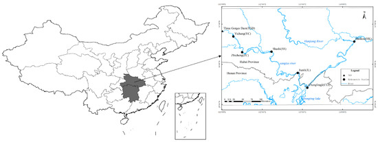
Figure 1.
Study Area.
2.2. Data Sources
The meteorological data of daily-scale water level, rainfall, evaporation, and temperature at six hydrological stations from 2008 to 2020 were obtained from the Yangtze River Water Resources Commission and Hubei Provincial Meteorological Bureau (http://www.cjw.gov.cn/, accessed on 14 May 2022). The reliability of the data is guaranteed by the reorganization of the relevant units. Based on the quantitative analysis of the outflow of the Three Gorges Reservoir from 2008 to 2020, this study determined that, in 2010, 2012, and 2017, due to the operation of the Three Gorges Reservoir, the middle and lower reaches of the river produced catastrophic floods. The flow chart is shown in Figure 2.
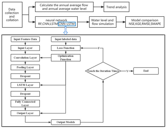
Figure 2.
Flow chart.
2.3. Trend Analysis
In this study, the Mann-Kendall trend test (M-K) [25] was used to analyze the hydrological trend. The advantage of this method is that it does not require the sequence to be detected to follow a certain distribution, the calculation is simple, and it is not disturbed by a few outliers. In the M-K test, let the null hypothesis be H0: the time series used is n independent samples, and each sample obeys the same distribution. The alternative hypothesis H1 is a two-sided test: for any k, j < n, and k ≠ j, the distribution of xk and xj is different. For any sequence Xt (t = 1, 2,…, n), n is the length of the sequence to be tested, and the statistic S can be defined:
where Xj and Xk are the time series corresponding year data, n is the length of the time series, and sgn (Xj − Xk) is a sign function.
2.4. Random Forest Model
The RF model is a combined classifier algorithm using Classification and Regression Tree (CART) as a meta-classifier. It consists of multiple decision trees. Each decision tree gives an independent classification result for the input. Finally, the final output is determined by a majority vote based on the classification results of all decision trees [26]. In the process of operation, RF mainly generates different training sets through a bootstrap self-sampling method to construct each meta-classifier. When the subset is generated by the sampling method, nearly 37% of the Out-of-Bag (OOB) data in the original sample will not appear in the new subset. These data are used to estimate the generalization error of RF to characterize the stability and accuracy of the model [27].
2.5. Convolutional Neural Network
CNN is a deep feed-forward neural network with local connection and weight sharing. It is generally a feed-forward neural network composed of a convolutional layer, a convergence layer, and a fully connected layer. By moving the receptive field to scan the whole, the feature of weight sharing greatly reduces the number of weight coefficients, reduces the complexity of the model, and makes it closer to the biological neural network [28]. The convolution layer in CNN is calculated by the convolution algorithm. The convolution formula is:
where a = (f − 1)/2, b = (h − 1)/2, f and h are odd integers, and i is the matrix to be convoluted.
2.6. Long Short-Term Memory Network
The LSTM is a variant of a recurrent neural network, which can effectively solve the problem of gradient explosion or disappearance of simple recurrent neural networks. The LSTM network introduces a new internal state ct dedicated to linear cyclic information transmission, while it (nonlinearly) outputs information to the external state ht of the hidden layer. The internal state ct is calculated by the following formula:
where is the vector element product, ct−1 is the memory unit of the previous moment, and is the candidate state obtained by the nonlinear function:
At each time t, the internal state ct of the LSTM network records the historical information up to the current time.
The LSTM network introduces a gating mechanism to control the path of information transmission. The gating mechanism includes the input gate it, forgetting gate ft, and output gate ot, which are:
- (1)
- The forgetting gate “ft” controls how much information needs to be forgotten in the internal state of the previous moment.
- (2)
- The input gate “it” controls the candidate state of the current moment, and how much information needs to be saved.
- (3)
- The output gate “ot” controls how much information the current internal state needs to be output to the external state.
When ft = 0, it = 1. The memory unit clears the historical information and writes the candidate state vector . However, the memory unit ct is still related to the historical information of the previous moment. When ft = 1, it = 0. The memory unit will copy the content of the previous moment and not write new information.
The calculation method is:
where is the logistic function, its output interval is (0, 1), xt is the input of the current time, and ht − 1 is the external state of the previous time. Through the LSTM loop unit, the entire network can establish long-distance temporal dependencies.
2.7. CNN-LSTM
Due to the time-varying water level and flow in flood forecasting, there are great errors in convolutional neural network (CNN) simulation. In this paper, the long short-term memory network (LSTM), which can maintain the relationship between the data in the sequence, is coupled with the convolutional neural network (CNN). The input data enter the LSTM network after the first dropout in the convolutional network and enter the fully connected layer after a dropout. The CNN-LSTM model combines the characteristics of the two networks. First, the data are input into the CNN, and the important features are extracted and reduced by the convolution layer and the pooling layer. Then, the full connection layer is input into the LSTM network unit and the model is obtained by multiple iterative training.
2.8. Model Goodness Evaluation
This study uses NSE, KGE for efficiency evaluation, RMSE, and SMAPE for error evaluation. When NSE and KGE are close to 1, the model fitting efficiency is the highest. The smaller the RMSE and SMAPE are, the smaller the model fitting error is.
3. Results
3.1. Trend Changes of Annual Average Flow and Annual Average Water Level
The M-K trend analysis method was used to study the trend changes of annual average flow and annual average water level of Yichang station and Hankou station from 1952 to 2020. See Figure 3 for the M-K trend analysis of the annual average flow of Yichang station. There are multiple intersections between the UF and UB curves in the confidence interval, which is the time when the annual average flow of Yichang station changes abruptly, such as 1989 and 1982. The UF curve is within the confidence interval, so the change of annual average flow is not significant and, since 1971, the annual average flow of Yichang station has generally shown a decreasing trend. The M-K trend analysis of the annual average flow of Hankou station shows that the UF and UB curves have multiple intersections in the confidence interval. From 1955 to 1965, the annual average flow of Hankou station showed a downward trend, and the downward trend was significant near 1960. From 1965 to 2003, the annual average flow trend tended to be stable. From 2003 to 2008, during the construction of the Three Gorges Reservoir, the annual average flow of Hankou station showed an increasing trend.
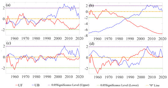
Figure 3.
Trend changes of annual average flow and annual average water level. Annual average flow trend analysis of Yichang station (a), annual average water level trend analysis of Yichang station (b), annual average flow trend analysis of Hankou station (c), and annual average water level trend of Hankou station (d).
The M-K trend analysis of the annual average water level of Yichang station shows that the intersection of the UF and UB curves is outside the confidence interval, indicating that the annual average water level of the station has a significant trend at the 95% significance level; that is, the trend is statistically significant. It can also be explained that the intersection of the UF curve and the UB curve outside the confidence interval means that there is evidence of real potential trends in the data, not just random variability. Since 1967, the annual average water level has shown a downward trend, and the downward trend was significant after 1984. The M-K trend analysis of the annual average water level of Hankou station is carried out. The UF and UB curves have multiple intersections in the confidence interval, located near 1976, 1979, 2003, 2004, and 2018. According to the UF curve, the average annual water level of Hankou station showed a downward trend from 1955 to 1990, and an increasing trend from 1990 to 2020. In general, the annual average water level change trend of Hankou station is not significant; there is only a significant downward trend near 1960.
3.2. Comparison of Simulation Results of Four Neural Network Models
The RF, CNN, LSTM, and CNN-LSTM coupled network models were used to train with data from 2008 to 2015 and validate with data from 2016 to 2020. The simulation results of the flow process and water level process in the flood period of Hankou station are shown in Figure 4 and Figure 5. In the single model, the prediction efficiency of the CNN model is low, the error is large, and the error distribution is scattered, which is not suitable for the prediction of flow and water level. The RF model can well reflect the flow change trend, and the predicted value can better fit the real value, but, in the prediction process, there will be a point where the predicted value and the real value differ greatly and the stability is poor. In the water level prediction, the RF model is more unstable and the simulation of the trend is not good. The LSTM network has both stability and accuracy. The comprehensive fitting effect of water level and flow is the best in a single model, which is more suitable for the prediction of water level and flow.
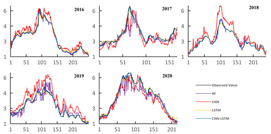
Figure 4.
Flow process simulation (abscissa is time (d), and the ordinate is flow (104 m3/s)).
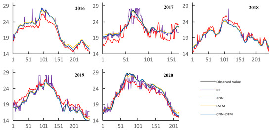
Figure 5.
Water level process simulation (abscissa is time (d), and the ordinate is water level (m)).
The coupled model, CNN-LSTM, is significantly better than the single model in the simulation of water level and flow. The advantages of CNN in dealing with multi-feature attributes and LSTM in dealing with time series make the simulation efficiency the highest and the stability the best. It is suitable for the prediction of water level flow.
3.3. Evaluation of Simulation Results
The observed value is the abscissa and the simulated value is the ordinate drawn in the coordinate system. The simulation results of the four models are evaluated according to the distribution trend of the points, as shown in Figure 6 and Figure 7.
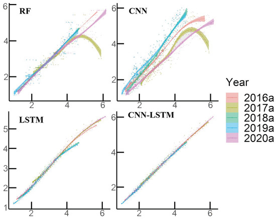
Figure 6.
Flow observation and simulation value distribution diagram (the abscissa is the observed value, the ordinate is simulated).
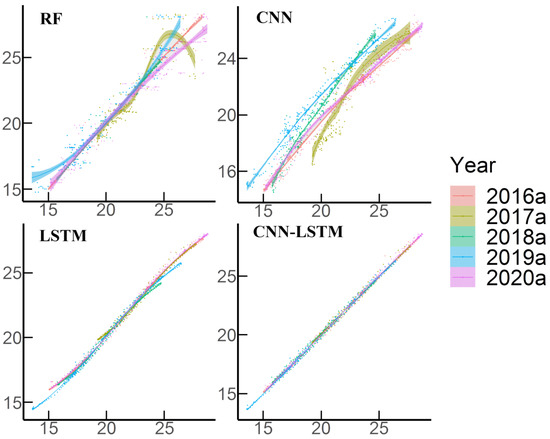
Figure 7.
Water level observation and simulation value distribution diagram (the abscissa is the observed value, the ordinate is the simulated).
In the conventional flood years (2016, 2018, 2019, 2020), in the single model flow simulation, the data points of the observed value and the simulated value of the CNN model are the most dispersed, indicating that the model fluctuates greatly in the process of simulating the flow. The fitting effect of the RF model in the low flow area is slightly better than that of the LSTM model, and the simulation error of the RF model in the high flow area increases slightly. The fitting degree of the full flow range of the LSTM model is similar, the simulation results in the low flow area are larger, and the simulation results in the high flow area are smaller. The coupling model is better than the single model in the whole flow section. In the simulation of the single model water level, the effect of the CNN model on different years is indeed different, and the stability of the model is not good. The RF model has obvious errors in both the high water level area and low water level area, and the error of the LSTM model in the high water level area is greater than that in the low water level area. The coupled model performs better than the single model in each water level section.
In the year of catastrophic floods (2017), in a single model, the CNN and RF models have obvious deviations in the high flow area and high water level area, among which the CNN model has a poor simulation effect on the low water level. The simulation effect of the LSTM model did not change much compared with the conventional flood. The simulation effect of the coupled model is still better than that of the single model.
Evaluation indexes of each model in each year are shown in Table 1. In terms of flow simulation in conventional flood years, the average NSE of the RF, CNN, LSTM, and CNN-LSTM coupled models were 0.947, 0.700, 0.986, and 0.995, respectively. The mean KGE was 0.955, 0.751, 0.929, and 0.984, respectively. The average RMSE was 0.238, 0.546, 0.134, and 0.074, respectively. The average SMAPE was 0.050, 0.150, 0.041, and 0.021, respectively. It shows that, in a single model, CNN has the worst simulation effect, and RF is close to the LSTM model. The indexes of the coupled model are better than those of the single model. In terms of water level simulation, the average NSE of the RF, CNN, LSTM, and CNN-LSTM coupled models are 0.946, 0.872, 0.991 and 0.997, respectively. The average KGE were 0.956, 0.845, 0.949, and 0.996, respectively. The average RMSE was 0.775, 1.212, 0.321, and 0.185, respectively. The average SMAPE was 0.021, 0.047, 0.013, and 0.007, respectively. It shows that, in a single model, CNN has the worst simulation effect, and RF is close to the LSTM model. The indexes of the coupled model are better than those of the single model.

Table 1.
Evaluation indexes of each model in each year.
In 2017, the catastrophic flood was caused by the operation of the Three Gorges Reservoir. In terms of traffic simulation, LSTM has the best simulation effect in the single neural network traffic model. The NSE and KGE of LSTM are 56.17% and 34.93% higher than those of the RF model, and 48.44% and 9.77% higher than those of the CNN model, respectively. The RMSE and SMAPE are 73.12% and 72.96% lower than the CNN model, respectively, and LSTM is 74.31% and 57.57% lower than the RF model, respectively. The simulation effect of the CNN-LSTM coupling model is similar to that of LSTM. The NSE and KGE of the coupling model are 1.17% and 5.93% higher than those of the LSTM model, and the SMAPE and RMSE are lower than 33.72% and 26.73%, respectively. In terms of water level simulation, LSTM has the best simulation effect in the single neural network water level prediction model. The NSE and KGE of LSTM are 42.47% and 15.98% higher than those of the RF model, and 133.20% and 26.88% higher than those of the CNN model, respectively. The RMSE and SMAPE are 81.53% and 83.97% lower than the CNN model, respectively, and LSTM is 74.83% and 68.84% lower than the RF model, respectively. The simulation effect of the CNN-LSTM coupled model is similar to that of LSTM. The NSE and KGE of the coupled model are 1.18% and 6.25% higher than those of the LSTM model, respectively, and the SMAPE and RMSE are lower than 40.78% and 35.83%, respectively.
In summary, CNN is not suitable for the simulation of water level and flow. The LSTM model and the RF model have similar effects on simulating flow. The LSTM model is better than the RF model when simulating water level, and the CNN-LSTM coupling model is better than the single model.
4. Conclusions
4.1. Trend
The trend analysis of the annual average flow and annual average water level of Yichang station and Hankou station shows that the annual average flow and annual average water level of Yichang station show a downward trend, the annual average flow of Hankou station has no obvious change, and the annual average water level shows an upward trend.
4.2. Model
The four neural networks of RF, CNN, LSTM, and CNN-LSTM were used to simulate the water level and flow of Hankou station by combining the hydrological and meteorological data of Yichang, Zhicheng, Shashi, Jianli, and Chenglingji. For conventional floods, in a single model, the CNN model has low prediction efficiency, large errors, and a more dispersed error distribution, which is not suitable for flow and water level prediction. The RF model can well reflect the flow change trend, and the predicted value can better fit the real value. However, in the prediction process, there will be a point where the predicted value and the real value differ greatly, and the stability is poor. In the water level prediction, the RF model is more unstable, and the simulation of the trend is not good. The LSTM network has both stability and accuracy. The comprehensive fitting effect of water level and flow is the best in a single model, which is more suitable for the prediction of water level and flow. The coupling model, CNN-LSTM, is indeed due to the single model in the simulation of water level and flow. The advantages of CNN in dealing with multi-feature attributes and LSTM in dealing with time series make the simulation efficiency the highest and the stability the best. It is suitable for the prediction of water level flow. For catastrophic floods, neither the RF nor CNN models can effectively simulate water level and flow, and the simulation results of LSTM and the coupling models are still excellent. In order to better quantify the degree of fitting, this paper uses NSE, KGE, RMSE, and SMAPE to analyze the simulation results. The average values of NSE and KGE in the coupling model are between 0.9830 and 0.9970, and RMSE and SMAPE are between 0.0050 and 0.2000; indeed, better than a single model.
5. Discussion
Since the Three Gorges Reservoir operated at the normal water level in 2008, there have been fewer years of catastrophic floods. Due to the lack of neural network training samples, the catastrophic floods have only been simulated for 2017. Although excellent prediction results have been achieved, the prediction efficiency lacks universality. The next step is to increase the catastrophic flood samples and further explore the adaptability and promotion value of the model. The influence of lakes along the river on its water level and flow and accurate simulation are also topics that need further study [29].
Author Contributions
Several authors contributed to create this research article. Detailed contributions were as follows: Conceptualization, Y.X.; Methodology, Y.X. and Y.C.; Software, Y.S. and Y.D.; Investigation, Y.X.; Formal analysis, Z.G.; Resources, Y.X.; Writing—original draft preparation, Z.G.; Writing—review and editing, C.H. and Y.C. All authors have read and agreed to the published version of the manuscript.
Funding
This research received funding from the Hubei Key Laboratory of Intelligent Yangtze and Hydroelectric Science, China Yangtze Power Co., Ltd. open research fund, Fund number: ZH2102000111.
Data Availability Statement
Not applicable.
Acknowledgments
We thank the Hubei Key Laboratory of Intelligent Yangtze and Hydroelectric Science, China Yangtze Power Co., Ltd. and Yangtze University for financial support for this study.
Conflicts of Interest
The authors declare no conflict of interest.
References
- Li, X.; Ye, L.; Wu, J.; Wang, J.; Zeng, F.; Zhou, H. Study on improvement of VIC model and its application in flood forecasting of river basins. Water Resour. Hydropower Eng. 2022, 53, 18–26. [Google Scholar]
- Zhang, H.; Cao, W.; Zhang, S.; Zhang, Y. Quantitative evaluation of Human-introduced runoff change of three streams in the Southern Jingjiang River of Dongting Lake area, China. J. Earth Sci. Environ. 2018, 40, 91–100. [Google Scholar]
- Wang, Z.; Chen, Y.; Zhu, D.; Liu, Z. 1D-2D coupled hydrodynamic simulation model of river-lake system. Adv. Water Sci. 2011, 22, 516–522. [Google Scholar]
- Zhang, Z.; Qin, H.; Yao, L.; Liu, Y.; Jiang, Z.; Feng, Z.; Ouyang, S.; Pei, S.; Zhou, J. Downstream Water Level Prediction of Reservoir based on Convolutional Neural Network and Long Short-Term Memory Network. J. Water Resour. Plan. Manag. 2021, 147, 04021060. [Google Scholar] [CrossRef]
- Guan, J. Research on Early Warning of Streamflow in the Middle and Lower Reaches of Chishui River Based on Machine Learning. Univ. Electron. Sci. Technol. China 2018. [Google Scholar]
- Ji, Z.; Zhang, G.; Zhang, Z. Water Level Forecast of Pingyao Hydrological Station in Dongtiaoxi Based on Convolutional Neural Network. Water Resour. Power 2021, 39, 46–49. [Google Scholar]
- Hu, Y.; Chen, T.; Luo, X.; Tang, C.; Liang, Z. Medium to Long Term Runoff Forecast for the Huai River Basin Based on Machine Learning Algorithm. Earth Sci. Front. 2022, 29, 284–291. [Google Scholar]
- Ji, Z.; Zhang, G.; Huang, W. Water Level Forecast Method of Plain River Network Based on Online SVM. J. Anhui Agric. Sci. 2021, 49, 191–195. [Google Scholar]
- Li, L.; Wang, Y.; Hu, Q.; Liu, D.; Zhang, A.; Ba, Y. Long-Term Inflow Forecast of Reservoir Based on Random Forest and Support Vector Machine. Hydro-Sci. Eng. 2020, 4, 33–40. [Google Scholar]
- Choi, C.; Kim, J.; Han, H.; Han, D.; Kim, H.S. Development of Water Level Prediction Models Using Machine Learning in Wetlands: A Case Study of Upo Wetland in South Korea. Water 2020, 12, 93. [Google Scholar] [CrossRef]
- Guyennon, N.; Salerno, F.; Rossi, D.; Rainaldi, M.; Calizza, E.; Romano, E. Climate change and water abstraction impacts on the long-term variability of water levels in Lake Bracciano (Central Italy): A Random Forest approach. J. Hydrol.-Reg. Stud. 2021, 37, 100880. [Google Scholar] [CrossRef]
- Mohammadi, B.; Guan, Y.Q.; Aghelpour, P.; Emamgholizadeh, S.; Zola, R.P.; Zhang, D.R. Simulation of Titicaca Lake Water Level Fluctuations Using Hybrid Machine Learning Technique Integrated with Grey Wolf Optimizer Algorithm. Water 2020, 12, 3015. [Google Scholar] [CrossRef]
- Nhu, V.H.; Shahabi, H.; Nguyen, H. Daily Water Level Prediction of Zrebar Lake (Iran): A Comparison between M5P, Random Forest, Random Tree and Reduced Error Pruning Trees Algorithms. ISPRS Int. J. Geo-Inf.-Ation 2020, 9, 479. [Google Scholar] [CrossRef]
- Chen, K.Y.; Chen, H.X.; Zhou, C.L.; Huang, Y.C.; Qi, X.Y.; Shen, R.Q.; Liu, F.R.; Zuo, M.; Zou, X.Y.; Wang, J.F.; et al. Comparative analysis of surface water quality prediction performance and identification of key water parameters using different machine learning models based on big data. Water Res. 2020, 171, 115454. [Google Scholar] [CrossRef] [PubMed]
- Kimura, N.; Yoshinaga, I.; Sekijima, K.; Azechi, I.; Baba, D. Convolutional Neural Network Coupled with a Transfer-Learning Approach for Time-Series Flood Predictions. Water 2020, 12, 96. [Google Scholar] [CrossRef]
- Wang, Y.; Fang, Z.C.; Hong, H.Y.; Peng, L. Flood susceptibility mapping using convolutional neural network frameworks. J. Hydrol. 2020, 582, 124482. [Google Scholar] [CrossRef]
- Panahi, M.; Jaafari, A.; Shirzadi, A.; Shahabi, H.; Rahmati, O.; Omidvar, E.; Lee, S.; Bui, D.T. Deep learning neural networks for spatially explicit prediction of flash flood probability. Geosci. Front. 2021, 12, 101076. [Google Scholar] [CrossRef]
- Li, P.F.; Zhang, J.; Krebs, P. Prediction of Flow Based on a CNN-LSTM Combined Deep Learning Approach. Water 2022, 14, 993. [Google Scholar] [CrossRef]
- Khosravi, K.; Panahi, M.; Golkarian, A.; Keesstra, S.D.; Saco, P.M.; Bui, D.T.; Lee, S. Convolutional neural network approach for spatial prediction of flood hazard at national scale of Iran. J. Hydrol. 2020, 591, 125552. [Google Scholar] [CrossRef]
- Fang, Z.C.; Wang, Y.; Peng, L.; Hong, H.Y. Predicting flood susceptibility using LSTM neural networks. J. Hydrol. 2021, 694, 125734. [Google Scholar] [CrossRef]
- Liu, M.Y.; Huang, Y.C.; Li, Z.J.; Tong, B.X.; Liu, Z.T.; Sun, M.K.; Jiang, F.Q.; Zhang, H.C. The Applicability of LSTM-KNN Model for Real-Time Flood Forecasting in Different Climate Zones in China. Water 2020, 12, 440. [Google Scholar] [CrossRef]
- Yang, M.Z.; Zhong, P.A.; Li, J.Y.; Liu, W.F.; Li, Y.H.; Yan, K.; Yuan, Y.Y.; Gao, Y.H. Research on intelligent prediction and zonation of basin-scale flood risk based on LSTM method. Environ. Monit. Assess. 2020, 192, 387. [Google Scholar] [CrossRef] [PubMed]
- Atashi, V.; Gorji, H.T.; Shahabi, S.M.; Kardan, R.; Lim, Y.H. Water Level Forecasting Using Deep Learning Time-Series Analysis: A Case Study of Red River of the North. Water 2022, 14, 1971. [Google Scholar] [CrossRef]
- Li, W.; Kiaghadi, A.; Dawson, C. Exploring the best sequence LSTM modeling architecture for flood prediction. Neural Comput. Appl. 2021, 33, 5571–5580. [Google Scholar] [CrossRef]
- Zhang, H.; Li, Z.; Xi, Q.; Yu, Y. Modified over-whitening process and its application in Mann-Kendall trend tests. J. Hydroelectr. Eng. 2018, 37, 34–46. [Google Scholar]
- Breiman, L. Random Forest. Mach. Learn. 2001, 45, 5–32. [Google Scholar] [CrossRef]
- Breiman, L. Bagging predictors. Mach. Learn. 1996, 24, 123–140. [Google Scholar] [CrossRef]
- Qiu, X. Neural Networks and Deep Learning; China Machine Press: Beijing, China, 2016; pp. 105–126. [Google Scholar]
- Huang, S.; Xia, J.; Zeng, S.D.; Wang, Y.L.; She, D.X. Effect of Three Gorges Dam on Poyang Lake water level at daily scale based on machine learning. J. Geogr. Sci. 2021, 31, 1598–1614. [Google Scholar] [CrossRef]


Disclaimer/Publisher’s Note: The statements, opinions and data contained in all publications are solely those of the individual author(s) and contributor(s) and not of MDPI and/or the editor(s). MDPI and/or the editor(s) disclaim responsibility for any injury to people or property resulting from any ideas, methods, instructions or products referred to in the content. |
© 2023 by the authors. Licensee MDPI, Basel, Switzerland. This article is an open access article distributed under the terms and conditions of the Creative Commons Attribution (CC BY) license (https://creativecommons.org/licenses/by/4.0/).