

Rill and Interrill Soil Loss Estimations Using the USLE-MB Equation at the Sparacia Experimental Site (South Italy)

 , , ,
, , , 
Abstract
:1. Introduction
2. Materials and Methods
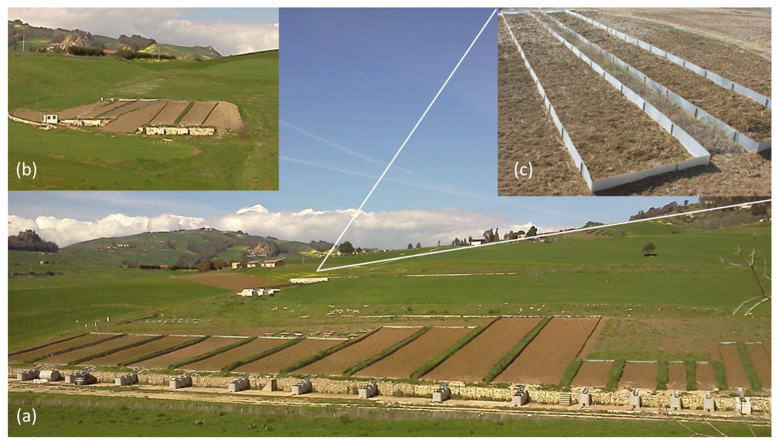
2.1. Experimental Plots and Datasets

| C-Db | I-Db | R-Db | ||||||||||||
|---|---|---|---|---|---|---|---|---|---|---|---|---|---|---|
| λ × w (m × m) | s (-) | Number of Plots | b1 | R2 | p | n | b1 | R2 | p | n | b1 | R2 | p | n |
| 22 × 2 | 0.09 | 2 | 1.173 | 0.53 | 0.0003 | 20 | 0.951 * | 0.31 | 0.0169 | 18 | ||||
| 11 × 2 and 11 × 4 | 0.149 | 4 | 1.398 | 0.54 | 0.0000 | 119 | 1.294 | 0.48 | 0.0000 | 102 | 1.046 | 0.74 | 0.0000 | 17 |
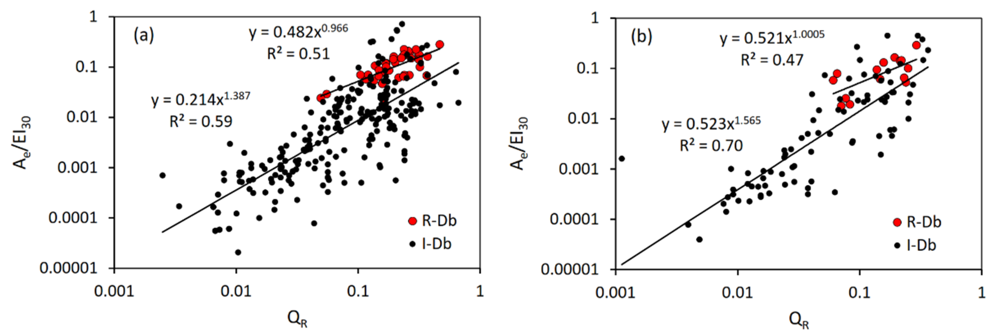
| 22 × 2 and 22 × 8 | 0.149 | 8 | 1.541 | 0.63 | 0.0000 | 282 | 1.388 | 0.59 | 0.0000 | 240 | 0.966 | 0.51 | 0.0000 | 42 |
| 33 × 8 | 0.149 | 2 | 1.650 | 0.72 | 0.0000 | 99 | 1.565 | 0.70 | 0.0000 | 84 | 1.000 | 0.47 | 0.0045 | 15 |
| 44 × 8 | 0.149 | 2 | 1.751 | 0.65 | 0.0000 | 63 | 1.665 | 0.60 | 0.0000 | 57 | 0.241 * | 0.05 | 0.672 | 6 |
| 22 × 6 | 0.22 | 2 | 1.208 | 0.43 | 0.0000 | 74 | 1.214 | 0.51 | 0.0000 | 53 | 0.832 | 0.36 | 0.0039 | 21 |
| 22 × 6 | 0.26 | 2 | 1.254 | 0.32 | 0.0000 | 63 | 1.310 | 0.35 | 0.0000 | 51 | 1.214 | 0.52 | 0.0079 | 12 |
| Database | Statistic | Pe | EI30 | QR | QREI30 | Ae |
|---|---|---|---|---|---|---|
| C-Db | min | 11.8 | 8.05 | 0.0011 | 0.058 | 0.0012 |
| max | 145.8 | 988.8 | 0.81 | 508.2 | 272.9 | |
| mean | 46.8 | 166.5 | 0.13 | 21.6 | 9.4 | |
| median | 41.6 | 104.9 | 0.09 | 11.3 | 1.5 | |
| CV | 0.60 | 0.93 | 0.93 | 1.7 | 2.3 | |
| I-Db | min | 11.8 | 8.05 | 0.0011 | 0.058 | 0.0012 |
| max | 145.8 | 469.8 | 0.74 | 71.0 | 92.5 | |
| mean | 48.6 | 134.3 | 0.11 | 12.6 | 4.0 | |
| median | 42 | 103.9 | 0.07 | 9.2 | 0.7 | |
| CV | 0.60 | 0.78 | 1.00 | 1.0 | 2.0 | |
| R-Db | min | 14.8 | 57.9 | 0.03 | 2.6 | 1.15 |
| max | 97.8 | 988.8 | 0.81 | 508.2 | 272.9 | |
| mean | 37.3 | 336.0 | 0.20 | 69.0 | 38.0 | |
| median | 33 | 265.3 | 0.18 | 41.3 | 27.5 | |
| CV | 0.46 | 0.73 | 0.57 | 1.0 | 1.1 |
2.2. Model Parameterization
2.3. Performance of the USLE-MB Model
3. Results
3.1. Rainfall–Runoff Erosivity Factor

3.2. Determination of the Soil Erodibility Factor and the Topographic Factors of the USLE-MB

3.3. Comparing USLE-MB Equations
4. Discussion
4.1. Rainfall–Runoff Erosivity Factor and Soil Erodibility Factor
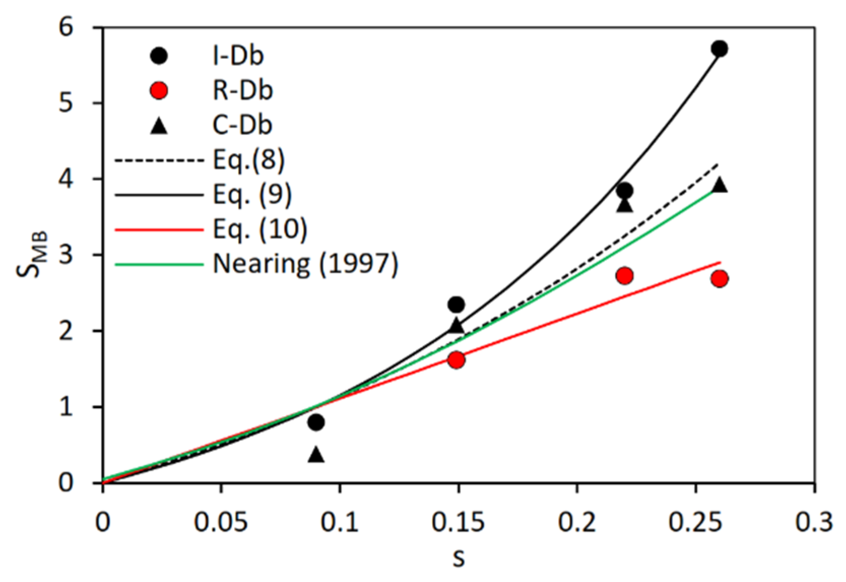
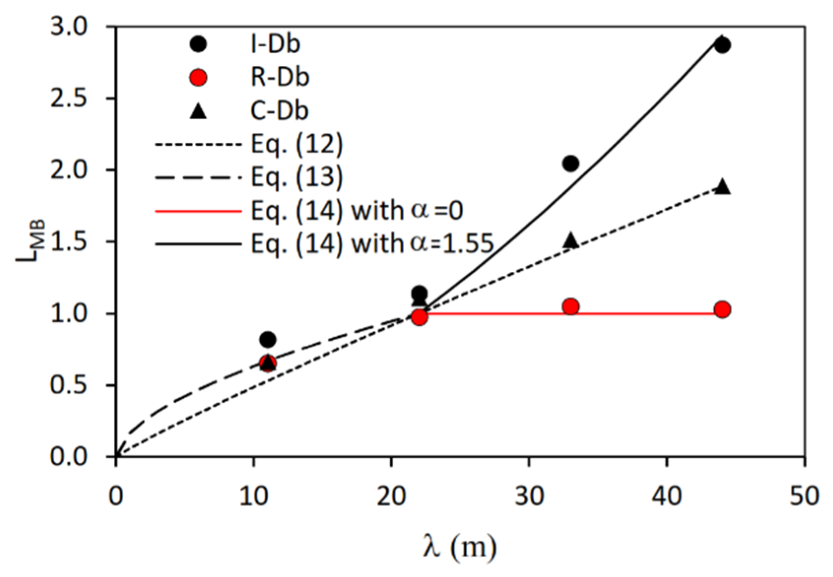
4.2. Topographic Factors

4.3. Comparing USLE-MB Equations
5. Conclusions
Author Contributions
Funding
Data Availability Statement
Conflicts of Interest
References
- Borrelli, P.; Robinson, D.A.; Fleischer, L.R.; Lugato, E.; Ballabio, C.; Alewell, C.; Meusburger, K.; Modugno, S.; Schütt, B.; Ferro, V.; et al. An assessment of the global impact of 21st century land use change on soil erosion. Nat. Commun. 2017, 8, 2013. [Google Scholar] [CrossRef] [PubMed] [Green Version]
- Di Stefano, C.; Ferro, V.; Pampalone, V. Modeling Rill Erosion at the Sparacia Experimental Area. J. Hydrol. Eng. 2015, 20, C5014001. [Google Scholar] [CrossRef]
- Di Stefano, C.; Ferro, V. Establishing soil loss tolerance: An overview. J. Agric. Eng. 2016, XLVII, 127–133. [Google Scholar] [CrossRef] [Green Version]
- Borrelli, P.; Robinson, D.A.; Panagos, P.; Lugato, E.; Yang, J.E.; Alewell, C.; Wuepper, D.; Montanarella, L.; Ballabio, C. Land use and climate change impacts on global soil erosion by water (2015–2070). Proc. Natl. Acad. Sci. USA 2020, 117, 21994–22001. [Google Scholar] [CrossRef] [PubMed]
- Panagos, P.; Borrelli, P.; Poesen, J.; Ballabio, C.; Lugato, E.; Meusburger, K.; Montanarella, L.; Alewell, C. The new assessment of soil loss by water erosion in Europe. Environ. Sci. Policy 2015, 54, 438–447. [Google Scholar] [CrossRef]
- Cerdan, O.; Govers, G.; Le Bissonnais, Y.; Van Oost, K.; Poesen, J.; Saby, N.; Gobin, A.; Vacca, A.; Quinton, J.; Auerswald, K.; et al. Rates and spatial variations of soil erosion in Europe: A study based on erosion plot data. Geomorphology 2010, 122, 167–177. [Google Scholar] [CrossRef]
- Nearing, M.A.; Foster, G.R.; Lane, L.J.; Finkner, S.C. A Process-Based Soil Erosion Model for USDA-Water Erosion Prediction Project Technology. Trans. ASAE 1989, 32, 1587–1593. [Google Scholar] [CrossRef]
- Morgan, R.P.C.; Quinton, J.N.; Smith, R.E.; Govers, G.; Poesen, J.W.A.; Auerswald, K.; Chisci, G.; Torri, D.; Styczen, M.E. The European soil erosion model (EUROSEM): A process-based approach for predicting soil loss from fields and small catchments. Earth Surf. Process. Landf. 1998, 23, 527–544. [Google Scholar] [CrossRef]
- Di Stefano, C.; Ferro, V.; Pampalone, V.; Sanzone, F. Field investigation of rill and ephemeral gully erosion in the Sparacia experimental area, South Italy. Catena 2013, 101, 226–234. [Google Scholar] [CrossRef]
- Rejman, J.; Brodowski, R. Rill characteristics and sediment transport as a function of slope length during a storm event on loess soil. Earth Surf. Process. Landf. 2005, 30, 231–239. [Google Scholar] [CrossRef]
- USDA. Revised Universal Soil Loss Equation Version 2 (RUSLE2); Science documentation; USDA-Agricultural Research Service: Washington, DC, USA, 2008.
- Tiwari, A.K.; Risse, L.M.; Nearing, M.A. Evaluation of WEPP and its comparison with usle and rusle. Trans. ASAE 2000, 43, 1129–1135. [Google Scholar] [CrossRef]
- Morgan, R.P.C.; Nearing, M.A. Handbook of Erosion Modelling; John Wiley and Sons: Hoboken, NJ, USA, 2011; pp. 1–401. [Google Scholar]
- Renard, K.G.; Foster, G.R.; Weesies, G.A.; McCool, D.K.; Yoder, D.C. Predicting Soil Erosion by Water: A Guide to Conservation Planning with the Revised Universal Soil Loss Equation (RUSLE). In USDA Agriculture Handbook, 703; USDA: Washington, DC, USA, 1997. [Google Scholar]
- Nearing, M.A. 22-Soil erosion and conservation. In Environmental Modelling: Finding Simplicity in Complexity, 2nd ed.; Wainwright, J., Mulligan, M., Eds.; John Wiley & Sons, Ltd.: Hoboken, NJ, USA, 2013; pp. 365–378. [Google Scholar]
- Alewell, C.; Borrelli, P.; Meusburger, K.; Panagos, P. Using the USLE: Chances, challenges and limitations of soil erosion modelling. Int. Soil Water Conserv. Res. 2019, 7, 203–225. [Google Scholar] [CrossRef]
- Batista, P.V.G.; Davies, J.; Silva, M.L.N.; Quinton, J.N. On the evaluation of soil erosion models: Are we doing enough? Earth Sci. Rev. 2019, 197, 102898. [Google Scholar] [CrossRef]
- McGehee, R.P.; Flanagan, D.C.; Srivastava, P.; Engel, B.A.; Huang, C.-H.; Nearing, M.A. An updated isoerodent map of the conterminous United States. Int. Soil Water Conserv. Res. 2022, 10, 1–16. [Google Scholar] [CrossRef]
- Kinnell, P.I.A.; Risse, L.M. USLE-M: Empirical Modeling Rainfall Erosion through Runoff and Sediment Concentration. Soil Sci. Soc. Am. J. 1998, 62, 1667–1672. [Google Scholar] [CrossRef]
- Kinnell, P. Event soil loss, runoff and the Universal Soil Loss Equation family of models: A review. J. Hydrol. 2010, 385, 384–397. [Google Scholar] [CrossRef]
- Bagarello, V.; Di Piazza, G.V.; Ferro, V.; Giordano, G. Predicting unit plot soil loss in Sicily, south Italy. Hydrol. Process. 2008, 22, 586–595. [Google Scholar] [CrossRef]
- Bagarello, V.; Ferro, V.; Pampalone, V. A new version of the USLE-MM for predicting bare plot soil loss at the Sparacia (South Italy) experimental site. Hydrol. Process. 2015, 29, 4210–4219. [Google Scholar] [CrossRef]
- Bagarello, V.; Di Stefano, C.; Ferro, V.; Pampalone, V. Comparing theoretically supported rainfall-runoff erosivity factors at the Sparacia (South Italy) experimental site. Hydrol. Process. 2018, 32, 507–515. [Google Scholar] [CrossRef]
- Di Stefano, C.; Pampalone, V.; Todisco, F.; Vergni, L.; Ferro, V. Testing the Universal Soil Loss Equation-MB equation in plots in Central and South Italy. Hydrol. Process. 2019, 33, 2422–2433. [Google Scholar] [CrossRef]
- Bagarello, V.; Ferro, V.; Flanagan, D. Predicting plot soil loss by empirical and process-oriented approaches. A review. J. Agric. Eng. 2018, 49, 1–18. [Google Scholar] [CrossRef]
- Di Stefano, C.; Palmeri, V.; Pampalone, V. An automatic approach for rill network extraction to measure rill erosion by ter-restrial and low-cost UAV photogrammetry. Hydrol. Process. 2019, 33, 1883–1895. [Google Scholar]
- Pampalone, V.; Carollo, F.G.; Nicosia, A.; Palmeri, V.; Di Stefano, C.; Bagarello, V.; Ferro, V. Measurement of Water Soil Erosion at Sparacia Experimental Area (Southern Italy): A Summary of More than Twenty Years of Scientific Activity. Water 2022, 14, 1881. [Google Scholar] [CrossRef]
- Wischmeier, W.H.; Smith, D.D. Predicting Rainfall-Erosion Losses—A Guide to Conservation Farming; USDA Agricultural Handbook no. 537; USDA: Blacksburg, VA, USA, 1978.
- Di Stefano, C.; Ferro, V.; Pampalone, V. Applying the USLE Family of Models at the Sparacia (South Italy) Experimental Site. Land Degrad. Dev. 2017, 28, 994–1004. [Google Scholar] [CrossRef]
- Nearing, M.A. A Single, Continuous Function for Slope Steepness Influence on Soil Loss. Soil Sci. Soc. Am. J. 1997, 61, 917–919. [Google Scholar] [CrossRef]
- Zhang, G.-H.; Liu, Y.-M.; Han, Y.-F.; Zhang, X.C. Sediment Transport and Soil Detachment on Steep Slopes: I. Transport Capacity Estimation. Soil Sci. Soc. Am. J. 2009, 73, 1291–1297. [Google Scholar] [CrossRef]
- Bagarello, V.; Di Stefano, C.; Ferro, V.; Giordano, G.; Iovino, M.; Pampalone, V. Estimating the USLE Soil Erodibility Factor in Sicily, South Italy. Appl. Eng. Agric. 2012, 28, 199–206. [Google Scholar] [CrossRef]
- Mutchler, C.K.; Carter, C.E. Soil Erodibility Variation During the Year. Trans. ASAE 1983, 26, 1102–1104. [Google Scholar] [CrossRef]
- Torri, D.; Borselli, L.; Guzzetti, F.; Calzolari, C.; Bazzoffi, P.; Ungaro, F.; Salvador Sanchis, M.P. Soil erosion in Italy: An overview. In Soil Erosion in Europe; Boardman, J., Poesen, J., Eds.; Wiley: New York, NY, USA, 2006; pp. 245–261. [Google Scholar]
- Zanchi, C. Soil loss and seasonal variation of erodibility in two soils with different texture in the Mugello valley in Central Italy. Catena Suppl. 1988, 12, 167–174. [Google Scholar]
- Boix-Fayos, C.; Calvo-Cases, A.; Imeson, A.C.; Soriano-Soto, M.D.; Tiemessen, I.R. Spatial and short-term temporal variations in runoff, soil aggregation and other soil properties along a Mediterranean climatological gradient. Catena 1998, 33, 123–138. [Google Scholar] [CrossRef]
- Boix-Fayos, C.; Calvo-Cases, A.; Imeson, A.C.; Soriano-Soto, M.D. Influence of soil properties on the aggregation of some Mediterranean soils and use of aggregate size and stability as land degradation indicators. Catena 2001, 44, 47–67. [Google Scholar] [CrossRef]
- Al-Durrah, M.; Bradford, J.M. New Methods of Studying Soil Detachment due to Waterdrop Impact. Soil Sci. Soc. Am. J. 1981, 45, 949–953. [Google Scholar] [CrossRef]
- Hussein, M.H.; Kariem, T.H.; Othman, A.K. Predicting soil erodibility in northern Iraq using natural runoff plot data. Soil Tillage Res. 2007, 94, 220–228. [Google Scholar] [CrossRef]
- Bagarello, V.; Ferro, V. Scale Effects on Plot Runoff and Soil Erosion in a Mediterranean Environment. Vadose Zone J. 2017, 16, 1–14. [Google Scholar] [CrossRef]
- Bagarello, V.; Ferro, V.; Pampalone, V. Testing assumptions and procedures to empirically predict bare plot soil loss in a Med-iterranean environment. Hydrol. Process. 2015, 29, 2414–2424. [Google Scholar] [CrossRef]
- Bagarello, V.; Ferro, V. Analysis of soil loss data from plots of differing length for the Sparacia experimental area, Sicily, Italy. Biosyst. Eng. 2010, 105, 411–422. [Google Scholar] [CrossRef]
- Bagarello, V.; Ferro, V.; Giordano, G.; Mannocchi, F.; Pampalone, V.; Todisco, F.; Vergni, L. Effect of plot size on measured soil loss for two Italian experimental sites. Biosyst. Eng. 2011, 108, 18–27. [Google Scholar] [CrossRef]
- Gao, G.Y.; Fu, B.J.; Lü, Y.H.; Liu, Y.; Wang, S.; Zhou, J. Coupling the modified SCS-CN and RUSLE models to simulate hydro-logical effects of restoring vegetation in the Loess Plateau of China. Hydrol. Earth Syst. Sci. Discuss. 2012, 16, 2347–2364. [Google Scholar] [CrossRef] [Green Version]
- Shi, W.; Huang, M.; Barbour, S.L. Storm-based CSLE that incorporates the estimated runoff for soil loss prediction on the Chinese Loess Plateau. Soil Tillage Res. 2018, 180, 137–147. [Google Scholar] [CrossRef]
- Todisco, F.; Brocca, L.; Mannocchi, F.; Melone, F.; Moramarco, T. Utilizzo di modellistica idrologica in continuo accoppiata ad un modello USLE modificato per la previsione della perdita di suolo parcellare in Umbria. Quad. Idronomia Mont. 2012, 30, 353–362, (In Italian with English Abstract). [Google Scholar]
- Todisco, F.; Vergni, L.; Vinci, A.; Pampalone, V. Practical thresholds to distinguish erosive and rill rainfall events. J. Hydrol. 2019, 579, 124173. [Google Scholar] [CrossRef]
Disclaimer/Publisher’s Note: The statements, opinions and data contained in all publications are solely those of the individual author(s) and contributor(s) and not of MDPI and/or the editor(s). MDPI and/or the editor(s) disclaim responsibility for any injury to people or property resulting from any ideas, methods, instructions or products referred to in the content. |
© 2023 by the authors. Licensee MDPI, Basel, Switzerland. This article is an open access article distributed under the terms and conditions of the Creative Commons Attribution (CC BY) license (https://creativecommons.org/licenses/by/4.0/).
Share and Cite
Pampalone, V.; Nicosia, A.; Palmeri, V.; Serio, M.A.; Ferro, V. Rill and Interrill Soil Loss Estimations Using the USLE-MB Equation at the Sparacia Experimental Site (South Italy). Water 2023, 15, 2396. https://doi.org/10.3390/w15132396
Pampalone V, Nicosia A, Palmeri V, Serio MA, Ferro V. Rill and Interrill Soil Loss Estimations Using the USLE-MB Equation at the Sparacia Experimental Site (South Italy). Water. 2023; 15(13):2396. https://doi.org/10.3390/w15132396
Chicago/Turabian StylePampalone, Vincenzo, Alessio Nicosia, Vincenzo Palmeri, Maria Angela Serio, and Vito Ferro. 2023. "Rill and Interrill Soil Loss Estimations Using the USLE-MB Equation at the Sparacia Experimental Site (South Italy)" Water 15, no. 13: 2396. https://doi.org/10.3390/w15132396