Short-Term Ocean Rise Effects on Shallow Groundwater in Coastal Areas: A Case Study in Juelsminde, Denmark

Abstract

Coastal areas situated at lower elevations are becoming more vulnerable to flooding as a result of the accelerating rise in the global sea level. As the sea level rises, so does the groundwater. Barriers designed to shield against marine flooding do not provide protection against flooding caused by rising groundwater. Despite the increasing threat of groundwater flooding, there is limited knowledge about the relationship between sea level rise and groundwater fluctuations. This hinders the ability to adequately consider sea level rise-induced groundwater flooding in adaptation initiatives. This study aims to investigate how local groundwater in Juelsminde, Denmark, responds to changes in sea level and to evaluate the predictability of these changes using a machine learning model. The influence of the sea on the shallow groundwater level was investigated using six groundwater loggers located between 45 and 210 m from the coast. An initial manual analysis of the data revealed a systematic delay in the rise of water levels from the coast to inland areas, with a delay of approximately 15–17 h per 50 m of distance. Subsequently, a support vector regression model was used to predict the groundwater level 24 h into the future. This study shows how the groundwater level in Juelsminde is affected by sea level fluctuations. The results suggest a need for increased emphasis on this topic.

1. Introduction

The global sea level rise is accelerating due to the melting of ice sheets and the thermal expansion of the oceans as a result of climate change [1,2,3]. This will affect millions of people living in low-lying coastal areas worldwide [1,4,5], and many urban coastal areas are already experiencing the consequences of increased precipitation, such as more frequent storm events and sea level rise (SLR) [6].

While SLR poses direct challenges to coastal areas, such as flooding and erosion [7,8,9], groundwater inundation (GWI) is an indirect and increasingly problematic consequence of SLR [8]. The groundwater level (GWL), especially in permeable ground, responds to tidal forces. This narrowing of the unsaturated space between the GWL and infrastructure may lead to GWI. Extremely high tides and SLR will intensify these floods due to a higher groundwater table and reduced unsaturated space to store water from storm events [6,10,11,12,13]. There may be many contributors that can influence GWI, such as rainfall, temperature, geology, and high tides during a storm event. Furthermore, low-lying coastal zones are prone to compound flooding, where marine and/or surface flooding can happen simultaneously with GWI [4,9]. Coastal barriers designed to protect against surface water are not effective in preventing flooding from below, making GWI especially problematic. This leaves buildings, basements, and both underground and surface infrastructure at risk of flooding [6,8,11,12,14,15]. Consequently, it can lead to contamination of the surface and groundwater with sewage [10].

The role of groundwater is important to fully understand the effect of SLR in coastal areas; however, it is often inadequately addressed in studies related to this topic. The effects of SLR are often assessed using numerical modelling, but there are few studies on the modelling and forecasting of GWI. This lack of information on GWI in coastal areas means that it is not being adequately considered in planning or adaptation initiatives [6,8,9,12,16]. Modelling GWI requires consideration of all parameters that may influence the GWL during extreme weather events, as well as the risk of compound flooding [9]. Thus far, many of the models used to investigate these systems have been based on physical principles. However, these models require substantial amounts of information about the system, and even when the data are available, they can be difficult to calibrate. Therefore, machine learning models are gaining popularity among hydrologists as screening tools or supplements to hydrological models, as they perform well and require less data input compared to the results they provide [6].

Existing research papers on the effects of SLR on GWL portray a variety of methods and perspectives, reflecting the complexity of the topic.

Habel et al. [10] used a groundwater flow model to assess the impact of SLR and high tides on GWI in Waikiki, Honolulu, Hawaii and concluded that an SLR of only approximately 1 m would result in a significant increase in the surface area experiencing GWI and its corresponding ramifications. Bjerklie et al. [12] also found that SLR causes groundwater rise (GWR). Using a 3D groundwater flow model, researchers discovered that in New Haven, Connecticut, a 0.91 m SLR scenario resulted in a corresponding 0.91 m increase in the near-coast GWL. Furthermore, the model indicated that even a GWL ranging from 5.2 to 7.3 m above sea level responded to the SLR. Results from Knott et al. [15] using a groundwater flow model showed that in coastal New Hampshire, USA, there is an estimated mean rise in GWL of 66% of SLR between 0 and 1 km from the coastline. Additionally, the study found that there is a response in GWL up to 5 km inland (3% of SLR) from the coastline. Similar among these three studies is the conclusion that the models must include more parameters and/or data to enhance their reliability [10,12,15].

In Bowes et al.’s [6] study, two machine learning models, namely, long-short-term memory (LSTM) and recurrent neural networks (RNNs), were investigated for their effectiveness in forecasting and modelling GWL in Norfolk, Virginia. A comparison of the models showed that LTSM networks are useful in real-time operational forecasts, and authors predict that GWL forecasting will become a valuable tool in the future management and modelling of coastal flooding.

Although the described studies have addressed this topic in different localities around the world, no systematic research has been conducted on the impact of SLR on GWL in Denmark.

Therefore, this study aimed to investigate how the local groundwater table responds to fluctuations in sea level and to uncover regional variations in the dependence on sea level and precipitation in the town Juelsminde in Denmark. Finally, the predictability of groundwater fluctuations was tested using a simple machine learning model based on the information mentioned above.

2. Materials and Methods

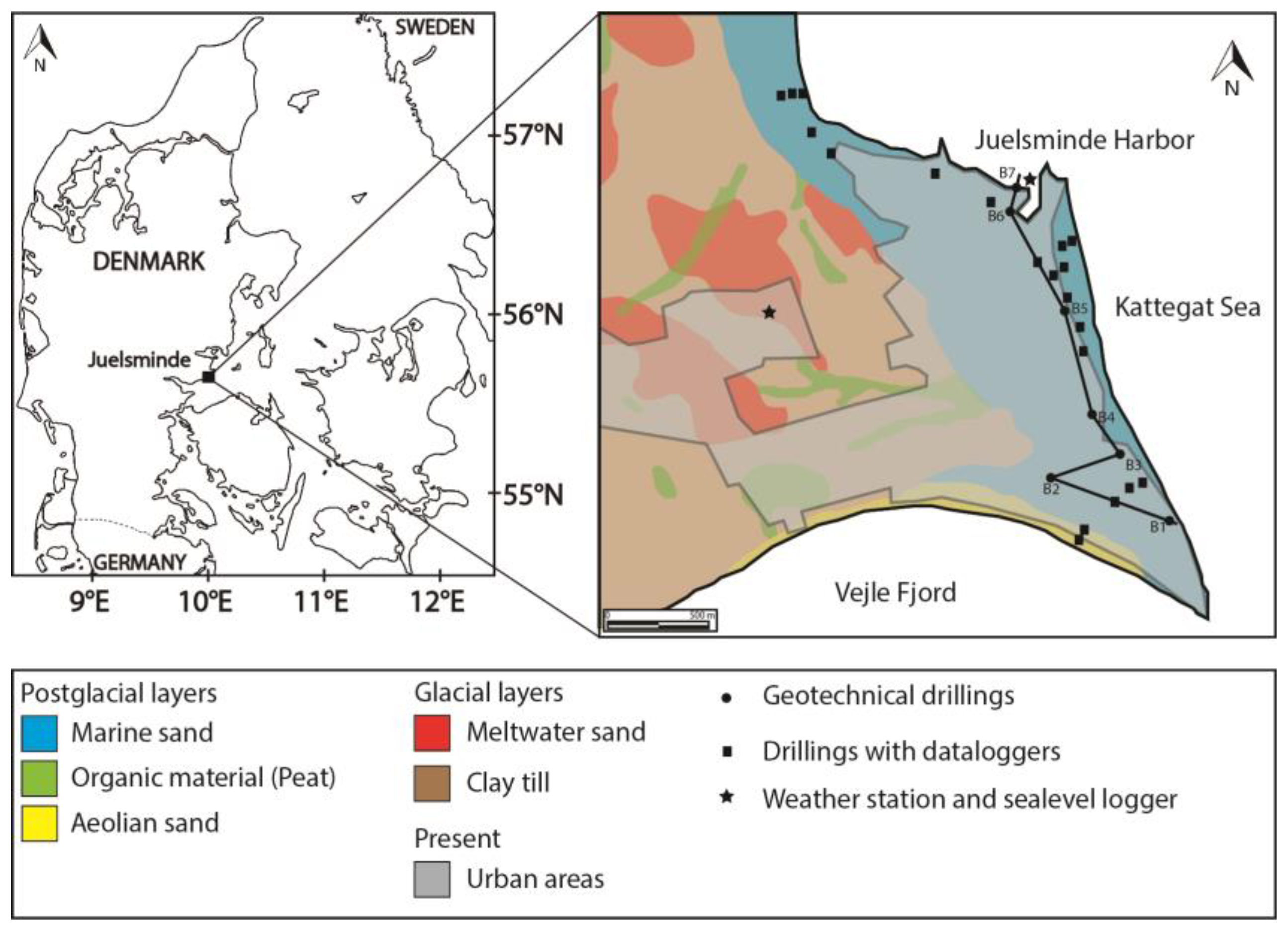
2.1. Study Area and Geological Setting

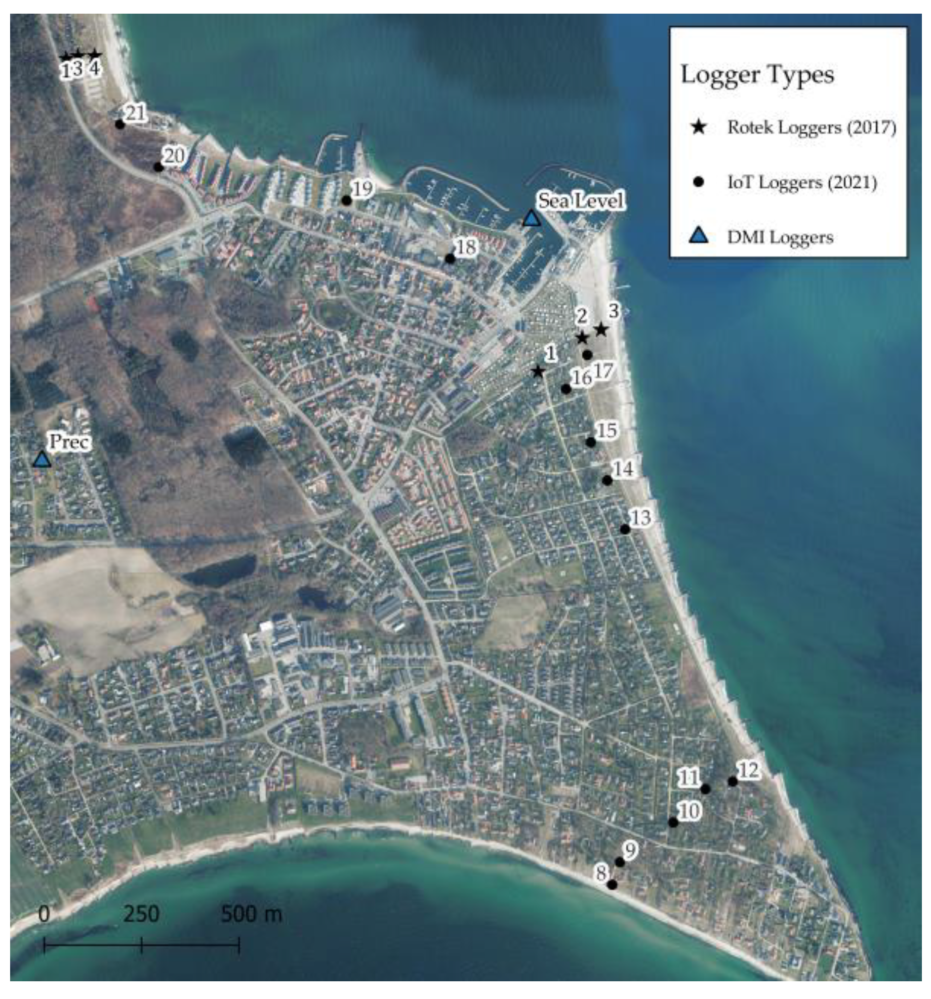
Juelsminde is located on the eastern coast of Jutland, Denmark, on a peninsula bordered by the Kattegat Sea to the east and Vejle Fjord to the south (Figure 1). Juelsminde is prone to flooding and has been identified as one of the top 10 cities in Denmark that are most at risk of flooding [17]. The nearshore areas are dominated by vacation homes, while the harbour is located in the northern part of the city. Further inland, residential houses dominate. A dike with an elevation of 2.6 m above sea level (masl) protects the buildings located south of the harbour from flooding caused by storm surges. The groundwater level is only 0–1 m below the ground surface (mbgs), and large parts of the city are drained through a series of ditches, from which water is pumped over the dike into the Kattegat Sea.

In Figure 1, the near-surface soil types are shown. The study area is characterised by glacial sediments in an elevated area to the west, covered by postglacial sediments in a lower lying area to the east. Figure 2 displays a geological cross-section based on well data. The glacial till observed in drilling B2 and located towards the west in Figure 1 was deposited during the Pleistocene glaciations, when the area was repeatedly covered by ice sheets [18]. The postglacial sediments are dominated by marine sand and, to a lesser extent, organic clay (Gyttja). The marine sand was deposited during the Holocene period, when ice melted and retreated, following the latest glaciation [19]. The sea level rose, causing low-lying areas in Denmark to flood based on the combined effect of the sea level rise and the land still being depressed from the weight of the ice sheets. The land has a much slower response to reaching equilibrium than the ocean. The flooding peaked during the Littorina transgression, which occurred approximately 8000 years ago [20]. This event is responsible for the lower marine sand layer observed in drilling B2. Marine conditions were established and the gyttja layer found in drilling B2 was deposited. The thickness of the lower marine sand is approximately 1 m, but it may be greater in areas where no organic clay is present. The organic clay layer has a thickness of 3 m and is composed of clay (Gyttja) containing plant remains and shells.

As the land rose following the ice retreat, the shoreline shifted towards its current position. During this regression, the upper layer of marine sand was deposited. It is up to 10 m thick and described as fine- to medium-grained, well-sorted sand containing shells.

The anthropogenic fillings in the area, typically 1–4 m thick, are expected to be local occurrences related to constructions and, as expected, the greatest thickness is found in the harbour area.

2.2. Data

Since 2017, six Rotek loggers have been measuring the GWL every 10 min, in addition to the manual measurements carried out every second week to validate the data. They are located along coast-perpendicular profiles, with distances from the coastline between 45 and 210 m (Figure 3).

The northernmost profile is located in an open area devoid of significant buildings, whereas the southern profile extends from the beach just south of the harbour and into the urbanised region behind the dike. In the last quarter of 2021, 14 additional IoT groundwater loggers were installed to investigate the dynamics along the coastline and gain a more comprehensive understanding of spatial variation. Tide gauges were installed along the coastline and in residential areas near the coast, as shown in Figure 3. The Danish Meteorological Institute (DMI) conducts sub-hourly measurements of the sea level in Juelsminde harbour. The precipitation amounts in Juelsminde are also recorded by the DMI. The data are freely available.

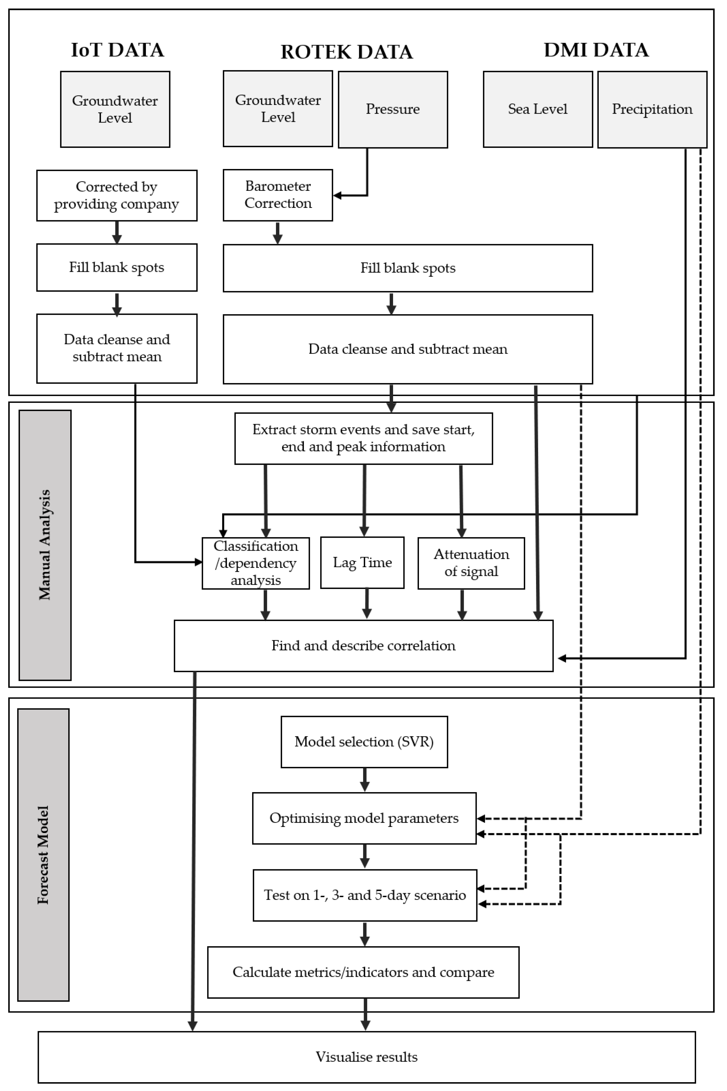
2.3. Data Preparation

The various sources of data require different levels of data processing, as shown in Figure 4. The data obtained from the six Rotek loggers were all corrected for barometric pressure. Where only a few values were missing, they were calculated using linear interpolation. Major outliers were removed (<0.02% of the dataset), and staggered sections were aligned with the rest of the data series. The sources of sudden jumps (offsets of sections) in the data are unknown, which means that there is a risk of correcting the wrong section of the data. This uncertainty is one of the reasons why this study focused on the relative changes in the groundwater table. The mean of the data series was subtracted, allowing easier comparison between the different groundwater time series. The data retrieved from the 14 IoT loggers were calibrated and referenced to the appropriate elevation below sea level (DVR90) [21], and significant outliers were removed by the company that, in addition, provided the groundwater loggers. The sea level and precipitation data from the DMI required very little correction. Only a few outliers were removed. All data series that were compared were first standardised to the same resolution before analysis, using either linear interpolation or downscaling.

In this study, two different analyses were carried out: (1) A manual analysis was conducted to examine the groundwater responses to high tide and storm events separately. Based on the results of the manual analysis, (2) a machine learning model was constructed to assess the predictability of the groundwater response.

Manual Analysis of the Sea Level and Groundwater Interaction

Rises in shallow groundwater levels resulting from large, sudden changes in sea level are typically more distinct and easier to identify and separate from each other than minor variations caused by tidal fluctuations. Additionally, they can be traced further inland, making them ideal for evaluating the systemic response of shallow groundwater to sea level rises. The most significant sea level rises were identified and extracted for analyses.

The analysis was conducted on the six data loggers (Rotek), with the longest available time series, placed in two profiles perpendicular to the coast. The sea level rise was determined by subtracting the mean sea level from the level recorded over the past two days. Through automated peak identification, time periods with a peak prominence over 1.2 m and an SL above 0.5 m were selected and are listed in

Table 1. An overview of the data sources used in this study.

Logger Type	Logger No.	Parameter	LON	LAT	Distance to Coast (m)	Start Time
Rotek loggers	1	Barometer	55.719466	9.997424	139	27 September 2017
	2	GWL	55.719519	9.997907	139	1 August 2018
	3	GWL	55.719519	9.998589	101	27 September 2017
	4	GWL	55.712096	10.01651	52,5	27 September 2017
	5	GWL	55.712857	10.018334	210	27 September 2017
	6	GWL	55.713039	10.019108	91	27 September 2017
	7	GWL	55.715592	10.016333	45,5	27 September 2017
IoT loggers	8	GWL	55.700241	10.019238	25	9 November 2021
	9	GWL	55.700759	10.019567	85	9 November 2021
	10	GWL	55.701656	10.021771	237	9 November 2021
	11	GWL	55.702416	10.023098	166	9 November 2021
	12	GWL	55.702576	10.024219	95	9 November 2021
	13	GWL	55.708428	10.019977	93	9 November 2021
	14	GWL	55.70956	10.019282	93	7 December 2021
	15	GWL	55.710447	10.018632	111	7 December 2021
	16	GWL	55.711681	10.01765	153	7 December 2021
	17	GWL	55.712459	10.018539	90	10 November 2021
	18	GWL	55.714725	10.012991	106	10 November 2021
	19	GWL	55.716101	10.008804	75	9 November 2021
	20	GWL	55.716932	9.999464	122	7 December 2021
	21	GWL	55.717932	10.001148	67	7 December 2021
DMI loggers	100	Sea level	55.7156	10.0163	-	27 September 2017
	101	Precipitation	55.7102	9.9962	-	27 September 2017

. Information regarding the scale of the SLR and the time interval covering the period of five days before the peak sea level and the subsequent seven days was gathered. This selection resulted in 30 high-tide events with relative amplitudes ranging from 1.22 to 1.96 m. An example of the automatic selection of high-sea-level events is shown in Figure 5.

A minimum threshold of 1.2 m for relative water level change ensures a high enough signal-to-noise ratio inland while also including a sufficient number of high-tide events to evaluate possible correlations. The process of peak selection and the subsequent analysis methods were inspired by Bowes et al. [6]. Modified versions of the available code were used. The resulting peak events are presented in

Table 2. The selected SLR events and the corresponding peak values.

Event No.	Start Datetime	Peak Datetime	End Datetime	Peak Prominence [cm]	SL at Peak (cm) (DVR90)
1	7 October 2017	13 October 2017	19 October 2017	131	79
2	13 October 2017	18 October 2017	25 October 2017	128	76
3	14 November 2017	19 November 2017	26 November 2017	131	88
4	6 December 2017	11 December 2017	18 December 2017	143	89
5	30 December 2017	4 January 2018	11 January 2018	138	87
6	11 January 2018	16 January 2018	23 January 2018	164	91
7	23 January 2018	28 January 2018	4 February 2018	135	74
8	7 February 2018	12 February 2018	19 February 2018	166	68
9	11 February 2018	16 February 2018	23 February 2018	142	60
10	22 February 2018	27 February 2018	6 March 2018	142	60
11	11 March 2018	16 March 2018	23 March 2018	142	60
12	13 November 2018	18 November 2018	25 November 2018	134	55
13	29 November 2018	4 December 2018	11 December 2018	175	109
14	3 January 2019	8 January 2019	15 January 2019	165	136
15	13 January 2019	18 January 2019	25 January 2019	124	74
16	6 February 2019	11 February 2019	18 February 2019	148	79
17	3 March 2019	8 March 2019	15 March 2019	162	104
18	11 March 2019	16 March 2019	23 March 2019	123	71
19	13 March 2019	18 March 2019	25 March 2019	134	76
20	10 September 2019	15 September 2019	22 September 2019	156	108
21	23 October 2019	28 October 2019	4 November 2019	123	79
22	24 November 2019	29 November 2019	6 December 2019	164	111
23	2 December 2019	7 December 2019	14 December 2019	122	102
24	7 December 2019	12 December 2019	19 December 2019	136	86
25	30 January 2020	4 February 2020	11 February 2020	139	93
26	4 February 2020	10 February 2020	16 February 2020	196	136
27	18 February 2020	23 February 2020	1 March 2020	149	102
28	8 March 2020	14 March 2020	20 March 2020	124	79
29	24 March 2020	29 March 2020	5 April 2020	124	75
30	11 September 2020	17 September 2020	23 September 2020	126	78

.

2.4. Response Time from the Sea Level Rise

To determine the lag time between the rise of the sea level and groundwater, an automated algorithm was used to calculate the time from the peak of the sea level rise to the peak of the groundwater level rise. Each storm event was analysed by extracting the time interval from both sea level and groundwater level data, with the sea level data being interpolated to match the higher resolution of the groundwater data. The raw data were compared to two filtered datasets using two different methods: (1) A Butterworth low-pass filter and (2) a running mean. These methods were employed to eliminate high frequencies, such as tidal changes, from the data. However, filtering affects the peak amplitude and, therefore, was only used to determine the signal delay. Applying a running mean proved to perform best on this dataset. The delay was found using cross-correlation of single loggers with the sea level data. All of the results were verified manually.

2.5. Attenuation of Groundwater Peak

The inland amplitude damping of the sea level rise indicates the extent to which a storm surge of a certain size affects the groundwater table. This attenuation was calculated for each event by determining the relative increase in the groundwater level at each logger location. The relative increase in GWL was calculated by subtracting the average GWL measured from 48 to 24 h prior to the GWL peak from the GWL at peak time.

2.6. Predictive Model

A delayed signal from the SLR and corresponding GWR enables the prediction of the GWL based on the sea level. The approach involved using a quick and simple model to gain insight into its predictive capabilities.

The primary objective of developing a predictive model is to estimate future increases in the groundwater level by considering current and forecasted changes in the sea level. The aim was to construct a model that could provide precise forecasts, and thus, the focus was primarily on calculating changes in the groundwater level one day in advance.

Based on initial tests using the same input in several simple machine learning models, support vector regression (SVR) provided the most accurate results. An SVR model is a regression model that determines the best fit based on a defined, acceptable error [22]. The model presented in this article is based on a linear kernel.

The model was partly based on historical data from the DMI and the monitored groundwater level data, with sea level and groundwater observations used as input. The DMI creates weather and sea level forecasts up to five days in advance. These forecasts can be utilised to generate predictions for the groundwater level, and based on these predictions, a warning system can be developed for areas at risk.

The model was trained on data from each of the six loggers individually, and the results were calculated separately for each logger. Hence, in this study, the model functioned as six separate models. The model’s predictive capabilities include 24 h, three-day, and five-day forecasts. The input parameters were selected in part based on the initial manual analysis of the data and the response of the groundwater.

In the final model, the input parameters were as follows:

• Groundwater level from the past four days;
• Sea level from the past four days and one day into the future (using the DMI’s one-day forecast);
• Precipitation from the past 24 h and one day into the future (using the DMI’s one-day forecast);
• Sine and cosine curve representing seasonality.

The model was trained on 60% of the available data, while the validation and cross-validation data each consisted of 20%.

The indicators’ adjusted R² (R²_adj) and predicted R² (R²_pred) were used to compare the model performance. R²_adj indicates how well the terms fit a curve or line, but it adjusts for the number of parameters in a model. This means that if a parameter is included in the model but does not contribute to the model, the R²_adj will decrease. If the parameter contributes to the model, R²_adj will increase. R²_adj will always be less than or equal to R². R² is the residual sum of squared errors divided by the total sum of squared errors.

$$R^2=1-\frac{S{S}_{RES}}{S{S}_{TOT}}=1-\frac{{{\displaystyle \sum }}_i{\left(y_i-{\widehat{y}}_i\right)}^2}{{{\displaystyle \sum }}_i{\left(y_i-{\overline{y}}_i\right)}^2}$$

(1)

where y_i is the dependent variable for observation i.

$$R_{adj}^2=1-\frac{\left(1-R^2\right)\left(n-1\right)}{n-k-1}$$

(2)

where n is the sample size and k is the number of variables in the model.

R²_pred is also known as the PRESS statistic and is used to determine how well a regression model makes predictions. If the data consist of a lot of noise, then R²_pred will be low, as it is not possible to predict random noise. R²_pred is useful to avoid overfitting.

$$R_{pred}^2=1-\left(\frac{PRESS}{S{S}_{TOT}}\right)=1-\frac{{{\displaystyle \sum }}_i{\left(y_i-{\hat{y}}_{\left(-i\right)}\right)}^2}{{{\displaystyle \sum }}_i{\left(y_i-{\overline{y}}_i\right)}^2}$$

(3)

where ${\hat{y}}_{\left(-i\right)}$ is the predicted value of the response variable for this observation found from the fitted regression equation [23,24].

3. Results and Discussion

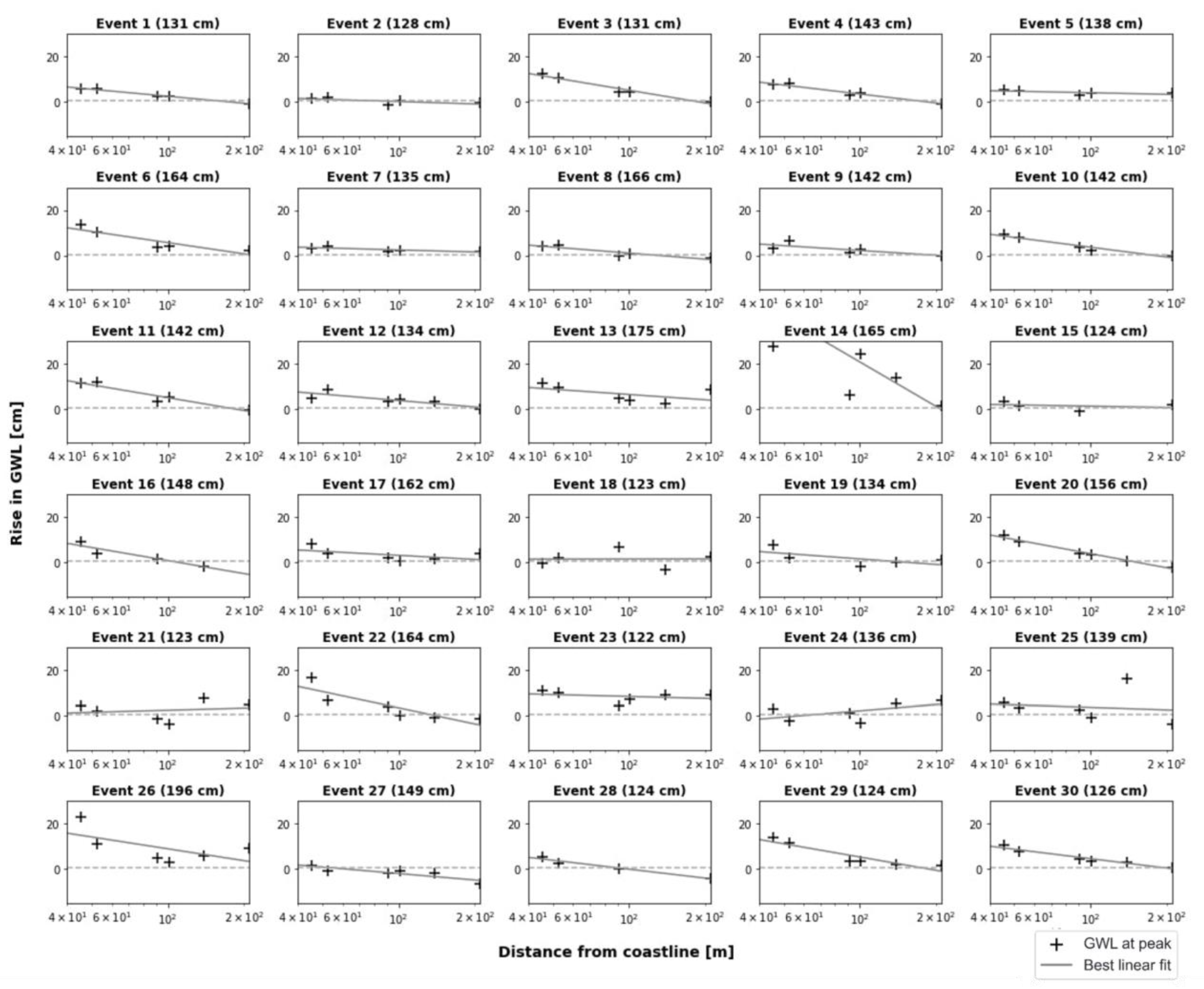
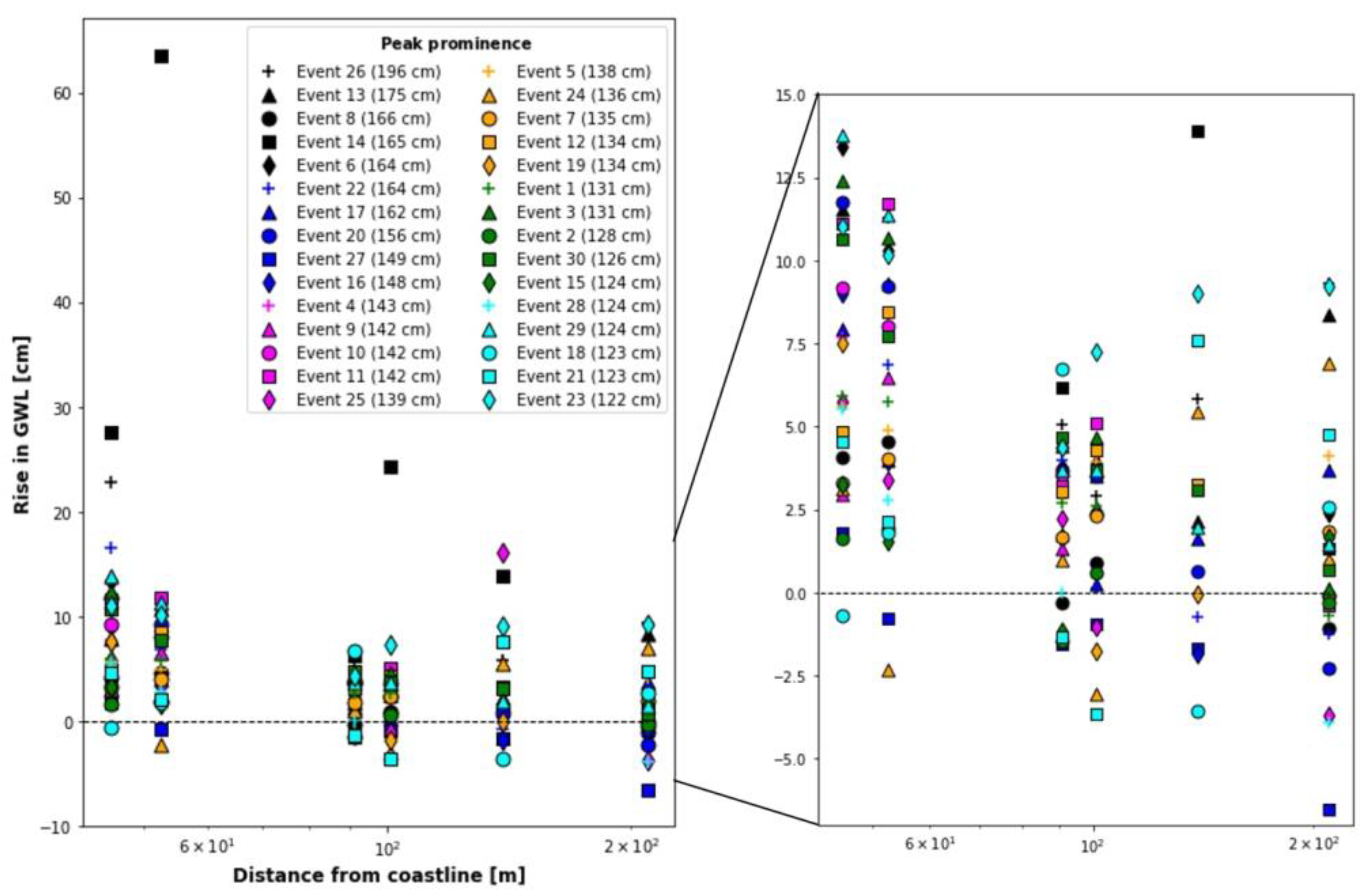
3.1. Groundwater Wave Characteristics

In a homogeneous medium, we expect to find a linear relationship between distance and time for the propagation of a wave peak. Figure 6 displays a boxplot representing the observed delay times at the loggers.

The loggers along the northern area, which are not affected by dikes or buildings, appeared to exhibit a linear relationship with a signal delay of approximately 14 h and 50 m to the coastline, reaching logger 2, 139 m from the coast, 25–26 h after the SLR. The two most coastal positions on the southern profile also appeared to reasonably follow the trend, while the farthest logger (logger 5) seemed to be influenced by other factors, with a delay time ranging between 25 and 30 h. This can be explained by the natural, high variation in the time lag response of the GWL, as the lag time is expected to be dependent on the magnitude of the sea level rise. The peak response in the GWL was clearly visible in the coastal loggers, but the algorithm had difficulty identifying the resulting rise in the loggers located further away from the coast. This is due to the low signal-to-noise ratio in the logger data, which made it difficult to identify. Moreover, the further inland the loggers are located, the greater the possibility that the signal from the SLR is drowned out by the responses from precipitation events. Furthermore, the further inland, the more likely that local pumping and drainage also affect the local groundwater level. It is worth noting that logger 5 is the only one placed on the inner side of the dike and within a constructed area. This may involve the presence of various low-conductivity barriers, which affect both the attenuation of the wave amplitude and delay the signal response in the groundwater well [25]. Consequently, this may account for the difficulty in detecting the signal in logger 5. Additionally, Sánchez-Úbeda et al. [26] suggested that the depth of the diver within the well can influence both the amplitude and the delay of the signal. In lower sections of the aquifer, the signal would experience less damping and travel at a faster pace. This observation is supported by previous studies [27,28]. In this study, the divers were located in the shallow aquifer, ranging from 121.4 cm (logger 6) to 297.8 cm (logger 5) in depth, with an average of 228 cm. Although the depth can potentially affect measurements, it is likely that this effect is more pronounced in deeper aquifers with higher pressure. Therefore, it is plausible that the low-conductivity layer associated with the dike or local infrastructure influenced the signal in well 5.

Figure 7 shows that the amplitude of the groundwater level decreased as the distance from the coast increased. We expect the amplitude damping in a free aquifer to follow a logarithmic function [29]. With a logarithmic time axis, the relationship could be estimated by fitting a straight line. However, there were outliers, especially when very large sea level rises occurred, resulting in extra-high amplitudes. Note that events 14 and 25 had outliers caused by possible mispicks. However, there were no sufficient arguments to exclude them from the dataset. A number of events (2, 7, 15, 18, and 21) exhibited no noteworthy increase in the GWL that could be attributed to the SLR. This may be due to a limited potential for a rise in the sea level. If an aquifer is limited by the topography, a groundwater table close to the terrain will leave little room to store more water and hence will not have the capacity to let the groundwater table rise in response to the sea level [30,31]. All of the events occurred in either October, January, or early March, which tend to be cold and wet months in Denmark [32]. Among these events, three (2, 18, and 19) experienced significantly above-average precipitation in either the previous or the current month, with September 2017 witnessing a 51% excess rainfall compared to the 1991–2020 average in Juelsminde, followed by a 128% deviation in March 2019 and a 62% deviation in October 2019 [33]. These excessive precipitation events may have caused the shallow groundwater to be so close to the terrain that it reached its topographic limitation. However, event 17, occurring just a week before event 18, produced a response in the groundwater loggers, despite similar topographic limitations. Event 17 exhibited a substantially higher SLR (162 cm) compared to event 18 (123 cm), ranking as the seventh highest and third lowest, respectively, among the listed events. Furthermore, the remaining four events without a response also fell within the lowest quarter (except event 7) when ordered by sea level rise (as depicted in Figure 8). This suggests that the currently defined lower threshold for significant sea level rises may be set too low, leading to the absence of a response in the groundwater level during these events.

Figure 8 displays the individual measurements from each event, sorted by the size of the SLR. The largest events generally showed the strongest responses in the GWL, but otherwise, there was no significant pattern amongst the smaller events. However, based on the observation made from Figure 7, eliminating the bottom 10 events may result in a cleaner dataset, revealing stronger correlations.

Figure 9 indicates a semi-linear relationship between the rise in sea level and the corresponding increase in the GWL. This relationship was particularly evident in the most prominent SLR events and in logger 7, which is closest to the coast. Although the relationship was also detectable in loggers 3 and 6, it was generally significantly less well defined in the two farthest loggers due to signal reduction. However, these trends are not entirely straightforward. There was significant variation among different events in terms of both the determination of phase shift and the change in amplitude. This is due to the simplification of the groundwater system in Juelsminde and the expectation of complete reliance on the ocean, particularly as the distance from the coast increases. The farther from the coast, the greater the influence of additional factors.

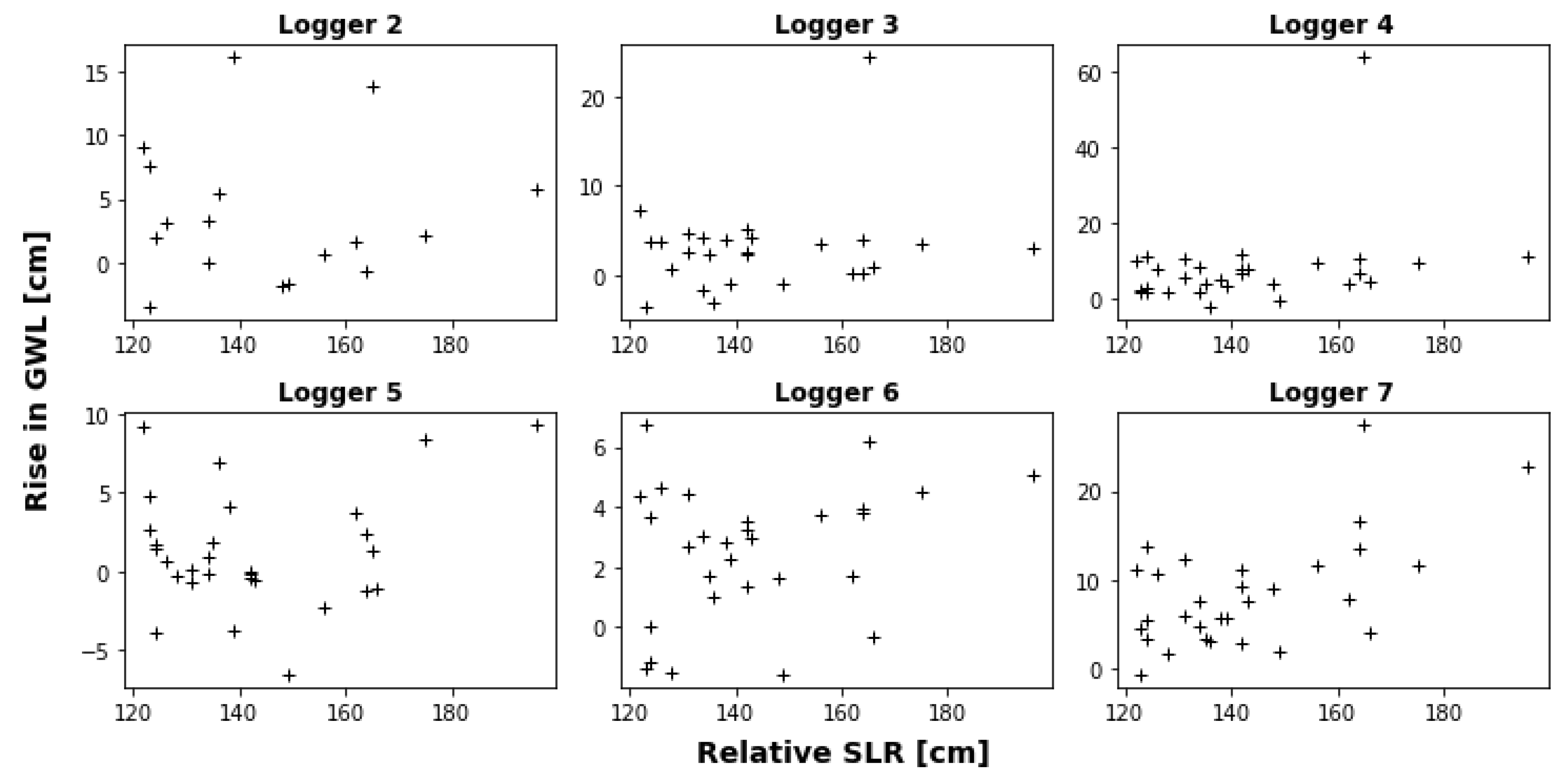
3.2. Sensitivity and Dependency Analysis

The 14 new loggers did not have time series long enough to contain sufficient events for the previous analysis. Instead, the data were used to conduct an overview analysis of the groundwater’s dependency on and sensitivity to sea level rises and precipitation events (Figure 10). The dependence on sea level fluctuations is determined not only by the storm surge responses, but also by the trace of tidal changes in the loggers. In these cases, precipitation has a reinforcing effect on the signal, but it is not the primary cause (blue circles). When the GWL cannot be correlated with sea level changes but mainly responds to precipitation, it belongs in the red (triangle) category. Half of the wells seemed to be equally influenced by the two parameters (black squares) and one logger provided too little data to categorise the well (white circle). In general, those loggers located closer to the coast tended to be more vulnerable to the impact of sea level changes compared to those situated further inland. In certain areas, this principle may not apply to individual loggers, and it is presumed that local conditions may influence which parameters have the greatest impact on the groundwater level in a logger. Hence, it may be difficult to determine exactly how much different parameters affect the various wells, but it can be generally stated that precipitation affects the GWL in all wells to varying degrees, while the impact of sea level is highly dependent on the distance to the coast. The sea level’s dependence is also an indication of the hydraulic connection between the well location and the ocean. Well no. 20 is located relatively far inland, but it clearly responds to tidal changes. It is located adjacent to a wetland that is connected to the ocean, which explains the rapid response. Well 14 appears to be primarily influenced by precipitation, despite no significant distinctions in its location compared to the neighbouring loggers 13 and 15. The cause of this discrepancy could be caused by either geological factors or local infrastructure. It is possible that there is an obstruction along the pathway from the coast to well 14, hindering the hydraulic connection. Alternatively, the contribution from precipitation in that specific area may be notably higher, leading to a greater accumulation of surface water. The abrupt transition from the blue to orange categories between loggers 8 and 9, as well as between 12 and 11, could be a result of topographical variations or the presence of infrastructure. Logger 8, located in close proximity to the shoreline and at a low elevation, might be affected by both topography and potential obstructions caused by infrastructure. Logger 9, situated within a built-up area, could experience a blockage in its hydraulic connection to the ocean or gather more surface water during precipitation events due to local construction. Logger 12 is positioned in an area with few buildings and no roads obstructing the path to the ocean. On the contrary, logger 11, located nearby, is surrounded by houses, which seemingly has a considerable impact. Further investigation into the types of infrastructure that have the greatest influence on sensitivity to precipitation and sea level rise would be of interest.

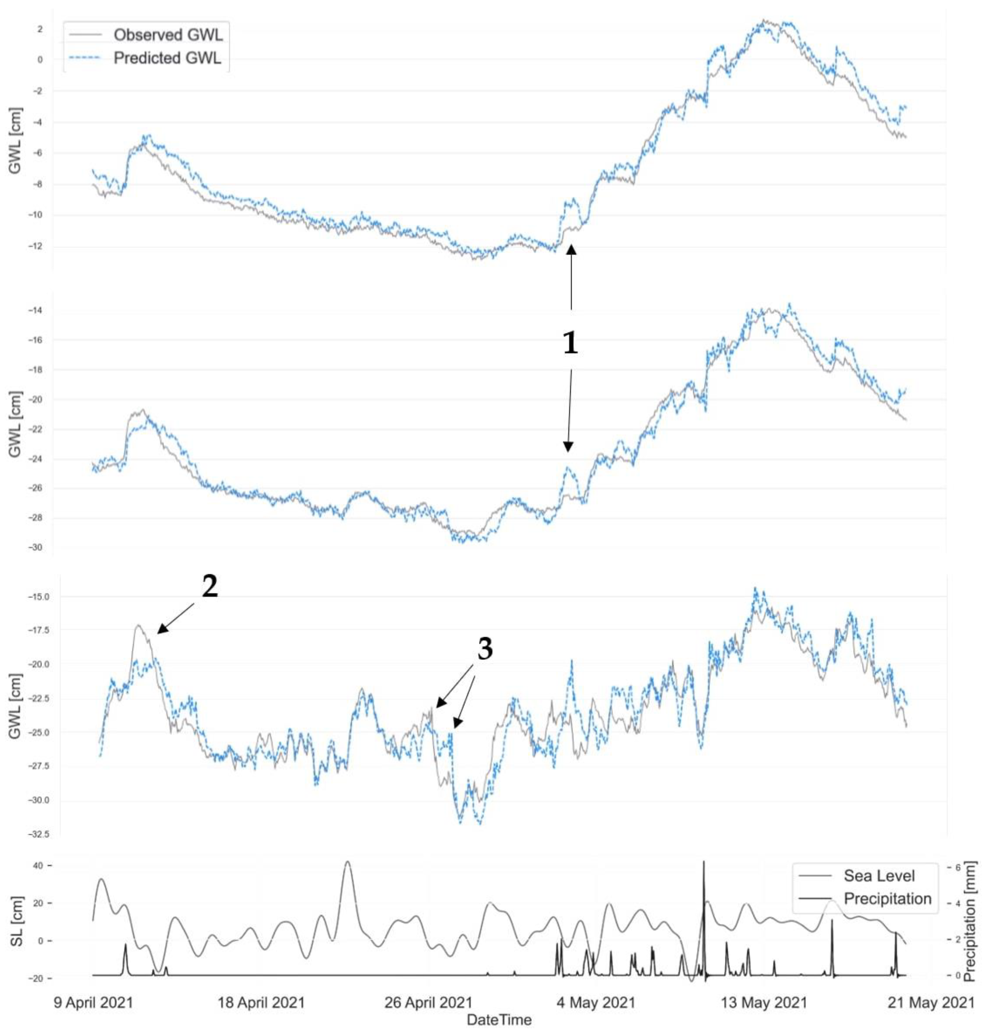
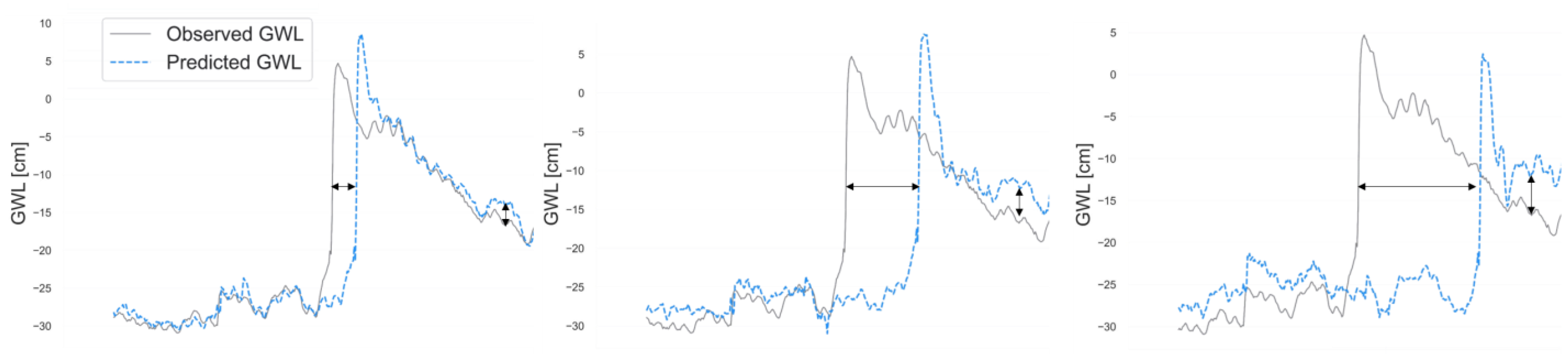
3.3. Predictability of Groundwater Fluctuations

Results from the 24 h predictions for wells 2–4 are displayed in Figure 11, with the distance to the coast increasing downwards. The time period depicted covers a high-water event and the consequent rise in GWL in the six wells.

The average correlation coefficient for this high-water event was approximately 90%, which indicates the percentage of variations that can be accounted for by the model. The model also performed well, with a high accuracy rate of 78%, in predicting the groundwater level. The average mean deviation was just below 1 cm.

The model, however, has its challenges. Three of the major issues are: (1) An overestimation of the contribution of precipitation; (2) challenges in predicting the extent of extreme GWL rises; (3) relying heavily on the previous groundwater measurements to calibrate the level in the current well. Overestimating the effect of precipitation on the signal can result in periods of a few hours, with significantly higher modelled values than those observed. On the contrary, the inability to model extreme events resulted in modelled values that were lower than the observed values. Both of these factors resulted in a significant deviation between the predicted and measured GWL. The reliability on previous measurements resulted in delayed replications of sudden changes and adjusted the level retroactively.

Table 3. The main outcomes of the SVR model predictions of the groundwater level 1, 3 and 5 days ahead using data from logger 4.

	1 Day		3 Days		5 Days
	Average	Std. Dev.	Average	Std. Dev.	Average	Std. Dev.
R2adj	0.76	0.19	0.43	0.37	−0.27	0.78
R2pred	0.10	0.99	0.23	0.51	−0.65	1.12
MAE	1.30	0.56	3.14	1.06	4.90	1.67
RMSE	1.99	1.07	6.94	2.45	13.02	4.29

provides a brief summary of the model’s overall performance in predicting changes in the groundwater level, specifically for one, three, and five days ahead. The R²_adj values showed that the modelled groundwater level corresponded well with the observed levels, but there were still difficulties with making independent predictions (R²_pred). The average deviation from the observed values was only a few centimetres. When attempting to predict groundwater changes three days into the future, the R²_adj decreased, while the ability to make accurate predictions (R²_pred) increased. This may be because the model was originally slightly overfitted, resulting in a greater deviation from the observed data but a less-constrained fit of the model when calculating the predicted values.

Based on Table 3, it seems unlikely that the model can generate valuable outcomes when trying to forecast groundwater fluctuations five days ahead. Here, both correlation coefficients were negative. However, plotting the model results for the same interval as presented in Figure 11 indicates a different outcome (Figure 12). Despite the greater disparities between the modelled groundwater table and the observed data, the model successfully captured the primary patterns.

The poor performance of the model, as indicated in Table 3, raises the question: Why does it exhibit such bad performance? One possible explanation can be observed in Figure 13, which depicts a notable and sudden rise in the groundwater level. The model struggled to foresee this abrupt change, resulting in a delayed signal in the predicted groundwater level. As the predictions extended further into the future, the discrepancy between the measured and predicted peaks widened, leading to a decrease in the adjusted correlation coefficient (R²_adj). Moreover, the model encountered difficulties in accurately maintaining the average groundwater level over time, causing it to deviate from the true water table. The segment illustrated in Figure 13 serves as an example, among several other instances, that contributes to the reduction of correlation coefficients and the amplification of mean errors. However, this does not imply that the model lacks value; instead, it emphasises the significance of identifying the sources behind any statistical deviations that appear unusual. In this specific case, it may be necessary to investigate whether the sudden increase in the groundwater level is driven by natural factors or human intervention, or whether it requires correction during the data processing stage.

4. Conclusions

Comparing sea level and groundwater data demonstrated a need for greater emphasis on addressing the flooding caused by groundwater following rises in the sea level—especially in countries with extensive coastlines and low-lying coastal infrastructure. Although the impact of a storm surge is most noticeable in those wells located closest to the coast, responses to the strongest storm surges were additionally registered in those wells furthest away. When there was a clear linear correlation between the delay time and the distance to the coast in an open, undisturbed area, the presence of built constructions appeared to obstruct the signal and cause a further delay.

The response signal experienced a delay that ranges from 14 h and 45 m near the coast to more than 30 h 210 m away from the coast. In several cases, it was difficult to identify the high-water signal in the loggers located far inland, possibly because the signal weakens logarithmically as it moves away from the coast. This causes the impact of factors such as rainfall to become significant enough to have a comparable amplitude, masking the signal from the sea. Meanwhile, a categorisation of the wells suggested that the groundwater level closer to the coast or with a well-established hydraulic connection to the ocean is more heavily influenced by the impact of the sea. Built areas proved to have a significant influence of the signal measured in the groundwater table, either due to low-conductivity barriers or an increased sensitivity to rainwater. In the single wells, there was a semi-linear correlation between the magnitude of the SLR and the corresponding rise in the groundwater table. The events with the smallest rise in sea level caused no or little response in the groundwater wells.

The delayed response allowed for the calculation of a predicted increase in the shallow groundwater subsequent to a sea level rise. The support vector regression model showed promising results when predicting the groundwater response in a logger 24 h in advance using sea level and rainfall data. While the modelled values of the three- and five-day predictions showed little deviation from the observed groundwater table, and single sections of sudden changes in groundwater level resulted in negative correlation coefficients. It would be interesting to introduce further improvements and move from single-step prediction to predicting entire time sequences. Additionally, expanding the model to a multi-output model calculating the groundwater table in all wells simultaneously would eliminate the need for calibrating each well.

This study highlighted the significance of incorporating the influence of sea level on groundwater variations in the development of predictive models and the examination of future groundwater levels. In certain regions, the interaction between the sea and the shallow groundwater table is intensifying, underscoring the relevance of including this factor in analyses. Furthermore, when determining appropriate climate adaptation strategies, it is crucial to account for the natural dynamics associated with these phenomena.

References

1. IPPC. Sea Level Rise and Implications for Low-Lying Islands, Coasts and Communities. In Special Report on the Ocean and Cryosphere in a Changing Climate, 1st ed.; Contribution of Working Group II to Technical Support, Unit; Pörtner, H.O., Roberts, D.C., Masson-Delmotte, V., Zhai, P., Tignor, M., Poloczanska, E., Mintenbeck, K., Alegría, A., Nicolai, M., Okem, A., et al., Eds.; Cambridge University Press: Cambridge, UK, 2019; pp. 321–447. [Google Scholar]
2. NOAA. Global and Regional Sea Level Rise Scenarios for the United States: Updated Mean Projections and Extreme Water Level Probabilities Along U.S. Coastlines. In 2022 Sea Level Rise Technical Report, 1st ed.; Sweet, W.V., Hamlington, B.D., Kopp, R.E., Weaver, C.P., Barnard, P.L., Bekaert, D., Brooks, W., Craghan, M., Dusek, G., Frederikse, T., et al., Eds.; National Oceanic and Atmospheric Administration, National Ocean Service: Silver Spring, MD, USA, 2022; p. 111. [Google Scholar]
3. Davtalab, R.; Mirchi, A.; Harris, R.J.; Troilo, M.X.; Madani, K. Sea Level Rise Effect on Groundwater Rise and Stormwater Retention Pond Reliability. Water 2020, 12, 1129. [Google Scholar] [CrossRef] [Green Version]
4. Sangsefidi, Y.; Bagheri, K.; Davani, H.; Merrifield, M. Data Analysis and Integrated Modeling of Compound Flooding Impacts on Coastal Drainage Infrastructure under a Changing Climate. J. Hydrol. 2023, 616, 128823. [Google Scholar] [CrossRef]
5. Robinson, C.E.; Xin, P.; Santos, I.R.; Charette, M.A.; Li, L.; Barry, D.A. Groundwater Dynamics in Subterranean Estuaries of Coastal Unconfined Aquifers: Controls on Submarine Groundwater Discharge and Chemical Inputs to the Ocean. Adv. Water Resour. 2018, 115, 315–331. [Google Scholar] [CrossRef]
6. Bowes, B.D.; Sadler, J.M.; Morsy, M.M.; Behl, M.; Goodall, J.L. Forecasting Groundwater Table in a Flood Prone Coastal City with Long Short-Term Memory and Recurrent Neural Networks. Water 2019, 11, 1098. [Google Scholar] [CrossRef] [Green Version]
7. Knott, J.F.; Elshaer, M.; Daniel, J.S.; Jacobs, J.M.; Kirshen, P. Assessing the Effects of Rising Groundwater from Sea Level Rise on the Service Life of Pavements in Coastal Road Infrastructure. Transp. Res. Rec. J. Transp. Res. Board 2017, 2639, 1–10. [Google Scholar] [CrossRef] [Green Version]
8. Habel, S.; Fletcher, C.H.; Rotzoll, K.; El-Kadi, A.I.; Oki, D.S. Comparison of a Simple Hydrostatic and a Data-Intensive 3D Numerical Modeling Method of Simulating Sea-Level Rise Induced Groundwater Inundation for Honolulu, Hawai’i, USA. Environ. Res. Commun. 2019, 1, 041005. [Google Scholar] [CrossRef]
9. Bosserelle, A.L.; Morgan, L.K.; Hughes, M.W. Groundwater Rise and Associated Flooding in Coastal Settlements Due to Sea-Level Rise: A Review of Processes and Methods. Earths Future 2022, 10, e2021EF002580. [Google Scholar] [CrossRef]
10. Habel, S.; Fletcher, C.H.; Rotzoll, K.; El-Kadi, A.I. Development of a Model to Simulate Groundwater Inundation Induced by Sea-Level Rise and High Tides in Honolulu, Hawaii. Water Res. 2017, 114, 122–134. [Google Scholar] [CrossRef]
11. Hoover, D.J.; Odigie, K.O.; Swarzenski, P.W.; Barnard, P. Sea-Level Rise and Coastal Groundwater Inundation and Shoaling at Select Sites in California, USA. J. Hydrol. Reg. Stud. 2017, 11, 234–249. [Google Scholar] [CrossRef] [Green Version]
12. Bjerklie, D.M.; Mullaney, J.R.; Stone, J.R.; Skinner, B.J.; Ramlow, M.A. Preliminary Investigation of the Effects of Sea-Level Rise on Groundwater Levels in New Haven, Connecticut, 1st ed.; U.S. Geological Survey: Reston, VA, USA, 2012; pp. 1–46. [Google Scholar]
13. Trglavcnik, V.; Morrow, D.; Weber, K.P.; Li, L.; Robinson, C.E. Analysis of Tide and Offshore Storm-Induced Water Table Fluctuations for Structural Characterization of a Coastal Island Aquifer. Water Resour. Res. 2018, 54, 2749–2767. [Google Scholar] [CrossRef] [Green Version]
14. Habel, S.; Fletcher, C.H.; Anderson, T.R.; Thompson, P.R. Sea-Level Rise Induced Multi-Mechanism Flooding and Contribution to Urban Infrastructure Failure. Sci. Rep. 2020, 10, 3796. [Google Scholar] [CrossRef] [PubMed] [Green Version]
15. Knott, J.F.; Jacobs, J.M.; Daniel, J.S.; Kirshen, P. Modeling Groundwater Rise Caused by Sea-Level Rise in Coastal New Hampshire. J. Coast. Res. 2019, 35, 143–157. [Google Scholar] [CrossRef]
16. Cooper, H.M.; Zhang, C.; Selch, D. Incorporating Uncertainty of Groundwater Modeling in Sea-Level Rise Assessment: A Case Study in South Florida. Clim. Chang. 2015, 129, 281–294. [Google Scholar] [CrossRef]
17. Kystdirektoratet. Revurdering og Ajourføring af Risikoområder for Oversvømmelse fra Hav og Vandløb. Oversvømmelsesdirektivet, Anden Planperiode, 1st ed.; Kystdirektoratet: Lemvig, Denmark, 2018; p. 38. [Google Scholar]
18. Houmark-Nielsen, M. Pleistocene stratigraphy and glacial history of the central part of Denmark. Bull. Geol. Soc. Denmark 1987, 36, 1–189. [Google Scholar] [CrossRef]
19. Houmark-Nielsen, M. The Pleistocene of Denmark: A review of stratigraphy and glaciation history. Dev. Quat. Sci. 2004, 2, 35–46. [Google Scholar] [CrossRef]
20. Stattegger, K.; Leszczyńska, K. Rapid sea-level rise during the first phase of the Littorina transgression in the western Baltic Sea. Oceanologia 2023, 65, 202–210. [Google Scholar] [CrossRef]
21. Vejledning om Højdesystemet. Available online: https://www.retsinformation.dk/eli/mt/2005/2 (accessed on 19 June 2023).
22. Géron, A. Support Vector Machines. In Hands-On Machine Learning with Scikit-Learn, Keras & TenserFlow—Concepts, Tools, and Techniques to Build Intellegent Systems, 2nd ed.; Butterfield, N., Taché, N., Cronni, M., Kelly, B., Cofer, K., Eds.; O’Reilly Media, Inc.: Sebastopol, CA, USA, 2019. [Google Scholar]
23. Dodge, Y. The Consise Encyclopedia of Statistics, 1st ed.; Springer: New York, NY, USA, 2008; pp. 1–583. [Google Scholar]
24. Everitt, B.S.; Skrondal, A. The Cambridge Dictionary of Statistics, 4th ed.; Cambridge University Press: Cambridge, UK, 2010. [Google Scholar]
25. Slooten, L.; Carrera, J.; Castro, E.; Fernàndez-Garcia, D. A Sensitivity Analysis of Tide-Induced Head Fluctuations in Coastal Aquifers. J. Hydrol. 2010, 393, 370–380. [Google Scholar] [CrossRef]
26. Sánchez-Úbeda, J.P.; Calvache, M.L.; López-Chicano, M.; Duque, C. The effect of non-tidal components, the use of peak delays, and depth of measurement for the application of tidal response methods. Water Resour. Manag. 2018, 32, 481–495. [Google Scholar] [CrossRef]
27. Erskine, A. The effect of tidal fluctuation on a coastal aquifer in the UK. Ground Water 1991, 29, 556–562. [Google Scholar] [CrossRef]
28. Levanon, E.; Shalev, E.; Yechieli, Y.; Gvirtzman, H. Fluctuations of fresh-saline water interface and of water table induced by sea tides in unconfined aquifers. Adv. Water Resour. 2016, 96, 34–42. [Google Scholar] [CrossRef]
29. Schwarts, F.W.; Zhang, H. Response of an Unconfined Aquifer to Pumping. In Fundamentals of Groundwater; Flahive, R., Powell, D., Eds.; John Wiley and Sons: New York, NY, USA, 2003; pp. 258–273. [Google Scholar]
30. Duque, C.; Meyer, R.; Sonnenborg, T.O. Saltwater intrusion in Denmark. Boletín Geológico Min. 2022, 133, 29–46. [Google Scholar] [CrossRef]
31. Michael, H.A.; Russoniello, C.J.; Byron, L.A. Global assessment of vulnerability to sea-level rise in topography-limited and recharge-limited coastal groundwater systems. Water Resour. Res. 2013, 49, 2228–2240. [Google Scholar] [CrossRef]
32. Climate Change Knowledge Portal—Denmark. Available online: https://climateknowledgeportal.worldbank.org/country/denmark/climate-data-historical (accessed on 16 June 2023).
33. Tabeller—Måned—DMI. Available online: https://www.dmi.dk/vejrarkiv/manedens-sasonens-og-arets-vejr/tabeller-maned/ (accessed on 16 June 2023).
Figure 1. Overview map showing the Juelsminde area, the soil types, the position of the wells and geotechnical drillings in Figure 2, and the location of the dataloggers.
Water 15 02425 g001
Figure 2. Cross-section through Juelsminde showing borehole lithologies.
Water 15 02425 g002
Figure 3. Location of the different logger types installed in the Juelsminde area.
Water 15 02425 g003
Figure 4. Workflow of the data treatment, analysis, and model process. The dashed arrows representing the data used for the forecast model.
Water 15 02425 g004
Figure 5. An example of the automatic selection of high-sea-level events. The blue crosses represent peak levels exceeding the minimum criteria.
Water 15 02425 g005
Figure 6. Boxplot (with medians marked in orange and 25% and 75% quartiles) visualising the lag times for the delayed responses in the groundwater table initiated by a sudden rise in the sea level in the northern (black) and the southern (grey) profiles.
Water 15 02425 g006
Figure 7. The relative rise in the ground-water level monitored in the wells for each of the 30 SLR events.
Water 15 02425 g007
Figure 8. The relative rise in groundwater level registered in the wells during 30 SLR events sorted by the peak prominence of the SLR event.
Water 15 02425 g008
Figure 9. The relative rise in the GWL plotted against the SLR peak prominence for all SLR events in the six wells from 2017.
Water 15 02425 g009
Figure 10. The classification results for the GWL in each well depending on the SLR or precipitation event.
Water 15 02425 g010
Figure 11. The modelled and observed GWL in wells 2 (top), 3 (middle), and 4 (bottom) during SLR and precipitation events. The number 1–3 represent the listed challenges of the model.
Water 15 02425 g011
Figure 12. The modelled results for 3- and 5-day predictions in logger 4.
Water 15 02425 g012
Figure 13. The modelled result for 1-, 3- and 5-day predictions during the event of an abrupt increase in the groundwater table. The arrows mark the increasing delay and shift of the model predictions.
Water 15 02425 g013