Modeling BTEX Multiphase Partitioning with Soil Vapor Extraction under Groundwater Table Fluctuation Using the TMVOC Model

Abstract

The effects of groundwater table fluctuation (GTF) on the remediation of a petrochemically polluted riverside using soil vapor extraction (SVE) were investigated. The migration and transformation of benzene, toluene, ethylbenzene, and o-xylene (BTEX) in cases of natural attenuation, SVE without GTF, and SVE with GTF were simulated using the TMVOC model. The results showed that the optimized extraction well pressure and influencing radius of the target site were 0.90 atm and 8 m, respectively. The removal rates of BTEX in cases of natural attenuation, SVE without GTF, and SVE with GTF were 11.49%, 85.16%, and 97.33%, respectively. The removal rate of BTEX was maximized in the case of SVE with a GTF amplitude of 0.5 m to 1 m. The removal rates of benzene (99.99%), toluene (99.74%), ethylbenzene (96.37%), and o-xylene (94.72%) were maximized in the case of SVE with GTF. For the cases of SVE without GTF and SVE with GTF, mass losses of BTEX in gaseous (0.05 kg, 0.05 kg, respectively) and aqueous phases (5.46 kg, 5.87 kg, respectively) were consistent. However, the mass loss of BTEX in the non-aqueous phase liquid (NAPL) phase in the case of SVE with GTF (155.13 kg) exceeded that in the case of SVE without GTF (135.41 kg). This is because GTF positively affected both the solubility and volatility of BTEX in the NAPL phase. With the groundwater table decreasing, flows of gas and gaseous pollutants increased by 25% along the vertical section. At this stage, the removal rates of volatile organic compounds can be further improved by increasing the flow of the extraction well.

1. Introduction

As typical volatile organic compounds (VOCs), benzene, toluene, ethylbenzene, and o-xylene (BTEX) mainly exist in gaseous, aqueous, and non-aqueous phase liquid (NAPL) phases during migration and transformation in underground media [1,2]. These underground environments are complicated systems that contain water, soil, gas, and microbes [3,4]. BTEX can dissolve in water, be adsorbed by soil particles, volatilized, or degraded by microbial catabolism. The groundwater table (GT) varies with time, and the groundwater table fluctuation (GTF) zone is a special case with considerable groundwater dynamics with natural features (e.g., soil evaporation, plant evaporation, and precipitation) and human factors (e.g., injection/extraction of groundwater) [5,6,7]. GTF will lead to the dry and wet circulation of porous media and cause BTEX redistribution in the vadose zone and groundwater, which will bring problems to the remediation efficiency of pollutants [8,9,10]. Remediation technologies are barely applicable in these areas. Soil vapor extraction (SVE) is an in situ remediation, specifically for the removal of VOCs [11]. This approach is highly sensitive to descriptions of the water content of soil and pollutant aggregation zone, and parameter variations have a directed effect on its remediation performance [12]. In typical SVE analyses, GTFs are currently neglected [13].

The vadose zone is a key route to groundwater for BTEX and exerts an obstructing effect on BTEX. In soil with low permeability, BTEX tend to laterally diffuse, disperse, and be adsorbed by soil particles, thus remaining in soil pores [14]. In soils with high permeability, organic compounds tend to migrate vertically downward due to gravity and diffuse from areas with high concentrations to areas with low concentrations [15]. Moreover, adsorption and desorption are key environmental chemical behaviors of aqueous VOCs in soil and groundwater and exert a direct effect on their degradation, volatilization, and migration in soil and groundwater [16]. Connecting the surface and groundwater, the vadose zone is the zone for migration and transformation of BTEX in the subsurface [17]. Due to its low water solubility and density (lower than that of water), BTEX can be regarded as light non-aqueous-phase liquids (LNAPLs).

Generally, BTEX have a limited potential to penetrate below the GT and typically remains in the lower part of the vadose zone and the interval of water table variation (due to GTF) [18,19]. Variations in the GT may stimulate the migration of pollutants through the GT and contaminate the lower groundwater regions, thus resulting in pollution plume dispersion. The pollutants may remain near the GT for decades [20,21,22]. Previous studies have provided insights into the dynamics of the infiltration and partitioning of LNAPLs into and through the vadose zone during typical release scenarios and have simulated the subsequent spread of LNAPLs throughout the GT [23,24,25].

SVE is mainly affected by soil permeability, the water content of the soil, the properties of organic compounds, and the temperature of the environment. The soil permeability is a determining factor for SVE since it is directly related to the gas flow passing through pollutants [26,27,28]. Indeed, soil permeability not only determines the applicability of SVE but also the design of the required SVE setup. GTFs can trigger permeability variations: with increasing GT, the water content of soil increases and the adsorption affinity of soil particles to organic compounds decreases. In addition, volatilization and migration of organic compounds are enhanced. Once the content of VOCs in soil decreases below a critical level, adsorption significantly affects concentrations of gaseous organic compounds. The application and optimization of SVE should consider the effects of migration and transformation of VOCs in underground media, as well as GTF-induced variations in the water content of soil and permeability and re-distribution of pollutants near the GT [29,30,31,32].

As an important tool, numerical modeling provides insight into the understanding of the BTEX migration process [33,34,35]. Due to advances in computing theories, gas chromatography, and liquid chromatography, the numerical model for SVE has been rapidly developed. In this concept of local phase equilibrium, phase equilibrium of concentrations of gaseous organic compounds and those of aqueous and adsorbed organic compounds is established based on assumptions of the Henry model, thus facilitating a theoretical solution for SVE [36,37]. TMVOC is a modeling tool that can simulate three-phase (gas, aqueous, and NAPL phases), three-component (water, air, and VOC), non-isothermal flow in a multi-dimensional heterogeneous system under different environmental conditions [38,39]. This tool can be used for the design of engineering systems such as SVE to solve industrial problems.

Currently, numerical simulation is an important means to quantitatively study the migration and transformation of BTEX in soil and groundwater. However, few studies focus on the influence of groundwater table fluctuation on the multiphase migration and transformation rule of BTEX, and the changes in environmental conditions caused by water level fluctuations are often difficult to include in models. Therefore, it is urgent to carry out a simulation study on groundwater table fluctuation in the multiphase migration and transformation rule of BTEX to improve the accuracy of the simulation of BTEX in groundwater, which is important for the prevention and control of groundwater pollution.

Many oil refineries, petrochemical plants, and petroleum reserve bases are located near rivers and oceans to facilitate the transportation of crude oil and by-products. BTEX, as an important product of the oil refineries, often leaks into the soil, causing groundwater contamination. Hence, this research explored BTEX multiphase migration and transformation with SVE under GTF based on TMVOC, using a riverside petrochemical site as the study object. Firstly, TMVOC was used to provide an in-depth understanding of BTEX multiphase migration in the gas–aqueous–NAPL phases. Secondly, the mass loss, water, and NAPL saturation of BTEX with SVE under different conditions were quantified, which provided optimization suggestions on SVE for the remediation of BTEX compounds in groundwater. Thirdly, the results of this research would assist in providing strategies for the protect groundwater of oil refineries, petrochemical plants, and petroleum reserve bases located near rivers and oceans.

2. Methodology

2.1. Background and Conceptual Model of the Field Site

The target petrochemical site (see Figure 1) is 500 m away from a river and exposed to significant seasonal variations in the GT. The groundwater in this area is quaternary loose rock hole water in Level I valley terrace. The 3 m aquifer has a silt medium, and its upper part (~1.6 m) has a medium of sand or silty sand. The groundwater depth is 1.70–2.00 m and decreases from south to north. The high and low water level periods are Apr–Sep and Oct–Mar, respectively, with GTF = 0.5–1.0 m and significant GT variations within a certain range. This simulation focuses on the effects of vertical infiltration and runoff on the GT, while the effects of river intrusion on the GT and BTEX migration are neglected [40,41,42].

The site is simplified as a 60 m × 1 m × 5 m two-dimensional (2D) section with the medium distribution shown in Figure 1. The petrophysical properties of the medium are summarized in Table S1. The section is divided into 1368 effective units (57 rows × 24 columns). As shown in Table S2, the 0.001 m left and right mesh units served as left and right boundaries, respectively; the 0.001 m upper mesh unit served as the atmosphere boundary. The initial GT depths were 1.8 m and 1.85 m on the left and right, respectively, and groundwater flows from the left to the right with an average hydrodynamic gradient of 8.3 × 10⁻⁴. Since the groundwater temperature remains constant, the environment temperature was set to 20 °C. The annual rainfall infiltration was set to 1.055 × 10⁻⁵ kg/s per unit mass. The leaking site of BTEX is 0.025 m and 25.5 m from the surface and the left boundary, respectively. The leaking duration was two months, and the leaking rates of BTEX are 1 kg/a.

2.2. Simulation Scenarios

The applicability of SVE under GTFs was investigated based on three simulation scenarios (Scenario 1: natural attenuation, Scenario 2: SVE without GTF, and Scenario 3: SVE with GTF). After a 12-month migration of BTEX, the remediation performance of the 12-month SVE was determined using mass fraction, interphase transformation, and saturation of BTEX. The design parameters for Scenarios 2 and 3 were consistent.

2.3. Model Validation

The GTF process was simulated using TMVOC, and the simulation was validated with a comparison of average GT depths at monitoring wells and prediction using simulation and experimentally measured depths in Scenario 3. The actual distance between W1 and W2 was 10 m (see Figure 1), and the simulation monitoring wells were designed accordingly. In Scenario 3, GTF was achieved using water injection from the left boundary and water extraction from the right boundary. Table S3 summarizes the mesh parameters for water injection/extraction.

Table S4 shows simulated and experimentally measured average GTFs at monitoring wells during practical periods. As observed, the average GT depths at monitoring wells (measured experimentally and predicted with simulation) followed consistent trends, despite slight deviations during certain months. In summary, the simulation results from TMVOC were highly consistent with experimentally measured results, demonstrating the validity of the TMVOC model in this case.

3. Results and Discussion

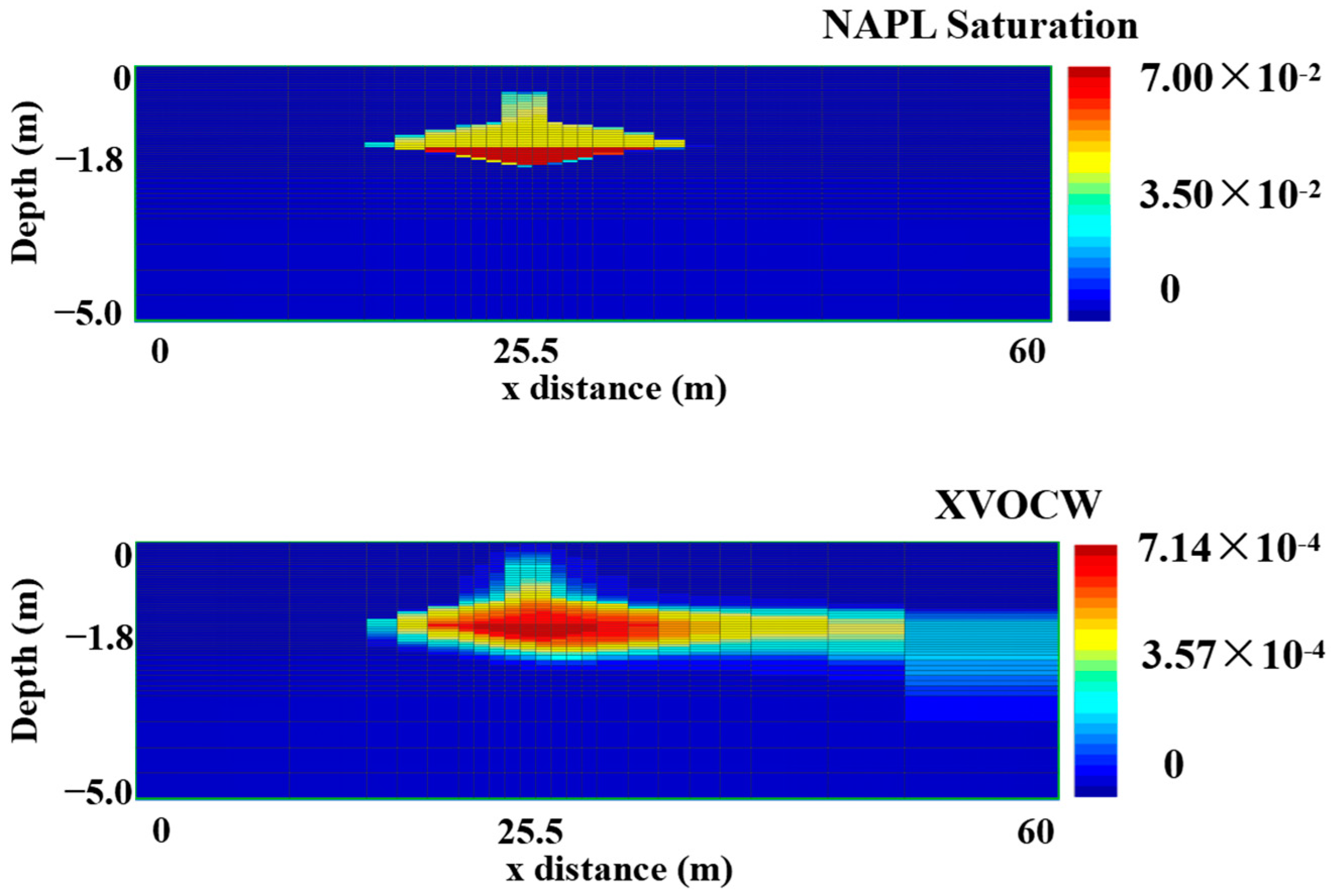
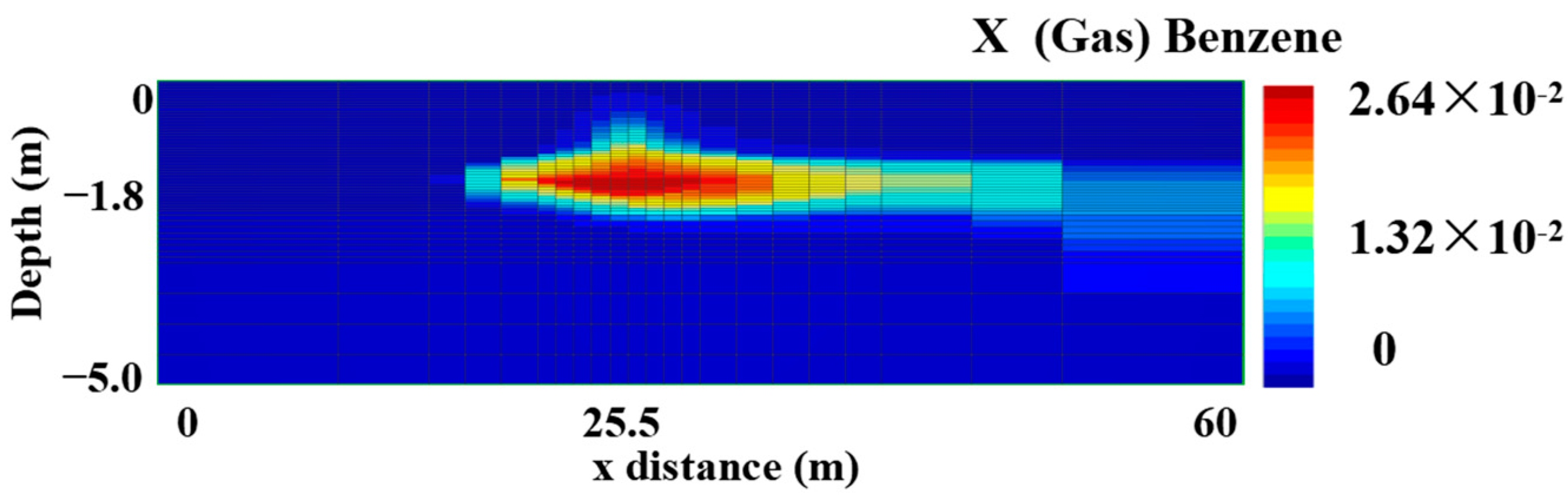
3.1. Modeling the Natural Spill State

The simulation was performed for 1.5 years under specified boundary conditions to achieve equilibrium between gravity and capillary pressure. The upper boundary was a fixed atmospheric boundary (P = 1.013 × 10⁵ Pa), and thermal, chemical, physical, and material exchanges with the atmosphere took place during the simulation. Hence, the effect of the upper boundary on the gas flow and the material balance was negligible in the simulation. Although these remained constant during the simulation, the left and right boundary cells were exposed to thermal, chemical, physical, and material exchanges with the external environment during the simulation to ensure material balance and allow groundwater flow.

Figure 2 shows the pressure distribution in the simulation area at equilibrium under gravity and capillary pressure. As shown, the pressure in the unsaturated zone was consistent with the atmospheric pressure, while the pressure in the saturated zone increased (up to 1.34 × 10⁵ Pa) with increasing depth. The initial GT in the model was at −1.8 m. After the stabilization of the model, the SVE of BTEX was executed for 12 months. After SVE at a constant GT for two months, the removal rate of each pollutant was 1 kg/d. Table S5 summarizes the physicochemical properties of different pollutants. The overall mass of BTEX was 1.65 × 10² kg and the mass fractions of benzene, toluene, ethylbenzene, and o-xylene were 17.25%, 24.23%, 28.98%, and 29.52%, respectively. As shown in Table S5, the solubilities and volatilities of benzene and toluene were significantly higher than those of ethylbenzene and o-xylene and benzene had the highest solubility and volatility.

Figure 3 illustrates the ratios of different components in the overall mass of leaked pollutants and masses of gaseous pollutants, aqueous pollutants, and pollutants in the NAPL phase. As observed, gaseous and aqueous pollutants followed the order of benzene > toluene > ethylbenzene > o-xylene. Additionally, ethylbenzene and o-xylene had similar fractions in the mass of pollutants in the NAPL phase, and their fractions exceeded those of the other two pollutants [43,44,45].

Figure 4 exhibits the NAPL saturation distribution of BTEX and the mass fraction distribution of dissolved BTEX (XVOCW). BTEX focused near the GT and a lenticular oil layer was generated due to low density (<ρ_water). In addition, BTEX will diffuse horizontally and penetrate through the GT under surface tension, capillary force, and buoyancy. BTEX were intercepted by soil pores, and BTEX in the NAPL phase were observed in soil pores during their vertical and horizontal migrations. The width and depth of the BTEX plume could be up to 40 m and 3 m, respectively. BTEX was exposed to dissolution and diffusion in groundwater. In simulations, the overall mass of BTEX could be 1.65 × 10² kg, which consists of 0.04%, 3.69%, and 96.27% of gaseous BTEX, aqueous BTEX, and BTEX in NAPL phases, respectively. Furthermore, saturation distributions of BTEX in the NAPL phase were proportional to mass fraction distributions of dissolved BTEX. The NAPL saturation could be up to 0.07, and BTEX with high saturation horizontally concentrated at the GT. The mass fraction of dissolved BTEX could be up to 7.14 × 10⁻⁴, and BTEX with high mass fractions concentrated vertically at the leaking point and horizontally at the GT. Both BTEX in the NAPL phase and dissolved BTEX diffused along the GT layer.

3.2. SVE System Design

3.2.1. Extraction Well Pressure

In SVE systems, the pressure in the extraction well is typically 0.90–0.95 atm. To determine the optimized pressure in the extraction well for the target site, 10-day SVE was executed at extraction well pressures of 0.90, 0.91, 0.92, 0.93, 0.94, and 0.95 atm, respectively. Figure S1 shows masses of residual BTEX at different extraction well pressures. As observed, the mass of residual BTEX was inversely proportional to the extraction well pressure. Therefore, 0.90 atm was used as the optimized extraction well pressure in this study.

3.2.2. Influencing Radius

The influencing radius (R_I), which is a key parameter in SVE, can be determined empirically or using steady-state pilot tests. Pressure drops in the extraction and monitoring wells can be determined using pilot tests, and pressure distributions in the stratum can be clarified using the calculation formula for a steady-state runoff with boundary conditions:

$$P_r^2-P_r^2=\left(P_{RI}^2-P_w^2\right)\frac{\ln \left(r/R_w\right)}{\ln \left(R_I/R_w\right)}$$

(1)

where P_r represents the pressure at a point whose distance from the gaseous extraction well is r (atm); P_w is the gaseous extraction well pressure (atm); P_RI represents the pressure at the tip of the influencing circle (atm); r represents the distance to the gaseous extraction well (m); R_I means the influencing radius (m); and R_w is the radius of the gaseous extraction well (m).

Pressure drops in both the extraction and monitoring wells were obtained using time-related simulations due to the absence of pilot tests. The one-year, single-well SVE at extraction well pressure = 0.90 atm showed that the pressure in the monitoring well (which is 5 m away from the extraction well) was 0.99 atm, and the diameter of the extraction well was 4 ft ≈ 0.1016 m. The location corresponding to the pressure drop was 1% saturation degree (0.10 atm), defined as R_I. Hence, P_RI = 1 − (0.10) (1%) = 0.999 atm. By substituting that into Equation (1), R_I can be calculated as 8 m.

3.2.3. Quantity of Extraction Wells

The quantity and locations of extraction wells were determined using the method that the influencing circles of all extraction wells (R_I = 8 m) can cover the whole simulation area [42]. Figure 5 shows the molar fraction distribution of benzene, which is the dominant component of gaseous pollutants. Three extraction wells were set at r = 22 m (W1), 37 m (W2), and 53 m (W3), respectively. BTEX with high mass fractions concentrated at leaking points near the GT, and the influencing radii of W1 and W2, which were close to leaking points, overlapped for 7%. Table S6 provides the locations of the three extraction wells.

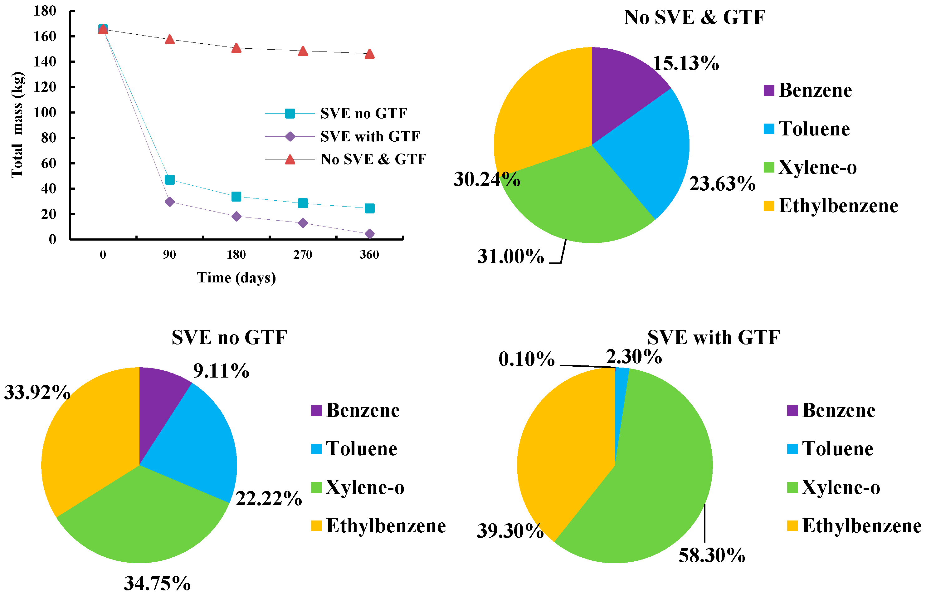
3.3. Removal Rates of BTEX

Figure 6 shows the changes in the overall mass of BTEX and mass fractions of different pollutants in all scenarios. In Scenarios 1, 2, and 3, the overall mass of BTEX decreased by 19.01, 140.92, and 161.05 kg, respectively; the removal rates of benzene, toluene, ethylbenzene, and o-xylene were 11.49%, 85.16%, and 97.33% (

Table 1. Removal rates of BTEX.

Scenarios		0 Day	90 Days	180 Days	270 Days	360 Days	Removal Rate (%) *
Total mass (kg)	SVE no GTF	165.48	47.07	33.86	28.55	24.55	85.16%
	SVE with GTF	165.48	29.77	18.25	13.06	4.42	97.33%
	No SVE & GTF	165.48	157.58	150.79	148.55	146.47	11.49%
Benzene mass (kg)	SVE no GTF	28.55	6.42	4.31	3.07	2.24	92.17%
	SVE with GTF	28.55	1.45	0.30	0.07	0.00	100.00%
	No SVE & GTF	28.55	25.75	23.35	22.72	22.15	22.42%
Toluene mass (kg)	SVE no GTF	40.12	10.35	7.89	6.50	5.46	86.40%
	SVE with GTF	40.12	5.97	3.16	1.82	0.11	99.74%
	No SVE & GTF	40.12	37.79	35.75	35.16	34.62	13.71%
Ethylbenzene mass (kg)	SVE no GTF	47.96	14.79	10.69	9.37	8.33	82.63%
	SVE with GTF	47.96	10.65	6.99	5.19	1.74	96.37%
	No SVE & GTF	47.96	46.52	45.28	44.78	44.30	7.63%
Xylene-o mass (kg)	SVE no GTF	48.85	15.51	10.98	9.60	8.53	82.53%
	SVE with GTF	48.85	11.70	7.80	5.98	2.58	94.72%
	No SVE & GTF	48.85	47.53	46.41	45.89	45.41	7.05%

Note: * Removal rate = (the mass of 360 days -the mass of 0 day)/the mass of 0 day.

and

Table 2. Removal rates of BTEX among gas, aqueous, and NAPL phases.

Scenarios		Days	Gas Phase (kg)	Aqueous Phase (kg)	NAPL Phase (kg)	Total Mass (kg)
No SVE and GTF	Benzene	0	0.0237	3.14	25.39	28.55
		360	0.0206	3.19	18.94	22.15
	Removal rate (%) *		13.18%	−1.71%	25.41%	22.42%
	Toluene	0	0.0169	1.26	38.84	40.12
		360	0.0203	1.40	33.19	34.62
	Removal rate (%) *		−20.13%	−11.26%	14.54%	13.71%
	Ethylbenzene	0	0.0117	0.45	47.50	47.96
		360	0.0181	0.54	43.74	44.30
	Removal rate (%) *		−54.34%	−19.61%	7.91%	7.63%
	Xylene-o	0	0.0094	0.55	48.30	48.85
		360	0.0146	0.65	44.74	45.41
	Removal rate (%) *		−55.23%	−19.40%	7.36%	7.05%
SVE no GTF	Benzene	0	0.0237	3.14	25.39	28.55
		360	0.0042	0.29	1.94	2.24
	Removal rate (%) *		82.41%	90.75%	92.35%	92.17%
	Toluene	0	0.0169	1.26	38.84	40.12
		360	0.0035	0.14	5.32	5.46
	Removal rate (%) *		79.41%	89.17%	86.31%	86.40%
	Ethylbenzene	0	0.0117	0.45	47.50	47.96
		360	0.0024	0.06	8.27	8.33
	Removal rate (%) *		79.25%	87.16%	82.59%	82.63%
	Xylene-o	0	0.0094	0.55	48.30	48.85
		360	0.0021	0.07	8.46	8.53
	Removal rate (%) *		78.01%	86.94%	82.48%	82.53%
SVE with GTF	Benzene	0	0.0237	3.14	25.39	28.55
		360	7.55 × 10−6	3.86 × 10−4	2.24 × 10−6	3.96 × 10−4
	Removal rate (%) *		99.97%	99.99%	99.99%	99.99%
	Toluene	0	0.0169	1.26	38.84	40.12
		360	0.0012	0.02	0.08	0.11
	Removal rate (%) *		92.88%	98.03%	99.79%	99.74%
	Ethylbenzene	0	0.0117	0.45	47.50	47.96
		360	0.0067	0.08	1.65	1.74
	Removal rate (%) *		42.53%	81.20%	96.53%	96.37%
	Xylene-o	0	0.0094	0.55	48.30	48.85
		360	0.0063	0.12	2.45	2.58
	Removal rate (%) *		32.65%	77.82%	94.92%	94.72%

Note: * Removal rate = (the mass of 360 days -the mass of 0 day)/the mass of 0 day.

), respectively. Furthermore, mass losses of BTEX in Scenarios 2 and 3 were significantly higher than that in Scenario 1. SVE exerts a significant effect on BTEX removal rates. This can be attributed to the negative pressure in the extraction well. Gaseous pollutants can be extracted within influencing circles of extraction wells in soil pores, due to the presence of this negative pressure, when these gases passed through the polluted area. As a result, both the concentration and mass of gaseous pollutants decreased, and aqueous pollutants and pollutants in the NAPL phase were subjected to volatilization due to the concentration gradient. In this way, the overall mass of pollutants decreased continuously. Additionally, the overall mass loss of BTEX in Scenario 3 was 12.17% higher than that in Scenario 2. The remediation performance of SVE in the presence of GTFs was superior to that in the absence of GFTs.

The mass fractions of benzene and toluene decreased, whereas the mass fractions of ethylbenzene and o-xylene increased. The mass loss of benzene exceeded that of the other three pollutants. The mass removal rates of benzene were 22.42%, 92.17%, and 99.99% in Scenarios 1, 2, and 3, respectively; the mass removal rates of toluene were 13.71%, 86.40%, and 99.74% in Scenarios 1, 2, and 3, respectively; the mass removal rates of ethylbenzene were 7.63%, 82.63%, and 96.37% in Scenarios 1, 2, and 3, respectively; and the mass removal rates of o-xylene were 7.05%, 82.53%, and 94.72% in Scenarios 1, 2, and 3, respectively. Indeed, the removal rates of all pollutants in the presence of SVE exceeded 80%, indicating the good applicability of SVE for the removal of BTEX from the target site. Furthermore, GTFs exerted a positive effect on the removal of BTEX from the target site. Additionally, the removal of BTEX from the target site was affected by both the solubility and volatility of each pollutant. The maximum mass loss of benzene can be attributed to its high solubility and volatility.

3.4. Transformation of BTEX among Gas, Aqueous, and NAPL Phases

Figure 7 displays variations in the masses of BTEX in gas, aqueous, and NAPL phases for the three scenarios. As observed, the overall mass of BTEX and the mass of BTEX in the NAPL phase decreased continuously in all scenarios, while the masses of gaseous and aqueous BTEX only decreased continuously in Scenarios 2 and 3. However, the mass loss of BTEX in the NAPL phase exceeded the overall mass loss of BTEX in Scenario 1, indicating that the masses of gaseous and aqueous BTEX increased. In Scenario 1, pollutants in the NAPL phase tend to transform into gas and aqueous phases. As shown in Figure 4, BTEX in the NAPL phase did not migrate beyond the left and right boundaries. In other words, the overall mass loss was mainly due to the mass loss of BTEX in the NAPL phase caused by their transformation into gas and aqueous phases and migration to the atmosphere via the upper boundary (in the gas phase). In Scenarios 2 and 3, SVE was the dominant contributor to the mass loss of BTEX.

Initially, the mass fractions of BTEX in gas, aqueous, and NAPL phases were 0.04%, 3.69%, and 96.27% (

Table 3. Mass of BTEX among gas, aqueous, and NAPL phases.

Scenario 1: No SVE and GTF
Days		Gas Phase (kg)	Aqueous Phase (kg)	NAPL Phase (kg)	Total Mass (kg)
0		0.07	6.10	159.31	165.48
90		0.42	6.24	150.93	157.58
180		0.08	5.87	144.84	150.79
270		0.03	6.43	142.08	148.55
360		0.08	6.55	139.85	146.47
Mass fractions (%) *	0 days	0.04%	3.69%	96.27%	/
	360 days	0.27%	3.96%	95.78%	/
Scenario 2: SVE No GTF
Days		Gas phase (kg)	Aqueous phase (kg)	NAPL phase (kg)	Total mass (kg)
0		0.07	6.10	159.31	165.48
90		0.03	0.89	46.15	47.07
180		0.02	0.74	33.09	33.86
270		0.01	0.68	27.85	28.55
360		0.01	0.64	23.90	24.55
Mass fractions (%) *	0 days	0.04%	3.69%	96.27%	/
	360 days	0.06%	1.89%	98.05%	/
Scenario 3: SVE with GTF
Days		Gas phase (kg)	Aqueous phase (kg)	NAPL phase (kg)	Total mass (kg)
0		0.07	6.10	159.31	165.48
90		0.06	0.96	28.75	29.77
180		0.02	0.27	17.96	18.25
270		0.01	0.20	12.85	13.06
360		0.01	0.23	4.18	4.42
Mass fractions (%) *	0 days	0.04%	3.69%	96.27%	/
	360 days	0.19%	3.23%	96.58%	/

Note: * Mass fractions of BTEX in gas, aqueous, and NAPL phases.

), respectively. In Scenario 1, the mass fractions of BTEX in gas, aqueous, and NAPL phases were 0.27%, 3.96%, and 95.78%, respectively. In Scenario 2, the mass fractions of BTEX in gas, aqueous, and NAPL phases were 0.06%, 1.89%, and 98.05%, respectively. In Scenario 3, the mass fractions of BTEX in gas, aqueous, and NAPL phases were 0.19%, 3.23%, and 96.58%, respectively. Additionally, the mass losses of gaseous and aqueous BTEX were consistent in Scenarios 2 and 3, while the mass loss of pollutants in the NAPL phase in Scenario 3 exceeded that in Scenario 2.

The mass fraction of aqueous BTEX exceeded that of BTEX in the NAPL phase. GTFs in Scenario 3 facilitated the volatilization and dissolution of pollutants in the NAPL phase. Figure 8 shows a longitudinal section of NAPL saturation at the leaking point in all scenarios. Indeed, the NAPL saturation of BTEX in Scenario 3 was lower than that in Scenario 2. GTFs not only stimulated the vertical migration of pollutants in the NAPL phase but also facilitated contact of pollutants in the NAPL phase with water, thus facilitating the dissolution of pollutants in the NAPL phase. Additionally, XVOCW in Scenario 3 was lower than in Scenario 2, while the vertical distribution of XVOCW in Scenario 3 was broader than that in Scenario 2.

3.5. Mass Loss of BTEX

As discussed in Section 3.4, SVE contributed significantly to the mass loss of BTEX in Scenarios 2 and 3, while the mass loss of BTEX in Scenario 3 exceeded that of Scenario 3. Figure 9 illustrates longitudinal gas flow (FLO (gas)) and flow of gaseous pollutants (FLO (gas) VOC) at the leaking points (where a negative value indicates an output). In Scenario 2, the gas flow remained constant from Day 90 to Day 360, while the flow of gaseous pollutants decreased as the overall mass of BTEX decreased; the removal rates of pollutants remained constant at the late stage. In Scenario 3, the gas flow varied with GT: from Day 1 to Day 90 and Day 270 to Day 360, the GT decreased and gas flow increased; from Day 90 to Day 270, the GT increased and gas flow decreased.

Additionally, the vertical flow and coverage of gas in Scenario 3 exceeded those in Scenario 2. As the GT decreased, gas in soil pores and the unsaturated zone expanded, resulting in increased gas flow. In Scenario 3, the flow of gaseous pollutants degraded as the overall mass of BTEX decreased, while the vertical coverage of the flow of gaseous pollutants exceeded that in Scenario 2. The gas flow and flow of gaseous pollutants in Scenario 3, as well as their coverages, exceeded those in Scenario 2 [46]. Hence, the removal rates of BTEX in Scenario 3 exceeded those in Scenario 2. As the GT decreased, the gas flow and flow of gaseous pollutants, as well as their coverages, increased significantly. As a result, the extraction of gaseous pollutants from underground media using extraction wells was accelerated.

4. Conclusions

The migration and transformation of BTEX in three scenarios were effectively simulated by simplifying a riverside petrochemical site using the TMVOC model (without considering river intrusions). Simulations were validated based on the GT depth at the monitoring well. In this study, the removal rates of BTEX in Scenarios 1, 2, and 3 were 11.49%, 85.16%, and 97.33%, respectively, indicating that SVE can effectively remove BTEX. In all scenarios, the removal rates followed the order of benzene > toluene > ethylbenzene > o-xylene. Additionally, removal rates of BTEX were maximized in Scenario 3, which were 99.99%, 99.74%, 96.37%, and 94.72%, respectively.

An in-depth understanding of BTEX transformation in gas–aqueous–NAPL phases was provided in three scenarios with the simulation of TMVOC. The NAPL phase mass of the three scenarios lost 19.46 kg, 135.41 kg, and 155.13 kg, respectively. The main mass loss was the NAPL phase, which was significantly larger than the gas and aqueous phase. The NAPL phase is transformed into gas and aqueous phases, which are then expelled via volatilization or groundwater runoff. In Scenarios 2 and 3, the mass losses were mainly contributed by the SVE of gaseous pollutants, which facilitates the transformation of aqueous pollutants and pollutants in NAPL phases to gaseous pollutants. GTF facilitates contact of pollutants in the NAPL phase with water, thus facilitating the dissolution and volatilization of pollutants in the NAPL phase.

The simulation results for BTEX with SVE under different conditions were quantified, which provided optimization suggestions on SVE for the remediation of BTEX compounds in groundwater. In Scenario 3 with a decreasing GT, the gas flow and flow of gaseous pollutants, as well as their coverages, increased 25% significantly. As a result, the extraction of gaseous pollutants from underground media using extraction wells was accelerated. Therefore, it can be concluded that increased flows in extraction wells, when the GT decreases, can improve VOC removal rates.

References

1. Cavelan, A.; Colfier, F.; Colombano, S.; Davarzani, H.; Deparis, J.; Faure, P. A critical review of the influence of groundwater level fluctuations and temperature on LNAPL contaminations in the context of climate change. Sci. Total Environ. 2022, 806, 150412. [Google Scholar] [CrossRef] [PubMed]
2. Onna, C.; Olaobaju, E.A.; Amro, M.M. Experimental and numerical assessment of Light NonAqueous Phase Liquid (LNAPL) subsurface migration behavior in the vicinity of groundwater table. Environ. Technol. Innov. 2021, 23, 101573. [Google Scholar] [CrossRef]
3. Zhao, B.; Peng, T.; Hou, R.; Huang, Y.; Zong, W.; Jin, Y.; O’Connor, D.; Sahu, S.; Zhang, H. Manganese stabilization in mine tailings by MgO-loaded rice husk biochar: Performance and mechanisms. Chemosphere 2022, 308, 136292. [Google Scholar] [CrossRef] [PubMed]
4. Zhang, H.; Li, A.; Wei, Y.; Miao, Q.; Xu, W.; Zhao, B.; Guo, Y.; Sheng, Y.; Yang, Y. Development of a new methodology for multifaceted assessment, analysis, and characterization of soil contamination. J. Hazard. Mater. 2022, 438, 129542. [Google Scholar] [CrossRef]
5. Gribovszki, Z.; Szilágyi, J.; Kalicz, P. Diurnal fluctuations in shallow groundwater levels and stream flow rates and their interpretation—A review. J. Hydrol. 2010, 385, 371–383. [Google Scholar] [CrossRef] [Green Version]
6. Zuo, R.; Zheng, S.; Liu, X.; Wu, G.; Wang, S.; Wang, J.; Liu, J.; Huang, C.; Zhai, Y. Groundwater table fluctuation: A driving force affecting nitrogen transformation in nitrate-contaminated groundwater. J. Hydrol. 2023, 621, 129606. [Google Scholar] [CrossRef]
7. Wei, Y.; Xu, X.; Zhao, L.; Cao, X. Numerical modeling investigations of colloid facilitated chromium migration considering variable-density flow during the coastal groundwater table fluctuation. J. Hazard. Mater. 2023, 443 Pt B, 130282. [Google Scholar] [CrossRef]
8. Yang, M.; Zheng, Y.; Xu, X.; Liu, H.; Xin, P. Groundwater table fluctuations in a coastal unconfined aquifer with depth-varying hydraulic properties. J. Hydrol. 2022, 606, 127407. [Google Scholar] [CrossRef]
9. Wei, Y.; Xu, X.; Zhao, L.; Chen, X.; Qiu, H.; Gao, B.; Cao, X. Migration and transformation of chromium in unsaturated soil during groundwater table fluctuations induced by rainfall. J. Hazard. Mater. 2021, 416, 126229. [Google Scholar] [CrossRef]
10. Mainhagu, J.; Morrison, C.; Brusseau, M.L. Using vapor phase tomography to measure the spatial distribution of vapor concentrations and flux for vadose-zone VOC sources. J. Contam. Hydrol. 2015, 177–178, 54–63. [Google Scholar] [CrossRef] [Green Version]
11. US Environmental Protection Agency. Superfund Remedy Report Thirteenth Edition (EPA-542-R-10-004); Office of Solid Waste and Emergency Response: Washington, DC, USA, 2010.
12. Brusseau, M.L.; Mainhagu, J.; Morrison, C.; Carroll, K.C. The vapor-phase multi-stage CMD test for characterizing contaminant mass discharge associated with VOC sources in the vadose zone: Application to three sites in different lifecycle stages of SVE operations. J. Contam. Hydrol. 2015, 179, 55–64. [Google Scholar] [CrossRef] [Green Version]
13. You, K.; Zhan, H. Can atmospheric pressure and water table fluctuations be neglected in soil vapor extraction. Adv. Water Res. 2012, 35, 41–54. [Google Scholar] [CrossRef]
14. Yang, Y.; Li, J.; Lv, N.; Wang, H.; Zhang, H. Multiphase migration and transformation of BTEX on groundwater table fluctuation in riparian petrochemical sites. Environ. Sci. Pollut. Res. 2023, 30, 55756–55767. [Google Scholar] [CrossRef] [PubMed]
15. Chen, X.; Sheng, Y.; Wang, G.; Guo, L.; Zhang, H.; Zhang, F.; Yang, T.; Huang, D.; Han, X.; Zhou, L. Microbial compositional and functional traits of BTEX and salinity co-contaminated shallow groundwater by produced water. Water Res. 2022, 215, 118277. [Google Scholar] [CrossRef] [PubMed]
16. Mckenzie, E.R.; Siegrist, R.L.; Mccray, J.E.; Higgins, C. The influence of a non-aqueous phase liquid (NAPL) and chemical oxidant application on perfluoroalkyl acid (PFAA) fate and transport. Water Res. 2016, 92, 199–207. [Google Scholar] [CrossRef]
17. Joun, W.T.; Lee, S.S.; Koh, Y.E.; Lee, K. Impact of Water Table Fluctuations on the Concentration of Borehole Gas from NAPL Sources in the Vadose Zone. Vadose Zone J. 2016, 15, vzj2015-09. [Google Scholar] [CrossRef]
18. Xu, J.; Zheng, L.; Yan, Z.; Huang, Y.; Feng, C.; Li, L.; Ling, J. Effective extrapolation models for ecotoxicity of benzene, toluene, ethylbenzene, and xylene (BTEX). Chemosphere 2020, 240, 124906. [Google Scholar] [CrossRef]
19. Yang, Q.; Li, Y.; Zhou, J.; Xie, X.; Su, Y.; Gu, Q.; Kamon, M. Modelling of benzene distribution in the subsurface of an abandoned gas plant site after a long term of groundwater table fluctuation. Hydrol. Proc. 2013, 27, 3217–3226. [Google Scholar] [CrossRef]
20. Rivett, M.O.; Wealthall, G.P.; Dearden, R.A.; McAlary, T.A. Review of unsaturated-zone transport and attenuation of volatile organic compound (VOC) plumes leached from shallow source zones. J. Contam. Hydrol. 2011, 123, 130–156. [Google Scholar] [CrossRef]
21. Zhang, Q.; Wang, G.; Sugiura, N.; Utsumi, M.; Zhang, Z.; Yang, Y. Distribution of petroleum hydrocarbons in soils and the underlying unsaturated subsurface at an abandoned petrochemical site, North China. Hydrol. Proc. 2013, 28, 2185–2191. [Google Scholar] [CrossRef]
22. Teramoto, E.H.; Chang, H.K. Field data and numerical simulation of btex concentration trends under water table fluctuations: Example of a jet fuel-contaminated site in Brazil. J. Contam. Hydrol. 2017, 198, 37–47. [Google Scholar] [CrossRef] [Green Version]
23. Ugwoha, E.; Andresen, J.M. Sorption and phase distribution of ethanol and butanol blended gasoline vapours in the vadose zone after release. J. Environ. Sci. 2014, 26, 608–616. [Google Scholar] [CrossRef] [PubMed]
24. Lari, K.S.; Johnston, C.D.; Davis, G.B. Gasoline Multiphase and Multicomponent Partitioning in the Vadose Zone: Dynamics and Risk Longevity. Vadose Zone J. 2016, 15, vzj2015.07.0100. [Google Scholar] [CrossRef]
25. Moshkovich, E.; Ronen, Z.; Gelman, F.; Dahan, O. In Situ Bioremediation of a Gasoline-Contaminated Vadose Zone: Implications from Direct Observations. Vadose Zone J. 2018, 17, 1–11. [Google Scholar] [CrossRef] [Green Version]
26. Soares, A.A.; Albergaria, J.T.; Domingues, V.F.; Alvim-Ferraz, M.; Delerue-Matos, C. Remediation of soils combining soil vapor extraction and bioremediation: Benzene. Chemosphere 2010, 80, 823–828. [Google Scholar] [CrossRef] [Green Version]
27. Wang, Y.; Chen, L.; Yang, Y.; Li, J.; Tang, J.; Bai, S.; Feng, Y. Numerical Simulation of BTEX Migration in Groundwater Table Fluctuation Zone Based on TMVOC. Res. Environ. Sci. 2020, 33, 634–642. [Google Scholar]
28. Zheng, Q.-T.; Yang, C.-B.-X.; Feng, S.-J.; Wu, S.-J.; Zhang, X.-L. Influence mechanism of thermally enhanced phase change on heat transfer and soil vapour extraction. J. Contam. Hydrol. 2023, 257, 104202. [Google Scholar] [CrossRef]
29. Liang, C.; Yang, S.-Y. Foam flushing with soil vapor extraction for enhanced treatment of diesel contaminated soils in a one-dimensional column. Chemosphere 2021, 285, 131471. [Google Scholar] [CrossRef]
30. Sun, P.; Hua, Y.; Zhao, J.; Wang, C.; Tan, Q.; Shen, G. Insights into the mechanism of hydrogen peroxide activation with biochar produced from anaerobically digested residues at different pyrolysis temperatures for the degradation of BTEXS. Sci. Total Environ. 2021, 788, 147718. [Google Scholar] [CrossRef]
31. Bian, Y.; Zhang, Y.; Zhou, Y.; Feng, X. BTEX in the environment: An update on sources, fate, distribution, pretreatment, analysis, and removal techniques. Chem. Eng. J. 2022, 435, 134825. [Google Scholar]
32. Peng, T.; Zhao, B.; O’Connor, D.; Jin, Y.; Lu, Z.; Guo, Y.; Liu, K.; Huang, Y.; Zong, W.; Jiang, J.; et al. Comprehensive assessment of soil and dust heavy metal(loid)s exposure scenarios at residential playgrounds in Beijing, China. Sci. Total Environ. 2023, 887, 164144. [Google Scholar] [CrossRef]
33. Nguyen, V.T.; Zhao, L.; Zytner, R.G. Three-dimensional numerical model for soil vapor extraction. J. Contam. Hydrol. 2013, 147, 82–95. [Google Scholar] [CrossRef] [Green Version]
34. Wang, B.; Zhang, Y.; Gao, C.; Du, X.; Qu, T. Developing novel persulfate pellets to remediate BTEXs-contaminated groundwater. J. Water Process Eng. 2023, 52, 103505. [Google Scholar] [CrossRef]
35. Huang, H.; Jiang, Y.; Zhao, J.; Li, S.; Schulz, S.; Deng, L. BTEX biodegradation is linked to bacterial community assembly patterns in contaminated groundwater ecosystem. J. Hazard. Mater. 2021, 419, 126205. [Google Scholar] [CrossRef] [PubMed]
36. Perina, T. General well function for soil vapor extraction. Adv. Water Res. 2014, 66, 1–7. [Google Scholar] [CrossRef]
37. Suk, H.; Zheng, K.-W.; Liao, Z.-Y.; Liang, C.-P.; Wang, S.-W.; Chen, J.-S. A new analytical model for transport of multiple contaminants considering remediation of both NAPL source and downgradient contaminant plume in groundwater. Adv. Water Resour. 2022, 167, 104290. [Google Scholar] [CrossRef]
38. Battistelli, A. Modeling Multiphase Organic Spills in Coastal Sites with TMVOC V.2.0. Vadose Zone J. 2008, 7, 316–324. [Google Scholar] [CrossRef]
39. Guo, Y.; Wen, Z.; Zhang, C.; Jakada, H. Contamination characteristics of chlorinated hydrocarbons in a fractured karst aquifer using TMVOC and hydro-chemical techniques. Sci. Total Environ. 2021, 794, 148717. [Google Scholar] [CrossRef]
40. Vanantwerp, D.J.; Falta, R.W.; Gierke, J.S. Numerical Simulation of Field-Scale Contaminant Mass Transfer during Air Sparging. Vadose Zone J. 2008, 7, 294–304. [Google Scholar] [CrossRef]
41. Lekmine, G.; Lari, K.S.; Johnston, C.D.; Bastow, T.P.; Rayner, J.L.; Davis, G.B. Evaluating the reliability of equilibrium dissolution assumption from residual gasoline in contact with water saturated sands. J. Contam. Hydrol. 2017, 196, 30–42. [Google Scholar] [CrossRef]
42. Yang, Y.; Li, J.; Xi, B.; Wang, Y.; Tang, J.; Wang, Y.; Zhao, C. Modeling BTEX migration with soil vapor extraction remediation under low-temperature conditions. J. Environ. Manag. 2017, 203, 114–122. [Google Scholar] [CrossRef]
43. You, K.; Zhan, H.; Li, J. A new solution and data analysis for gas flow to a barometric pumping well. Adv. Water Res. 2010, 33, 1444–1455. [Google Scholar] [CrossRef]
44. Schumacher, B.A.; Minnich, M.M. Extreme Short-Range Variability in VOC-Contaminated Soils. Environ. Sci. Technol. 2000, 34, 3611–3616. [Google Scholar] [CrossRef]
45. Davidson, C.J.; Svenson, D.W.; Hannigan, J.H.; Perrine, S.A.; Bowen, S.E. A novel preclinical model of environment-like combined benzene, toluene, ethylbenzene, and xylenes (BTEX) exposure: Behavioral and neurochemical findings. Neurotoxicol. Teratol. 2022, 91, 107076. [Google Scholar] [PubMed]
46. Man, J.; Zhou, Q.; Wang, G.; Yao, Y. Modeling and evaluation of NAPL-impacted soil vapor intrusion facilitated by vadose zone breathing. J. Hydrol. 2022, 615 Pt A, 128683. [Google Scholar] [CrossRef]
Figure 1. Location of the site (top) and conceptual model.
Water 15 02477 g001
Figure 2. Pressure distribution after natural modeling.
Water 15 02477 g002
Figure 3. Mass fractions of BTEX in gas, aqueous, and NAPL phases.
Water 15 02477 g003
Figure 4. Saturation distribution of BTEX in the NAPL phase (top) and mass fraction distribution of dissolved BTEX (bottom).
Water 15 02477 g004
Figure 5. Mole fraction distribution of benzene in the gas phase.
Water 15 02477 g005
Figure 6. Mass loss of BTEX and percentage of each contaminant at the end of each case.
Water 15 02477 g006
Figure 7. Trends in BTEX masses and mass loss in gas–aqueous–NAPL phases for each case.
Water 15 02477 g007
Figure 8. Vertical distributions of NAPL saturation and XVOCW at the leaking point.
Water 15 02477 g008
Figure 9. Vertical profiles of FLO (gas) and FLO (gas) VOC at the center of the contamination source.
Water 15 02477 g009