Article

Advanced Machine Learning Techniques to Improve Hydrological Prediction: A Comparative Analysis of Streamflow Prediction Models

1
Department of Civil Engineering, Dr. Vishwanath Karad MIT World Peace University, Pune 411038, Maharashtra, India
2
Department of Thermal Engineering and Thermal Engines, Samara National Research University, Moskovskoye Shosse, 34, Samara 443086, Russia
3
Department of Civil Engineering, Dr. S. & S. S. Ghandhy Government Engineering College, Surat 395001, Gujarat, India
4
National Research Council of Italy, Institute for Agricultural and Forest Systems in Mediterranean (CNR-ISAFOM), 87036 Cosenza, Italy
*
Authors to whom correspondence should be addressed.
Water 2023, 15(14), 2572; https://doi.org/10.3390/w15142572
Submission received: 9 June 2023 / Revised: 6 July 2023 / Accepted: 12 July 2023 / Published: 13 July 2023
(This article belongs to the Special Issue Impacts of Climate Change on Hydrology and Water Resources)

Abstract

:
The management of water resources depends heavily on hydrological prediction, and advances in machine learning (ML) present prospects for improving predictive modelling capabilities. This study investigates the use of a variety of widely used machine learning algorithms, such as CatBoost, ElasticNet, k-Nearest Neighbors (KNN), Lasso, Light Gradient Boosting Machine Regressor (LGBM), Linear Regression (LR), Multilayer Perceptron (MLP), Random Forest (RF), Ridge, Stochastic Gradient Descent (SGD), and the Extreme Gradient Boosting Regression Model (XGBoost), to predict the river inflow of the Garudeshwar watershed, a key element in planning for flood control and water supply. The substantial engineering feature used in the study, which incorporates temporal lag and contextual data based on Indian seasons, leads it distinctiveness. The study concludes that the CatBoost method demonstrated remarkable performance across various metrics, including Mean Absolute Error (MAE), Root Mean Square Error (RMSE), and R-squared (R2) values, for both training and testing datasets. This was accomplished by an in-depth investigation and model comparison. In contrast to CatBoost, XGBoost and LGBM demonstrated a higher percentage of data points with prediction errors exceeding 35% for moderate inflow numbers above 10,000. CatBoost established itself as a reliable method for hydrological time-series modelling, easily managing both categorical and continuous variables, and thereby greatly enhancing prediction accuracy. The results of this study highlight the value and promise of widely used machine learning algorithms in hydrology and offer valuable insights for academics and industry professionals.

1. Introduction

Accurate prediction of daily river inflow is essential for effective water resource management [1]. Inflow predictions play a crucial role in decision-making for water managers and policymakers, influencing water allocation, reservoir operations, flood control measures, and drought mitigation strategies [2]. Accurate predictions enable optimized utilization of water resources by providing insights into availability and distribution. Reservoir operations rely on accurate inflow predictions to make informed decisions on water release and storage, considering downstream demands, flood control, and ecological factors [3,4]. During drought periods, precise inflow predictions help in proactive water supply management by implementing conservation measures, water use constraints, and exploring alternative sources [5]. Accurate inflow predictions support the development of robust drought management plans, ensuring sustainable water provision for communities and ecosystems. The use of accurate inflow predictions aids in mitigating risks, optimizing water storage, and facilitating efficient water resource management practices [6,7].
For estimating streamflow, a variety of techniques have been developed, many of which are physically based models that rely on experimental and statistical analysis [8]. Physically based streamflow forecasting models are based on certain hydrological hypotheses and require a large quantity of hydrological data for calibration [9]. The physical processes involved in the water cycle, such as interactions between rainfall and runoff and river routing, are described by these models. However, the accessibility and dependability of hydrological data could restrict the implementation of these models. Physically based models require accurate hydrological data as inputs, such as rainfall volume, intensity, and dispersion [10]. However, obtaining such data can be difficult, particularly in areas with weak monitoring infrastructure, costly data collection, or convoluted logistics. The calibration and validation processes of these models are hampered by the absence of precise and comprehensive hydrological data, which reduces the forecasting accuracy [11].
The advantage of physically based models is that they faithfully represent the hydrological system and the underlying physical processes. These models reveal information on the mechanics of runoff production and flow dynamics, making them helpful tools for understanding the behavior of watersheds [12]. They are particularly useful when a thorough understanding of the physical processes is necessary, like when analyzing how variations in land use or climatic conditions impact streamflow [13]. However, adopting physically based models has a number of disadvantages. In addition to the already noted data constraints, these models frequently need complicated parameterization, which can be difficult and imprecise. The calibration procedure entails changing model parameters to suit observed data, and the precision of the calibration is strongly influenced by the caliber and representativeness of the available data [14]. Unfortunately, this procedure is costly, involves a lot of work, takes a long time, and requires sample collection. As a result, scientists are becoming more and more interested in enhancing cutting-edge data-driven models for predicting streamflow. These models provide a viable alternative, since they need fewer data and are affordable.
Data-driven models have certain benefits over physically based models. Without using explicit physical equations, these models may discover patterns and connections directly from the available data [15]. Since they can handle a variety of input variables and capture nonlinear interactions, data-driven models are frequently more versatile and flexible [16]. Additionally, they have benefits for streamflow forecasting in data-scarce places, since they can make reasonably accurate forecasts even with limited hydrological data [17]. Data-driven models do, however, have certain drawbacks. They lack the ability to represent the underlying physical processes explicitly, which may limit their interpretability and generalizability in certain cases [18]. Data-driven models are also sensitive to the quality and representativeness of the training data. Biases or outliers in the data can significantly affect the model’s performance, and it may be challenging to identify and address these issues without a good understanding of the underlying hydrological processes [19,20].
Streamflow predictions may be divided into short-term and long-term predictions, depending on the time period [21]. For flood control systems, hourly and daily forecasting, often known as short-term or real-time forecasting, is very valuable [22]. In the case of a flood, these projections allow for prompt action and decision making. Authorities can decide on evacuation, emergency response, and resource allocation in accordance with projections that are provided on an hourly or daily basis [23]. Real-time predictions assist in keeping an eye on flood-prone areas and sending out early warnings, therefore reducing the loss of life and property [24]. Long-term forecasting, however, covers the weekly, monthly, and yearly timescales [25]. It helps in managing irrigation systems, operating reservoirs, and producing electricity [26]. These projections are essential for controlling irrigation systems, maximizing the use of water for agriculture, and preserving ecological harmony. Furthermore, precise long-term projections aid in the planning of hydropower generation, permitting the best use of water resources for the development of renewable energy [27]. Streamflow forecasting has significantly advanced with the introduction of data-driven models. These models evaluate historical streamflow data and uncover patterns and correlations using computational methods like machine learning (ML) and artificial intelligence (AI) [28].
The potential for improving the precision and dependability of daily river inflow projections is enormous. With the aid of these methods, it is possible to evaluate sizable amounts of historical data, spot trends, and build intricate connections between meteorological factors, hydrological parameters, and river inflows [29]. ML models may learn and generalize from the patterns by being trained on previous data, which enables these models to produce precise forecasts for upcoming inflow circumstances [30]. The management of water resources will directly benefit from increasing the daily river inflow projections’ accuracy with ML. The ability to make educated decisions that assure the best possible use of water resources, reduce the effects of floods and droughts, and promote sustainable development is a key capability of water managers and policymakers. By utilizing ML approaches, it can improve the accuracy of inflow predictions and contribute to better and more efficient methods of managing water resources, which will eventually be advantageous to society, the environment, and the economy [31]. Artificial neural networks (ANNs), support vector machines (SVMs), Random Forests (RFs), gradient boosting machines (GBMs), deep learning (DL) [32], long short-term memory (LSTM) [33], Gaussian processes (GPs), and physics-informed ML [34,35] are a few ML techniques utilized in streamflow forecasting. To accurately anticipate streamflow, these techniques take into account temporal dependencies, manage nonlinear patterns, and capture complicated linkages. They provide a variety of methods for better water resource management and impact reduction from floods.

1.1. Literature Review

1.1.1. Traditional Methods for River Inflow Prediction

For predicting river inflows, traditional methods have been applied in the area of hydrology. Statistical or empirical models based on historical data and certain hydrological factors are frequently used in these strategies [36]. Even while these conventional approaches have proved useful for understanding river inflow patterns and guiding water resource management decisions, they may have shortcomings in terms of capturing complicated non-linear interactions and managing huge datasets with a variety of influencing elements [37]. The autoregressive integrated moving average (ARIMA) model is a typical classical approach [38]. The temporal patterns and trends in data on river inflows may be captured using ARIMA models, which are often used in time series analysis [39]. They take into account the moving average (MA) component for accounting for the impact of prior prediction errors, the integrated (I) component for addressing non-stationary factors, and the auto-regressive (AR) component for modeling the dependency on previous inflow values. For predicting river inflow, physical based models like the Soil and Water Assessment Tool (SWAT) are frequently used in hydrology [40]. These models use elements including rainfall, land cover, soil properties, and terrain to mimic the hydrological processes, based on physical principles [41]. SWAT and similar models estimate river inflows by using mathematical equations to simulate the movement of water through the terrain.
Traditional approaches may have problems capturing non-linear relationships and managing large, complex datasets, even though they have been effective for hydrological forecasting. Since they typically rely on assumptions and simplifications of the underlying mechanics, their accuracy may occasionally be constrained [42]. Additionally, traditional methods with high labor and computational costs are less suitable for real-time forecasting applications. To manage these restrictions, researchers have adopted ML techniques, which provide more adaptability and flexibility in collecting complex patterns and processing enormous datasets. By automatically discovering patterns and correlations from data, ML techniques like ANN, SVM, and RF have shown promise in enhancing the accuracy and resilience of river inflow estimates.

1.1.2. Machine Learning Approaches for River Inflow Prediction

In recent years, there has been a lot of interest in the ability of ML algorithms to manage enormous datasets and capture intricate relationships in hydrological systems. These methods provide a data-driven approach to hydrological modeling, allowing for the creation of prediction models that are more precise [43,44]. Different ML techniques, including ANN, SVM, and decision trees, have been used in the context of river flow prediction to improve forecasting abilities [45,46]. Popular ML models for hydrological modeling include ANNs. ANNs are capable of capturing non-linear correlations between the goal variable of the river flow and the input variables of precipitation, temperature, and soil moisture [47]. They can generalize from prior data patterns to produce forecasts for upcoming timespans. Another ML method for predicting river flow is SVM. Finding the ideal decision boundary that divides several classes or forecasts river flow values based on input data is the goal of SVM algorithms. SVM models are efficient at capturing complicated correlations in hydrological processes and can handle high-dimensional data [48,49,50].
River flow prediction has also used decision trees and their ensemble approaches, including Random Forests (RFs). These algorithms create decision trees based on past data and employ them to anticipate future events. In order to increase forecast resilience and accuracy, RF merges numerous decision trees. It has been applied to streamflow forecasting to better capture interactions between different hydrological factors [51,52]. In streamflow forecasting, gradient boosting machines (GBMs) like the extreme gradient boosting regression model (XGBoost) [53] and LGBM [54] have grown in popularity. They focus on samples with large prediction errors and repeatedly incorporate weak models to produce a strong predictive model. GBMs are renowned for their capacity to handle missing data and complicated connections.
A special kind of recurrent neural network (RNN) called long short-term memory (LSTM) is made for sequential data. For short-term forecasting applications in particular, LSTMs have proved effective in capturing temporal relationships in streamflow data and producing precise forecasts [55,56]. Probabilistic models known as Gaussian processes (GPs) are capable of capturing errors in forecasts of streamflow. They have been applied to streamflow forecasting to offer not just point predictions but also prediction intervals that show the forecasts’ level of uncertainty [57]. Hybrid models mix several machine learning (ML) methods or incorporate ML with physical models [58]. For instance, data assimilation methods may be applied to merge physically based models with ML methods to increase prediction accuracy or incorporate actual streamflow data into ML models. To enhance model performance, [59] created hybrid particle swarm optimization (PSO) and the group method of data handling for short-term prediction of daily streamflow, [60] developed ML-based grey wolf optimization for the short-term prediction of streamflows, [61] used hybrid LSTM-PSO for the streamflow forecast, [62] combined different ML methods for daily streamflow simulation, and [63] used an LSTM-based DL model for streamflow forecasting using Kalman filtering.
For predicting river flow, ML techniques provide a number of benefits. They have the ability to manage non-linear relationships and adjust to shifting hydrological circumstances. A more thorough investigation of the hydrological processes is possible because of ML models’ ability to handle huge datasets with many impacting elements. Additionally, ML methods may combine several data sources, such as meteorological data, remote sensing data, and historical streamflow records, to increase forecast accuracy. But it is crucial to remember that ML models have their limits as well. For efficient model building, they need a large volume of high-quality training data. To make sure the models reflect pertinent hydrological processes, care must be taken in the selection of acceptable input variables and feature engineering. Additionally, if the training dataset is too short or the model complexity is not adequately managed, ML models may experience overfitting. A variety of machine learning methods, such as CatBoost, ElasticNet, k-Nearest Neighbors (KNN), Lasso, light gradient-boosting machine regressor (LGBM), Linear Regression (LR), multilayer perceptron (MLP), Random Forest (RF), Ridge, stochastic gradient descent (SGD), and the extreme gradient-boosting regression model (XGBoost), have been used to create models for predicting river inflow in the article. The most efficient method for forecasting river inflow has been determined after the compared results of their investigations into the efficacy of each methodology.
This research makes several contributions that highlight its novelty:
  • Comparative Evaluation: the study provides a comprehensive comparative evaluation of multiple machine learning models for predicting river inflow. While previous studies have explored individual models, this research systematically compares the performance of CatBoost, ElasticNet, KNN, Lasso, LGBM, Linear Regression, MLP, Random Forest, Ridge, SGD, and XGBoost. Such a comprehensive comparative analysis is novel in the context of river inflow prediction.
  • Time Series Analysis: the study specifically focuses on time series analysis for river inflow prediction. Time series data present unique challenges, due to temporal dependencies. By applying different machine learning techniques to this specific domain, the research contributes to the advancement of time series prediction methodologies in the context of water resource management.
  • Application to River Inflow Prediction: while machine learning models have been applied in various domains, their application to river inflow prediction is of significant importance for water resource management. Predicting river inflow accurately is crucial for making informed decisions regarding water allocation, flood management, and hydropower generation.
  • Performance Evaluation on Multiple Datasets: the study evaluates the performance of the models on multiple datasets, including training, validation, and testing data. This comprehensive evaluation provides a robust assessment of the models’ performance and their ability to generalize to unseen data, contributing to the understanding of their efficacy in real-world scenarios.

1.2. Objectives of the Study

The primary objective is to develop models for predicting river inflow using the different machine learning methods mentioned, including CatBoost, ElasticNet, k-Nearest Neighbors (KNN), Lasso, light gradient-boosting machine regressor (LGBM), Linear Regression (LR), multilayer perceptron (MLP), Random Forest (RF), Ridge, stochastic gradient descent (SGD), and the extreme gradient-boosting regression model (XGBoost). The models attempt to forecast river inflow based on relevant input characteristics.

2. Methodology and Methods

The steps involved in developing and analyzing a machine learning (ML) model for predicting daily river inflow are outlined. Several important parts of the procedure are included. First, data from credible sources are used to compile historical data on daily river inflow. To guarantee data quality, the obtained data go through preprocessing, which includes cleaning and addressing missing values. Then, using feature engineering approaches, pertinent characteristics are extracted, including seasonal and temporal trends. A piece of the dataset is used to construct and train the models, while a different subset is used to validate their performance and evaluate their correctness. Common evaluation metrics, such as mean squared error (MSE), mean absolute error (MAE), root mean squared error (RMSE), root mean square percentage error (RMSPE) and R-squared (R2), are used to quantify the model’s performance.
To learn more about the model’s predictive skills and the importance of various characteristics in predicting river input, the generated data are carefully studied. The model’s implications for managing water resources are examined, along with suggestions for more study and possible practical application. By following this methodology, the study aims to contribute to the development of a robust and accurate model for daily river inflow prediction, which can provide valuable insights for effective water resource management and decision-making processes. Figure 1 shows the flowchart of the methodology of the study.

2.1. CatBoostRegressor Algorithm

CatBoostRegressor is an ML technique that predicts continuous values using gradient-boosted decision trees. It is a relatively new algorithm [64]. CatBoostRegressor is known for its efficiency, precision, and capacity for handling categorical characteristics. In order for the CatBoostRegressor algorithm to function, a set of weak decision trees must first be built. A powerful model is then built by combining these trees. Gradient boosting is the method used to join the trees. Gradient boosting works by adding additional trees to the model that fix the mistakes created by the earlier trees. To predict continuous values, CatBoostRegressor applies the following formula, as shown in Equation (1):
y = f x = i = 1 n α i   h i ( x )
where the output function f x is a linear combination of the basis functions h i ( x ) , and coefficients α i define the weight of each basis function in the linear combination; y is the predicted value, x is the input features.
The gradient descent method is used to calculate the model coefficients. The loss function must be minimized in the CatBoost. The difference between the values that were predicted and the actual values is measured by the loss function. A number of regression problems may be solved with the potent ML method CatBoost. It works especially effectively for issues involving categorical characteristics.

2.2. k-Nearest Neighbors

The KNN algorithm is a non-parametric regression method used for predicting the target variable based on the average of the target values of its k nearest neighbors [65]. Here are the key steps:
  • Prepare the training data with input features and target values.
  • Determine the value of k, the number of nearest neighbors to consider.
  • Calculate the distance between the new data point and the training data points.
  • Select the k nearest neighbors, based on the distances.
  • Calculate the target values’ average among the k closest neighbors. Use the average value as the new data point’s estimated goal value.
In Equation (2), the target variable prediction formula is shown, where ( y ^ ) is the predicted target value, k is the number of nearest neighbors, and y i is the sum of the target values of the k nearest neighbors.
y ^ = 1 k y i
The k-Neighbors Regressor technique is useful for detecting local patterns, managing non-linear connections, and making the fewest assumptions possible regarding the distribution of the data. However, it can be computationally demanding, sensitive to the selection of k and distance metric, and may call for feature scaling or regularization methods.

2.3. Light Gradient-Boosting Machine Regressor (LGBM)

The effectiveness and adaptability of the LGBM gradient-boosting method are well recognized. It provides a number of features and enhancements to optimize the performance of gradient boosting on big datasets [66]. In the data preparation stage of the method, the training data are divided into input characteristics and target values for regression. Target values and metric characteristics are recommended. The learning rate, number of trees, maximum depth, and feature fraction are then initialized. The LGBM model’s behavior is governed by these variables, which can be changed to enhance performance. Making a series of decision trees is part of the model creation and training process. A gradient-based optimization approach that minimizes the loss function is used to construct each tree. The ensemble of trees is iteratively expanded, and the predictions of the model are modified in accordance with the gradients of the loss function. After the model has been trained, additional data points may be predicted by using it. The LGBM method uses a weighted sum to aggregate the forecasts from each tree in the ensemble. During the training phase, the weights are chosen depending on the gradients of the loss function. In LGBM, the target variable may be predicted using the following formula:
y ^ = α i   h i ( x )
where α i indicates the weight given to the i t h tree, y ^ predicts the target value, and h i ( x ) the prediction of the i t h tree for the input characteristics x . The LGBM can capture complex non-linear correlations between characteristics and the target variable, is quite effective, and can handle enormous datasets. The loss function is optimized via gradient-based optimization, which creates an ensemble of trees that collectively provide precise predictions.

2.4. Linear Regression (LR)

LR method that deals with a set of records having X and Y values. These values are utilized to learn a function that can predict Y for an unknown X . In regression, the aim is to find the value of Y , given that X Y is continuous. Here, Y is referred to as the criterion variable, and X is called the predictor variable. Different types of functions or models can be employed for regression, wherein a linear function is the simplest one [67]. In this case, X can be a single or multiple features that represent the problem.
Y = C 1 + C 2 × X
where, X = input training data, Y = predicted value of Y for a given X , C 1 = intercept, and C 2 = coefficient of X. Once the optimal values of C 1 and C 2 are determined, the best fit line can be obtained.

2.5. Multilayer Perceptron

The Multilayer Perceptron (MLP) is a sort of artificial neural network that is made up of several layers of linked nodes, or neurons [68]. Since it is a feed-forward neural network, data goes from the input layer to the hidden layers and finally to the output layer. Each neuron in the MLP conducts a weighted sum of its inputs, applies an activation function to the sum, and then transmits the outcome to the neurons in the next layer. The following is a description of the MLP:
(a)
Assign random weights to the connections between the neurons as part of the initialization process.
(b)
The input layer: Take in input data and send them to the top-most hidden layer.
(c)
Hidden layers: Each hidden layer neuron computes the weighted sum of its inputs using the current weights and then applies an activation function (such as a sigmoid) to the sum.
(d)
Output layer: The neurons in the output layer compute the same activation function and weighted sum as the neurons in the hidden layers.
(e)
The MLP’s final output is derived from the neurons in the output layer.
During the training phase, the MLP’s weights are modified using optimization methods like gradient descent. A loss function that calculates the difference between the output that was expected and the output that was actually produced must be minimized. In order to produce predictions or categorize data based on fresh input, the MLP must first understand the underlying patterns and relationships in the data.

2.6. Random Forest

Random Forest (RF) is a highly accurate and versatile regression model widely used in ML. It belongs to the ensemble learning category, where multiple decision trees are built during the training phase. Each tree predicts the mean value of the target variable [69]. The steps involved in the Random Forest algorithm are as follows:
  • Random Subset Selection: a random subset of data points is chosen from the training set. This subset typically contains a fraction of the total data points, denoted by ‘p’.
  • Construction of a Decision Tree: using the subset of data points that was chosen, a decision tree is built. This procedure is repeated using various subsets of the data for a total of ‘N’ trees.
  • Prediction Aggregation: each of the ‘N’ decision trees predicts the value of the target variable for a new data point. The outcomes of all the predictions from the trees are averaged to provide the final forecast.
When using environmental input factors to forecast rainfall data, Random Forest is highly effective. The technique uses the combined predictive capability of the trees to decide the resultant class by creating a large number of decision trees during training. It is known for its effectiveness in handling large datasets and can produce reliable results even when dealing with missing data.

2.7. Lasso

Lasso, also known as L1 regularization, is a linear regression model that adds a penalty term based on the L1 norm of the coefficients [70]. It is used to encourage sparsity in the coefficient values, effectively performing feature selection by driving some coefficients to exactly zero. The formula for Lasso regression can be represented as follows:
y = β 0 + β 1 x 1 + β 2 x 2 + + β p x p
In addition to the mean squared error (MSE) factor, the objective function of Lasso regression also contains a regularization term:
L a s s o   O b j e c t i v e   F u n c t i o n = MSE + α × L 1   N o r m
where y stands for the dependent variable, and the independent variables (input characteristics) are represented by x 1 , x 2 , …, and x p . The independent variables’ coefficients (parameters) are β 0 , β 1 , β 2 , …, β p . The L1 regularization’s strength is determined by the regularization parameter, which is α . It chooses the appropriate ratio between punishing the size of the coefficients (L1 norm) and fitting the training data (MSE term).
The objective function’s L1 norm term is calculated as the sum of the absolute values of the coefficients.
L 1   N o r m = | β 1 | + | β 2 | + + | β p |
Lasso regression searches for the best values of the coefficients to minimize the MSE term while maintaining the L1 norm term as minimal as possible by minimizing the goal function. Thus, certain coefficients may be reduced to absolute zero, thus removing the related characteristics from the model. Because of this characteristic, Lasso regression may be used to handle high-dimensional datasets and feature selection.

2.8. Ridge

Ridge regression is an ML method frequently applied to regression analysis in the context of supervised learning. Regression analysis frequently uses Ridge regression, commonly referred to as Tikhonov regularization, to address the multicollinearity and overfitting issues [71]. It is an extension of ordinary least squares (OLS) regression that modifies the loss function by including a punishment component. The Ridge regression formula is as follows:
m i n i m i z e = | | Y X β | | 2 + λ | | β | | 2
Here, the target variable is denoted by Y , the predictor variables are denoted by X , the coefficients are denoted by β , the regularization parameter is denoted by λ controlling how much shrinkage is done to the coefficients, and the Euclidean norm is denoted by | | β | | . Ridge regression seeks to reduce the sum of squared discrepancies between predicted and observed values ( Y X ) , while also penalizing the size of the coefficients ( | | β | | 2 ).

2.9. ElasticNet

ElasticNet is a linear regression model that combines the L1 (Lasso) and L2 (Ridge) regularization techniques [72]. It is designed to overcome some limitations of each individual method by introducing a penalty term that includes both L1 and L2 norms.
The formula for ElasticNet regression can be represented as follows:
y = β 0 + β 1 x 1 + β 2 x 2 + + β p x p
The objective function of ElasticNet includes two regularization terms, one for L1 regularization and another for L2 regularization, along with the mean squared error (MSE) term:
E l a s t i c N e t   O b j e c t i v e   F u n c t i o n = MSE + α [ λ 1 L 1   N o r m + λ 2 L 2   N o r m ]
where y represents the dependent variable (the target variable we want to predict). x 1 , x 2 , …, x p represent the independent variables (input features). β 0 , β 1 , β 2 , …, β p are the coefficients (parameters) of the independent variables. α is the mixing parameter that controls the balance between L1 and L2 regularization. It is between 0 and 1. Ridge regression is represented by a value of α = 0, Lasso regression is represented by a value of α = 1, and values in between represent a mixture of both. The regularization parameters λ 1 and λ 2 regulate the potency of L1 regularization and L2 regularization, respectively.

2.10. Stochastic Gradient Descent (SGD) Regressor

For regression challenges, ML algorithms like the Stochastic Gradient Descent (SGD) Regressor are utilized. It is a modification of the common Gradient Descent technique and is especially helpful in cases involving online and massively multi-user learning [73]. A randomly chosen subset of training data (mini-batches) is used to iteratively update the model’s parameters via the SGD Regressor. It is computationally effective and appropriate for big datasets, since it calculates the gradients of the loss function with respect to the model’s parameters using just the samples in the mini-batch. The SGD Regressor’s update formula for the model’s parameters is the same as the normal SGD’s:
θ _ n e w = θ _ o l d α J ( θ _ o l d ; x i , y i )
Here, the parameters of the model are represented by their current values ( θ _ o l d ), their updated values ( θ _ n e w ), the learning rate ( α ), the gradient of the loss function J with respect to the parameters evaluated at the current parameter values ( J ( θ _ o l d ; x i , y i ) ), and one training example ( x i , y i ). To achieve optimal convergence and performance, it is crucial to carefully choose the learning rate and mini-batch size. Additionally, the performance and stability of the algorithm may be enhanced by using strategies like learning rate schedules, momentum, and regularization. The SGD Regressor works well when faced with massive data volumes, high-dimensional feature spaces, and a steady stream of new data.

2.11. Extreme Gradient-Boosting Regression Model (XGBoost)

XGBoost is a regression model, a potent ensemble learning technique which uses gradient boosting and decision trees to make precise predictions. The XGBoost approach delivers a variety of performance-improving improvements while sharing a similar structure with other gradient-boosting regressors [74]. The XGBoost algorithm is described in the sections below:
  • Choosing the XGBoost model’s parameters, such as the learning rate, the number of trees, the maximum depth, and the feature fraction, is the step-one process. These variables can be altered to improve performance and regulate how the model behaves.
  • Create the model and train it: the XGBoost model is produced by the construction of several decision trees. A gradient-based optimization technique that minimizes the loss function is used to build each tree. The ensemble of trees is continuously expanded throughout the training phase, and predictions are updated in line with gradients in the loss function.
  • After model training, the model may be used to make predictions about fresh data points. The XGBoost method incorporates the predictions from each tree in the ensemble to obtain the final regression prediction. The particular method for combining the predictions is determined by the loss function that is used.

3. Model Training and Validation

Model training and validation are crucial steps in the machine learning process. In these stages, a dataset is modelled for training, and the model’s effectiveness is assessed on a separate dataset for validation. The goal is to develop a model that accurately predicts the future and generalizes well to new inputs. The model training and validation procedure is summarized as follows:
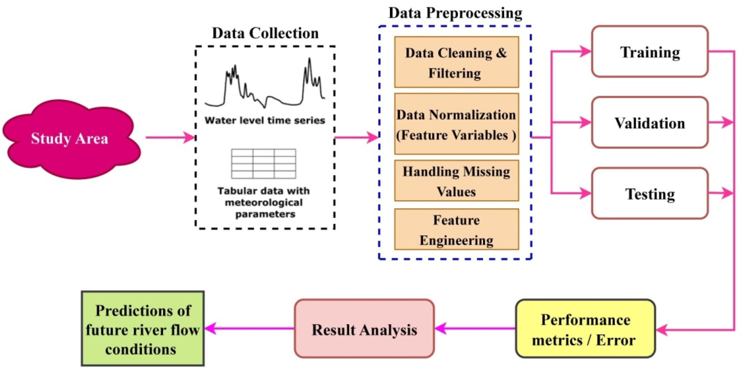
  • Data Split: a training set, a validation set, and a test set are each provided as separate datasets. The model is trained using the training set. The validation set is used to fine-tune the model and assess model performance throughout training, whereas the test set is used to measure the trained model’s final performance on unseen data.
  • Model Selection: select the most effective model architecture or machine learning technique for the particular job. The kind of data, the task (classification, regression, etc.), and the resources available are all factors in the model selection process.
  • Model Training: develop the selected model using the training dataset. During the training phase, the model parameters are frequently repeatedly improved in order to minimize a chosen loss or error function. In order to do this, training data are fed into the model, predictions are generated and compared to actual values, and model parameters are updated, depending on computed errors. This procedure continues until a convergence requirement is satisfied, after a certain number of epochs.
  • Model Evaluation: using the validation dataset, evaluate how well the trained model performed. The validation data is used to generate predictions, which are then compared to the actual results. There are several assessment measures employed, including mean squared error (MSE), mean absolute error (MAE), root mean square error (RMSE), root mean square percent error (RMSPE), and R-squared (R2) [75].
MSE = ( 1 / n ) [ ( y i y ^ i ) 2 ]
MAE = ( 1 / n ) | y i y ^ i |
RMSE = ( MSE ) = [ ( 1 / n ) [ ( y i y ^ i ) 2 ] ]
RMSPE = [ ( 1 / n ) [ ( ( y i y ^ i ) / y i ) 2 ] ]
R 2 = 1 ( [ ( y i y ^ i ) 2 ] / [ ( y i y ¯ ) 2 ] )
where the overall number of data points is n . The dependent variable’s actual (observed) value for the ith data point is represented by y i . The predicted value of the dependent variable for the ith data point is represented by y ^ i . Σ stands for the total sum, or the sum of the squared differences for each data point. The dependent variable’s mean is represented by the symbol y ¯ .
5.
Iterative Refinement: to enhance performance, modify the model architecture or data preparation stages based on the evaluation findings. Until a suitable performance is attained, this iterative procedure is continued.
6.
Final Assessment: after the model has been adjusted, its performance is evaluated using the test dataset, which simulates unseen data. This offers a neutral assessment of how well the model performs in realistic situations.
To guarantee accurate and trustworthy model training and assessment, it is crucial to remember that correct data preparation, including managing missing values, feature scaling, and controlling class imbalance, should be carried out during the training and validation process. These processes may be efficiently used to train, validate, and assess machine learning models, in order to create reliable and accurate prediction models.

4. Study Area, Data Collection and Preprocessing

4.1. Study Area

One of the largest rivers in central India, the Narmada River, passes through the states of Gujarat, Maharashtra, and Madhya Pradesh. The significance of it for ecology, history, and culture is widely known. Hindus adore the river’s waters and a variety of flora and animals call it home. In the Narmada River basin, the Garudeshwar gauging station is an important study location. The gauging station serves as a monitoring station for identifying and analyzing the river’s different hydrological properties. It is located close to the Gujarat town of Garudeshwar. The primary duty of the Garudeshwar gauging station is to gauge and track the water levels and flow rates of the Narmada River. The gauging station is equipped with instruments that gather data on a variety of elements, such as water level, discharge, and velocity. The research region around a gauging station is frequently defined by the gauging station’s measurement range of impact. This might alter, based on the objectives of the research specifically or the requirements of the water management authority. The research region may extend both upstream and downstream of the gauging station in order to completely comprehend the hydrological characteristics and dynamics of the river. Researchers, hydrologists, and managers of water resources routinely evaluate water availability, look into flood patterns, and make informed judgments regarding water distribution and management using the data collected from the gauging station and the study region. An overview of watershed areas and their placement on a map of India is shown in Figure 2.

4.2. Data Collection

Daily river inflow measurements in cubic meters per second were gathered from a river gauge station and utilized as the dataset for this investigation. The data, which span the years 1980 to 2019, were gathered from India’s Water Resources Information System (WRIS) for the time series analysis. A thorough record of the river’s inflow across time is provided by the dataset, allowing for examination of flow fluctuations and trends. Table 1 shows the descriptive statistics of the data.

4.3. Techniques for Preprocessing Data

Several preprocessing procedures can be used for the dataset from the Garudeshwar gauging station in order to guarantee the correctness and dependability of the data. To resolve errors, outliers, and missing numbers, the data must first be cleaned. This procedure comprises validation, cross-checking with trustworthy sources, and using statistical techniques and subject-matter expertise to spot and fix flaws and inconsistencies. Depending on their relevance, outliers can either be corrected or removed. The dataset’s integrity can be preserved by imputing missing values using techniques like mean imputation or interpolation. To improve the models’ ability to anticipate outcomes, feature engineering approaches can be used. This entails generating fresh features from preexisting variables. In the context of predicting river inflow, temporal characteristics can be derived from the date variable to identify trends in the data. Lagged features, which represent past inflow values, will also be generated to capture the influence of historical data on future predictions. The first seven days of 1980 (from 1 January to 7 January) are not taken into account to create lagged characteristics, so data here is available from 8 January 1980 to 31 December 2019. Also, no outliers and all peak data points have been taken into account, since there is no elimination of any data points.
An augmented Dickey–Fuller (ADF) statistic is used to check the stationarity or non- stationarity of the data. The ADF statistic is a test statistic used in time series analysis to determine the presence of a unit root in the data. The unit root refers to the presence of a stochastic trend that can cause non-stationarity in the series. If the series is found to be stationary, it implies that there is no significant linear trend present. In the given scenario, the ADF statistic has a value of −13.045793. This indicates a highly negative value, suggesting strong evidence against the presence of a unit root in the data. The p-value associated with the ADF statistic is reported as zero, which further supports the rejection of the null hypothesis of a unit root. To assess the significance level of the ADF statistic, critical values are considered. The critical values at 1%, 5%, and 10% significance levels are −3.431, −2.862, and −2.567, respectively. Since the ADF statistic value of −13.045793 is much lower (in absolute terms) than these critical values, it can conclude that the data is statistically significant and the result of the ADF statistic is shown in Figure 3. Therefore, based on the ADF statistic and its associated p-value, we can infer that the data under consideration are stationary. Stationary data implies that the statistical properties of the series, such as mean, variance, and autocorrelation, remain constant over time. This is an important characteristic for many time series analysis techniques and modeling approaches. It is significant to note that, depending on the location and features of the area under examination, the stationarity of river flow series might change. River flow series do occasionally display stationary qualities, despite the fact that seasonal patterns, trends, and other variables frequently cause river flow series to behave in a non-stationary manner. The particular location under consideration in this study may have unique characteristics that contribute to the observed stationarity. The stationarity of river flow series can be influenced by elements including the hydrological parameters of the river basin, climatic circumstances, land use patterns, and water management techniques. Furthermore, it is worth mentioning that even if the river flow series is stationary, it does not imply that the series is entirely predictable or that it lacks variability. The presence of other forms of variability, such as short-term fluctuations or irregular patterns, can still exist within a stationary series.
The original time series, trend, seasonality, and residual time series are displayed in Figure 4. With regard to the combined influences of trend, seasonality, and random fluctuations, the original data offer a thorough assessment of the real observations. The long-term, regular movement or direction of the river flow is represented by the trend flow component. It shows if the flow is increasing or decreasing over time. It can observe the general behavior of the river flow and spot any enduring alterations by focusing on the trend. In this instance, the trend flow indicates a declining pattern in the data of the river flow. This information is helpful in determining the general trend and making future plans for the management of water resources. Seasonality describes recurring, predictable fluctuations that take place at predetermined times. Seasonality in the context of river flow refers to regular patterns or fluctuations that take place over the course of a year. By examining the seasonality component, it locates any recurring patterns in the river flow data. In this case, the seasonality component varies by up to 4000 m3/s, demonstrating that the river flow displays significant patterns and changes throughout the year. Understanding seasonality can aid in forecasting future flow patterns and preparing for the demands placed on water resources throughout particular seasons. The residuals are the variations between the values that were seen and those that were anticipated by the trend and seasonality components. They stand for the arbitrary and unpredictable variations in river flow that neither trends nor seasonality can account for. Any remaining anomalies or out-of-the-ordinary events in the data can be understood by analyzing the residuals. The residuals allow us to determine the trend and seasonality components’ goodness of fit as well as any other variables affecting the river flow.

4.3.1. Creating Lagged Features

When working with time series data, the idea of “lagged features” is very pertinent. A value from a previous time period is a lagged characteristic from a time series. A lagged characteristic may be the river input from today, yesterday, or even a week ago if we are forecasting river inflow for tomorrow. These are known, correspondingly, as lag-1, lag-2, and lag-7 characteristics. Lagged features can be used to capture the temporal relationships present in the data. In other words, they offer a method of providing the model with information about previous values, which may be useful for forecasting future values. The lag order, which refers to the number of lagged data to include, is often established empirically, frequently by employing methods like autocorrelation plots or depending on domain knowledge. For this study, lagged features are implemented according to domain knowledge; daily data of a week are taken to predict next-day data.

4.3.2. Date Feature Engineering

The development of date features was a crucial preprocessing step in this work. In order to do this, more pertinent information must be extracted from the timestamp data. The study’s date characteristics included the weekday, the month, the Indian month, and the Indian season. These elements were included because they may have a large impact on river input. For instance, because of weather patterns, some months or seasons may see higher or lesser influx. Depending on the timestamp’s data format, different processes can be used to create various properties. Before these properties can be retrieved, the timestamp may need to be transformed from a string format into a datetime object. Once the features are finished, they may be used as any other model input.

4.3.3. One-Hot Encoding

One-hot encoding is the last preprocessing step. Categorical variables are handled using this technique. The categorical data must be translated into a format that can be used by these methods, since many machine learning algorithms cannot deal directly with categorical data. One-hot encoding is a typical method. Each distinct category of a categorical variable is represented as a binary vector in one-hot encoding. One-hot encoding would produce seven new features (one for each day of the week) if, for instance, the feature “day of the week” had seven categories (Monday, Tuesday, …, Sunday). If Monday were the day of the week, “Monday” would have a value of 1, while all other days would have a value of 0. If the day was Tuesday, the “Tuesday” feature would be set to 1, and all other day features would be set to 0, and so on. One-hot encoding completely eliminates any ordinal link between categories (i.e., it prevents the model from assuming that “Monday” is less than “Tuesday” just because we encode Monday as 1 and Tuesday as 2). This is advantageous when there is no ordinal link between the categories, as there is when talking about the days of the week, months, or seasons.

5. Model Preparation

In this investigation, the data were divided into training, validation, and test sets using a time series split. The temporal order of the observations is crucial in time series data; therefore, this approach of data splitting is very appropriate. The data are separated into time periods in a time series split. The earliest observations make up the training set, the sequence observations make up the validation set, and the latest observations make up the test set. This makes sure that each piece of data accurately depicts the chronological order of the actual occurrences. It is crucial to keep in mind that time series splits preserve the temporal dependencies and autocorrelation inherent in time series data, unlike random splits, which forbid the inclusion of any future data in the training set. On the basis of the patterns found in the historical data, the models were trained on the training set to predict the target variable. The models were then tested on the validation set, which contained data that were not utilized during training but temporally followed the training period. This stage allowed us to retain the data’s chronological integrity while monitoring the models’ performance on previously unknown data and making any required adjustments. The test set, which represented the most current data in the series, was used to evaluate the models. This provided a fair assessment of the models’ performance on brand-new, previously unobserved data, and an estimate of how well the models would perform when making predictions about upcoming real-world data. To retain the temporal structure of the data while assessing the predictive performance of our models by using a time series split, guaranteed that the models had the capacity to provide accurate future projections.

6. Results and Discussion

The prediction models in this research were meticulously evaluated, offering insightful information. Several machine learning models, including CatBoost, ElasticNet, KNN, Lasso, LGBM, Linear Regression, MLP, Random Forest, Ridge, SGD, and XGBoost, were assessed for their ability to predict river inflow. A range of error metrics and R-squared values were used to evaluate their performance.

6.1. Performance Metrics of Training Data

The performance indicators for several models based on training data are shown in Table 2. Each model is assessed using the metrics of MAE, MSE, RMSE, RMSPE, and R2. These metrics evaluate each model’s performance on the training data. Higher R2 values indicate a better fit of the model to the data, while lower MAE, MSE, RMSE, and RMSPE values denote superior performance. A comparison of the models in Table 2 reveals that CatBoost, XGBoost, and RF demonstrate improved prediction accuracy and model fit on the training data, due to their lower MAE, MSE, RMSE, RMSPE values and high R2. ElasticNet, KNN, Lasso, LR, MLP, Ridge, and SGD perform less effectively on the training data, having lower R2 and higher MAE, MSE, RMSE, RMSPE values. LGBM also performs well, exhibiting relatively low values across all the criteria. Models with the lowest errors (MAE, MSE, RMSE, RMSPE), highest R2, and best performance on the training data are CatBoost, XGBoost, and RF. These models fit the training data well, and have excellent predictive capabilities. It is crucial to note that a model’s performance on training data might not necessarily generalize to new data. Therefore, further assessment of the models’ overall performance using validation and test data is necessary to select the most suitable model for prediction tasks.

6.2. Performance Metrics of Validation Data

The performance characteristics of several models on the validation data are displayed in Table 3. For each model, the metrics are MAE, MSE, RMSE, RMSPE, and R2. After reviewing the performance of the models using validation data, the following conclusions can be drawn: LGBM, Lasso, MLP, and Ridge perform better on the validation data as a result of having comparatively lower values for MAE, MSE, RMSE, RMSPE, and higher R2. CatBoost, ElasticNet, LR, RF, SGD, and XGBoost also exhibit acceptable performance, with moderate metric values. KNN performs poorly on the validation data, with higher values for MAE, MSE, RMSE, RMSPE, and lower R2. LGBM, Lasso, MLP, and Ridge outperform the other models on the validation data. Their continuously decreased errors (MAE, MSE, RMSE, and RMSPE) and improved R2 on the validation set indicate increased model fit and prediction accuracy. However, it is crucial to consider the possibility that model performance on the validation data may not generalize to new data. Therefore, additional testing on other datasets, such as a different test set, is required.

6.3. Performance Metrics of Testing Data

The performance metrics of several models on the testing data are shown in Table 4. For each model, the metrics are MAE, MSE, RMSE, RMSPE, and R2. The following findings may be drawn from examining how well the models performed on the testing data: with lower MAE, MSE, RMSE, and RMSPE values and greater R2, LGBM, CatBoost, and MLP demonstrate improved performance on the test data. In addition to ElasticNet, Lasso, RF, Ridge, XGBoost, and others exhibit acceptable performance, with modest values for the metrics. The MAE, MSE, RMSE, RMSPE, and lower R2 values for KNN, LR, and SGD are comparatively greater, indicating poor performance on the testing data. LGBM, CatBoost, and MLP perform better on the testing data when compared to the other models. They routinely achieve reduced errors (MAE, MSE, RMSE, RMSPE), greater R2, and better model fit on the testing set, all of which indicate enhanced prediction accuracy.

6.4. Comparison of the Models

A comparison of the performance metrics across the three datasets (training, validation, and testing) was conducted to identify the best-performing model. The performance measures from each of the Table 2, Table 3 and Table 4 were observed.
  • Training Data: XGBoost has the highest R2 and the lowest MAE, MSE, RMSE, and RMSPE values, indicating the best performance on the training data. The time series prediction for XGBoost is shown in Figure 5, where predicted streamflow inflows are depicted alongside the actual data. The fundamental patterns and fluctuations in streamflow across the dataset are largely captured by the XGBoost model, as can be seen in this figure.
  • Validation Data: the LGBM model has the highest R2 and the lowest MAE, MSE, RMSE, and RMSPE values, demonstrating the best performance on the validation data. The time series prediction for LGBM against the actual data is shown in Figure 6.
  • Testing Data: LGBM has the highest R2 and the lowest MAE, MSE, and RMSE values, showing the best performance on the testing data.
The study’s findings provide strong evidence regarding the performance of different models on various datasets, with noticeable differences potentially attributable to overfitting or underfitting. In particular, the results suggest that XGBoost may have overfit the training dataset, resulting in less impressive performance on the test dataset, despite its excellent performance on the training data. Conversely, LGBM performed better on both the validation and testing datasets, suggesting its ability to generalize well to unseen data, although it showed poorer performance on the training set.
Among all, the CatBoost model demonstrated reliable generalization ability, showcased by its robust performance on the training and testing datasets. This suggests that CatBoost is capable of producing accurate predictions even for novel and untested data, as illustrated in Figure 7. However, based on these results, it remains challenging to definitively determine which model performed best in this study.
For clearer understanding, scatter plots (shown in Figure 8, Figure 9 and Figure 10) were generated to illustrate the correlation between the predicted and actual streamflow inflow for XGBoost, LGBM, and CatBoost. An examination of these figures reveals that most data points indicate an error of less than 10% for larger inflow values and less than 20% for moderate inflow levels. In contrast, both XGBoost and LGBM show a higher percentage of data points with errors exceeding 35% for moderate inflow levels above 10,000. Similarly, for CatBoost, inflow levels below 6000 exhibit a larger error rate, of about 35%. It is crucial to note that these lower inflow levels were not the primary focus of this investigation.
Additionally, as demonstrated in Figure 8, XGBoost not only exhibits evidence of overfitting to the training data but also generates inaccurate predictions for higher inflow values in the test data. This raises questions about the accuracy of XGBoost’s predictive capabilities under certain circumstances. However, as illustrated in Figure 9, LGBM struggles to accurately predict key factors related to higher inflow levels.
Taking all these factors into account, it can be confidently stated that the CatBoost model outperforms both XGBoost and LGBM in terms of robustness and reliability for inflow predictions. CatBoost is a particularly suitable choice for applications requiring accurate prediction of inflow quantities under specific circumstances. In summary, CatBoost emerges as the most reliable model and a viable option for predicting inflow.

6.5. Limitations of the Study

While the study has provided a comprehensive analysis of various machine learning models for river inflow prediction and identified the most reliable model, it is indeed essential to address the limitations of the study.
(a)
One limitation of our research is the reliance on a specific dataset from the Garudeshwar gauging station. The generalizability of the findings may be limited to this particular location, and may not directly apply to other river systems. Future studies should consider incorporating data from multiple gauging stations or rivers to validate the performance of the models across different regions.
(b)
Another limitation is the time frame of the dataset used in the study, which spans from 1980 to 2019. Although this provides a substantial historical perspective, it may not capture recent changes or evolving patterns in river inflow. Incorporating more up-to-date data would enhance the accuracy and relevance of the predictions.
(c)
Additionally, the study focused primarily on machine learning models and did not consider other factors that could influence river inflow, such as climate change, land use changes, or anthropogenic activities. Incorporating these factors into the modeling process may provide a more comprehensive understanding of the dynamics of river inflow.
(d)
Lastly, the performance of the models may be influenced by the quality and completeness of the data. Data quality issues, such as measurement errors, could impact the accuracy of the predictions. It is crucial for future research to address data preprocessing and quality control techniques to mitigate such limitations.

7. Conclusions

To effectively manage water resources, this study compared the efficacy of several machine learning models for predicting river inflow. Models including CatBoost, ElasticNet, KNN, Lasso, LGBM, LR, MLP, RF, Ridge, SGD, and XGBoost were all investigated. CatBoost consistently outperformed other models across all three datasets, displaying remarkable performance across various metrics. It achieved impressive R2 values on both the training and validation data, demonstrating a strong fit to the data and accurately capturing the variation in the target variable. Additionally, it performed well on the testing data, with relatively low MAE and RMSE values. LGBM also performed well across all three datasets, achieving competitive results for MAE, MSE, RMSE, and R2 on both the testing and validation data, and demonstrated reasonable MAE and RMSE on the testing data. LGBM, renowned for its effective gradient-boosting implementation and its ability to handle large datasets and capture intricate correlations, showcased these strengths in this study. Results from XGBoost were encouraging, especially when applied to the training and validation data. It achieved the lowest MAE, MSE, RMSE, and RMSPE values on the training set, demonstrating an excellent fit. It also displayed reasonably low MAE and RMSE on the validation data, indicating strong generalization. However, it performed somewhat worse than CatBoost and LGBM in terms of R2 scores on the testing data. Based on careful investigation and comparison from error plots, CatBoost was determined to have the best performance among the models. CatBoost performed optimally on the test data, demonstrating its ability to make accurate predictions on new, unseen data. Future studies should explore ensemble approaches, which combine the strengths of multiple models to enhance prediction accuracy. Incorporating domain knowledge and additional pertinent factors may also improve the performance of the models. To maintain the efficacy of these models in hydrological forecasting, continuous updating of the models with fresh data will be necessary.

Author Contributions

Conceptualization, V.K.; Software, V.K.; Validation, D.J.M.; Formal analysis, K.V.S. and D.J.M.; Investigation, N.K.; Writing—original draft, T.C.; Writing—review & editing, T.C. All authors have read and agreed to the published version of the manuscript.

Funding

This research received no external funding.

Data Availability Statement

The data presented in this study are available on request from the corresponding authors.

Conflicts of Interest

The authors declare no conflict of interest.

References

  1. El-Shafie, A.; Taha, M.R.; Noureldin, A. A neuro-fuzzy model for inflow forecasting of the Nile river at Aswan high dam. Water Resour. Manag. 2007, 21, 533–556. [Google Scholar] [CrossRef]
  2. Stakhiv, E.; Stewart, B. Needs for Climate Information in Support of Decision-Making in the Water Sector. Procedia Environ. Sci. 2010, 1, 102–119. [Google Scholar] [CrossRef] [Green Version]
  3. Kumar, V.; Yadav, S.M. Multi-objective reservoir operation of the Ukai reservoir system using an improved Jaya algorithm. Water Supply 2022, 22, 2287–2310. [Google Scholar] [CrossRef]
  4. Chabokpour, J.; Chaplot, B.; Dasineh, M.; Ghaderi, A.; Azamathulla, H.M. Functioning of the multilinear lag-cascade flood routing model as a means of transporting pollutants in the river. Water Supply 2020, 20, 2845–2857. [Google Scholar] [CrossRef]
  5. Venkataraman, K.; Tummuri, S.; Medina, A.; Perry, J. 21st century drought outlook for major climate divisions of Texas based on CMIP5 multimodel ensemble: Implications for water resource management. J. Hydrol. 2016, 534, 300–316. [Google Scholar] [CrossRef] [Green Version]
  6. Hanak, E.; Lund, J.R. Adapting California’s water management to climate change. Clim. Chang. 2012, 111, 17–44. [Google Scholar] [CrossRef]
  7. Sharma, K.V.; Kumar, V.; Singh, K.; Mehta, D.J. LANDSAT 8 LST Pan sharpening using novel principal component based downscaling model. Remote Sens. Appl. Soc. Environ. 2023, 30, 100963. [Google Scholar] [CrossRef]
  8. Cho, K.; Kim, Y. Improving streamflow prediction in the WRF-Hydro model with LSTM networks. J. Hydrol. 2022, 605, 127297. [Google Scholar] [CrossRef]
  9. Nearing, G.S.; Kratzert, F.; Sampson, A.K.; Pelissier, C.S.; Klotz, D.; Frame, J.M.; Prieto, C.; Gupta, H.V. What Role Does Hydrological Science Play in the Age of Machine Learning? Water Resour. Res. 2021, 57, e2020WR028091. [Google Scholar] [CrossRef]
  10. Liang, J.; Li, W.; Bradford, S.; Šimůnek, J. Physics-Informed Data-Driven Models to Predict Surface Runoff Water Quantity and Quality in Agricultural Fields. Water 2019, 11, 200. [Google Scholar] [CrossRef] [Green Version]
  11. Dinic, F.; Singh, K.; Dong, T.; Rezazadeh, M.; Wang, Z.; Khosrozadeh, A.; Yuan, T.; Voznyy, O. Applied Machine Learning for Developing Next-Generation Functional Materials. Adv. Funct. Mater. 2021, 31, 2104195. [Google Scholar] [CrossRef]
  12. Clark, M.P.; Fan, Y.; Lawrence, D.M.; Adam, J.C.; Bolster, D.; Gochis, D.J.; Hooper, R.P.; Kumar, M.; Leung, L.R.; Mackay, D.S.; et al. Improving the representation of hydrologic processes in Earth System Models. Water Resour. Res. 2015, 51, 5929–5956. [Google Scholar] [CrossRef]
  13. Legesse, D.; Vallet-Coulomb, C.; Gasse, F. Hydrological response of a catchment to climate and land use changes in Tropical Africa: Case study South Central Ethiopia. J. Hydrol. 2003, 275, 67–85. [Google Scholar] [CrossRef]
  14. Yang, S.; Wan, M.P.; Chen, W.; Ng, B.F.; Dubey, S. Model predictive control with adaptive machine-learning-based model for building energy efficiency and comfort optimization. Appl. Energy 2020, 271, 115147. [Google Scholar] [CrossRef]
  15. Wang, Z.; Yang, W.; Liu, Q.; Zhao, Y.; Liu, P.; Wu, D.; Banu, M.; Chen, L. Data-driven modeling of process, structure and property in additive manufacturing: A review and future directions. J. Manuf. Process. 2022, 77, 13–31. [Google Scholar] [CrossRef]
  16. Hernández-Rojas, L.F.; Abrego-Perez, A.L.; Lozano Martínez, F.E.; Valencia-Arboleda, C.F.; Diaz-Jimenez, M.C.; Pacheco-Carvajal, N.; Garcia-Cardenas, J.J. The Role of Data-Driven Methodologies in Weather Index Insurance. Appl. Sci. 2023, 13, 4785. [Google Scholar] [CrossRef]
  17. Feng, D.; Lawson, K.; Shen, C. Mitigating Prediction Error of Deep Learning Streamflow Models in Large Data-Sparse Regions With Ensemble Modeling and Soft Data. Geophys. Res. Lett. 2021, 48, e2021GL092999. [Google Scholar] [CrossRef]
  18. San, O.; Rasheed, A.; Kvamsdal, T. Hybrid analysis and modeling, eclecticism, and multifidelity computing toward digital twin revolution. GAMM-Mitt. 2021, 44, e202100007. [Google Scholar] [CrossRef]
  19. Aliashrafi, A.; Zhang, Y.; Groenewegen, H.; Peleato, N.M. A review of data-driven modelling in drinking water treatment. Rev. Environ. Sci. Bio/Technol. 2021, 20, 985–1009. [Google Scholar] [CrossRef]
  20. Singh, K.; Singh, B.; Sihag, P.; Kumar, V.; Sharma, K.V. Development and application of modeling techniques to estimate the unsaturated hydraulic conductivity. Model. Earth Syst. Environ. 2023. [Google Scholar] [CrossRef]
  21. Yang, D.; Chen, K.; Yang, M.; Zhao, X. Urban rail transit passenger flow forecast based on LSTM with enhanced long-term features. IET Intell. Transp. Syst. 2019, 13, 1475–1482. [Google Scholar] [CrossRef]
  22. Nagar, U.P.; Patel, H.M. Development of Short-Term Reservoir Level Forecasting Models: A Case Study of Ajwa-Pratappura Reservoir System of Vishwamitri River Basin of Central Gujarat. In Hydrology and Hydrologic Modelling—HYDRO 2021; Timbadiya, P.V., Patel, P.L., Singh, V.P., Sharma, P.J., Eds.; Springer: Singapore, 2023; pp. 261–269. [Google Scholar] [CrossRef]
  23. Mehta, D.J.; Eslamian, S.; Prajapati, K. Flood modelling for a data-scare semi-arid region using 1-D hydrodynamic model: A case study of Navsari Region. Model. Earth Syst. Environ. 2022, 8, 2675–2685. [Google Scholar] [CrossRef]
  24. Gangani, P.; Mangukiya, N.K.; Mehta, D.J.; Muttil, N.; Rathnayake, U. Evaluating the Efficacy of Different DEMs for Application in Flood Frequency and Risk Mapping of the Indian Coastal River Basin. Climate 2023, 11, 114. [Google Scholar] [CrossRef]
  25. Omukuti, J.; Wanzala, M.A.; Ngaina, J.; Ganola, P. Develop medium- to long-term climate information services to enhance comprehensive climate risk management in Africa. Clim. Resil. Sustain. 2023, 2, e247. [Google Scholar] [CrossRef]
  26. Kumar, V.; Yadav, S.M. A state-of-the-Art review of heuristic and metaheuristic optimization techniques for the management of water resources. Water Supply 2022, 22, 3702–3728. [Google Scholar] [CrossRef]
  27. Rivera-González, L.; Bolonio, D.; Mazadiego, L.F.; Valencia-Chapi, R. Long-Term Electricity Supply and Demand Forecast (2018–2040): A LEAP Model Application towards a Sustainable Power Generation System in Ecuador. Sustainability 2019, 11, 5316. [Google Scholar] [CrossRef] [Green Version]
  28. Singh, D.; Vardhan, M.; Sahu, R.; Chatterjee, D.; Chauhan, P.; Liu, S. Machine-learning- and deep-learning-based streamflow prediction in a hilly catchment for future scenarios using CMIP6 GCM data. Hydrol. Earth Syst. Sci. 2023, 27, 1047–1075. [Google Scholar] [CrossRef]
  29. Mohammadi, B. A review on the applications of machine learning for runoff modeling. Sustain. Water Resour. Manag. 2021, 7, 98. [Google Scholar] [CrossRef]
  30. Ibrahim, K.S.M.H.; Huang, Y.F.; Ahmed, A.N.; Koo, C.H.; El-Shafie, A. Forecasting multi-step-ahead reservoir monthly and daily inflow using machine learning models based on different scenarios. Appl. Intell. 2023, 53, 10893–10916. [Google Scholar] [CrossRef]
  31. Rajesh, M.; Anishka, S.; Viksit, P.S.; Arohi, S.; Rehana, S. Improving Short-range Reservoir Inflow Forecasts with Machine Learning Model Combination. Water Resour. Manag. 2023, 37, 75–90. [Google Scholar] [CrossRef]
  32. Cai, H.; Liu, S.; Shi, H.; Zhou, Z.; Jiang, S.; Babovic, V. Toward improved lumped groundwater level predictions at catchment scale: Mutual integration of water balance mechanism and deep learning method. J. Hydrol. 2022, 613, 128495. [Google Scholar] [CrossRef]
  33. Jiang, S.; Zheng, Y.; Wang, C.; Babovic, V. Uncovering Flooding Mechanisms Across the Contiguous United States Through Interpretive Deep Learning on Representative Catchments. Water Resour. Res. 2022, 58, e2021WR030185. [Google Scholar] [CrossRef]
  34. Herath, H.M.V.V.; Chadalawada, J.; Babovic, V. Hydrologically informed machine learning for rainfall–runoff modelling: Towards distributed modelling. Hydrol. Earth Syst. Sci. 2021, 25, 4373–4401. [Google Scholar] [CrossRef]
  35. Chadalawada, J.; Herath, H.M.V.V.; Babovic, V. Hydrologically Informed Machine Learning for Rainfall-Runoff Modeling: A Genetic Programming-Based Toolkit for Automatic Model Induction. Water Resour. Res. 2020, 56, e2019WR026933. [Google Scholar] [CrossRef]
  36. Lima, C.H.R.; Lall, U. Spatial scaling in a changing climate: A hierarchical bayesian model for non-stationary multi-site annual maximum and monthly streamflow. J. Hydrol. 2010, 383, 307–318. [Google Scholar] [CrossRef]
  37. Turner, S.W.D.; Marlow, D.; Ekström, M.; Rhodes, B.G.; Kularathna, U.; Jeffrey, P.J. Linking climate projections to performance: A yield-based decision scaling assessment of a large urban water resources system. Water Resour. Res. 2014, 50, 3553–3567. [Google Scholar] [CrossRef]
  38. Ab Razak, N.H.; Aris, A.Z.; Ramli, M.F.; Looi, L.J.; Juahir, H. Temporal flood incidence forecasting for Segamat River (Malaysia) using autoregressive integrated moving average modelling. J. Flood Risk Manag. 2018, 11, S794–S804. [Google Scholar] [CrossRef]
  39. Banihabib, M.E.; Bandari, R.; Valipour, M. Improving Daily Peak Flow Forecasts Using Hybrid Fourier-Series Autoregressive Integrated Moving Average and Recurrent Artificial Neural Network Models. AI 2020, 1, 263–275. [Google Scholar] [CrossRef]
  40. Demirel, M.C.; Venancio, A.; Kahya, E. Flow forecast by SWAT model and ANN in Pracana basin, Portugal. Adv. Eng. Softw. 2009, 40, 467–473. [Google Scholar] [CrossRef]
  41. Chen, J.; Wu, Y. Advancing representation of hydrologic processes in the Soil and Water Assessment Tool (SWAT) through integration of the TOPographic MODEL (TOPMODEL) features. J. Hydrol. 2012, 420–421, 319–328. [Google Scholar] [CrossRef]
  42. Yaseen, Z.M.; El-shafie, A.; Jaafar, O.; Afan, H.A.; Sayl, K.N. Artificial intelligence based models for stream-flow forecasting: 2000–2015. J. Hydrol. 2015, 530, 829–844. [Google Scholar] [CrossRef]
  43. Dong, N.; Guan, W.; Cao, J.; Zou, Y.; Yang, M.; Wei, J.; Chen, L.; Wang, H. A hybrid hydrologic modelling framework with data-driven and conceptual reservoir operation schemes for reservoir impact assessment and predictions. J. Hydrol. 2023, 619, 129246. [Google Scholar] [CrossRef]
  44. Kumar, V.; Sharma, K.V.; Caloiero, T.; Mehta, D.J.; Singh, K. Comprehensive Overview of Flood Modeling Approaches: A Review of Recent Advances. Hydrology 2023, 10, 141. [Google Scholar] [CrossRef]
  45. Ikram, R.M.A.; Ewees, A.A.; Parmar, K.S.; Yaseen, Z.M.; Shahid, S.; Kisi, O. The viability of extended marine predators algorithm-based artificial neural networks for streamflow prediction. Appl. Soft Comput. 2022, 131, 109739. [Google Scholar] [CrossRef]
  46. Ni, L.; Wang, D.; Wu, J.; Wang, Y.; Tao, Y.; Zhang, J.; Liu, J. Streamflow forecasting using extreme gradient boosting model coupled with Gaussian mixture model. J. Hydrol. 2020, 586, 124901. [Google Scholar] [CrossRef]
  47. Meresa, H. Modelling of river flow in ungauged catchment using remote sensing data: Application of the empirical (SCS-CN), Artificial Neural Network (ANN) and Hydrological Model (HEC-HMS). Model. Earth Syst. Environ. 2019, 5, 257–273. [Google Scholar] [CrossRef]
  48. Adnan, R.M.; Kisi, O.; Mostafa, R.R.; Ahmed, A.N.; El-Shafie, A. The potential of a novel support vector machine trained with modified mayfly optimization algorithm for streamflow prediction. Hydrol. Sci. J. 2022, 67, 161–174. [Google Scholar] [CrossRef]
  49. Meng, E.; Huang, S.; Huang, Q.; Fang, W.; Wu, L.; Wang, L. A robust method for non-stationary streamflow prediction based on improved EMD-SVM model. J. Hydrol. 2019, 568, 462–478. [Google Scholar] [CrossRef]
  50. Noori, R.; Karbassi, A.R.; Moghaddamnia, A.; Han, D.; Zokaei-Ashtiani, M.H.; Farokhnia, A.; Gousheh, M.G. Assessment of input variables determination on the SVM model performance using PCA, Gamma test, and forward selection techniques for monthly stream flow prediction. J. Hydrol. 2011, 401, 177–189. [Google Scholar] [CrossRef]
  51. Tyralis, H.; Papacharalampous, G.; Langousis, A. A Brief Review of Random Forests for Water Scientists and Practitioners and Their Recent History in Water Resources. Water 2019, 11, 910. [Google Scholar] [CrossRef] [Green Version]
  52. Tyralis, H.; Papacharalampous, G.; Langousis, A. Super ensemble learning for daily streamflow forecasting: Large-scale demonstration and comparison with multiple machine learning algorithms. Neural Comput. Appl. 2021, 33, 3053–3068. [Google Scholar] [CrossRef]
  53. Song, Z.; Xia, J.; Wang, G.; She, D.; Hu, C.; Hong, S. Regionalization of hydrological model parameters using gradient boosting machine. Hydrol. Earth Syst. Sci. 2022, 26, 505–524. [Google Scholar] [CrossRef]
  54. Akbarian, M.; Saghafian, B.; Golian, S. Monthly streamflow forecasting by machine learning methods using dynamic weather prediction model outputs over Iran. J. Hydrol. 2023, 620, 129480. [Google Scholar] [CrossRef]
  55. Luo, P.; Luo, M.; Li, F.; Qi, X.; Huo, A.; Wang, Z.; He, B.; Takara, K.; Nover, D.; Wang, Y. Urban flood numerical simulation: Research, methods and future perspectives. Environ. Model. Softw. 2022, 156, 105478. [Google Scholar] [CrossRef]
  56. Kumar, V.; Azamathulla, H.M.; Sharma, K.V.; Mehta, D.J.; Maharaj, K.T. The State of the Art in Deep Learning Applications, Challenges, and Future Prospects: A Comprehensive Review of Flood Forecasting and Management. Sustainability 2023, 15, 10543. [Google Scholar] [CrossRef]
  57. Niu, W.; Feng, Z. Evaluating the performances of several artificial intelligence methods in forecasting daily streamflow time series for sustainable water resources management. Sustain. Cities Soc. 2021, 64, 102562. [Google Scholar] [CrossRef]
  58. Bhasme, P.; Vagadiya, J.; Bhatia, U. Enhancing predictive skills in physically-consistent way: Physics Informed Machine Learning for Hydrological Processes. arXiv 2021, arXiv:2104.11009. [Google Scholar] [CrossRef]
  59. Souza, D.P.M.; Martinho, A.D.; Rocha, C.C.; da S. Christo, E.; Goliatt, L. Hybrid particle swarm optimization and group method of data handling for short-term prediction of natural daily streamflows. Model. Earth Syst. Environ. 2022, 8, 5743–5759. [Google Scholar] [CrossRef]
  60. Martinho, A.D.; Saporetti, C.M.; Goliatt, L. Approaches for the short-term prediction of natural daily streamflows using hybrid machine learning enhanced with grey wolf optimization. Hydrol. Sci. J. 2023, 68, 16–33. [Google Scholar] [CrossRef]
  61. Haznedar, B.; Kilinc, H.C.; Ozkan, F.; Yurtsever, A. Streamflow forecasting using a hybrid LSTM-PSO approach: The case of Seyhan Basin. Nat. Hazards 2023, 117, 681–701. [Google Scholar] [CrossRef]
  62. Hao, R.; Bai, Z. Comparative Study for Daily Streamflow Simulation with Different Machine Learning Methods. Water 2023, 15, 1179. [Google Scholar] [CrossRef]
  63. Bakhshi Ostadkalayeh, F.; Moradi, S.; Asadi, A.; Moghaddam Nia, A.; Taheri, S. Performance Improvement of LSTM-based Deep Learning Model for Streamflow Forecasting Using Kalman Filtering. Water Resour. Manag. 2023, 37, 3111–3127. [Google Scholar] [CrossRef]
  64. Prokhorenkova, L.; Gusev, G.; Vorobev, A.; Dorogush, A.V.; Gulin, A. Catboost: Unbiased boosting with categorical features. In Proceedings of the 32nd International Conference on Neural Information Processing Systems, Montréal, QC, Canada, 2–8 December 2018; Volume 31, pp. 6638–6648. [Google Scholar]
  65. Kramer, O. K-Nearest Neighbors. In Dimensionality Reduction with Unsupervised Nearest Neighbors; Springer: Berlin/Heidelberg, Germany, 2013; Volume 51, pp. 13–23. [Google Scholar] [CrossRef]
  66. Fan, J.; Ma, X.; Wu, L.; Zhang, F.; Yu, X.; Zeng, W. Light Gradient Boosting Machine: An efficient soft computing model for estimating daily reference evapotranspiration with local and external meteorological data. Agric. Water Manag. 2019, 225, 105758. [Google Scholar] [CrossRef]
  67. Su, X.; Yan, X.; Tsai, C.-L. Linear regression. Wiley Interdiscip. Rev. Comput. Stat. 2012, 4, 275–294. [Google Scholar] [CrossRef]
  68. Gardner, M.; Dorling, S. Artificial neural networks (the multilayer perceptron)—A review of applications in the atmospheric sciences. Atmos. Environ. 1998, 32, 2627–2636. [Google Scholar] [CrossRef]
  69. Biau, G.; Scornet, E. A random forest guided tour. TEST 2016, 25, 197–227. [Google Scholar] [CrossRef] [Green Version]
  70. Luo, X.; Chang, X.; Ban, X. Regression and classification using extreme learning machine based on L1-norm and L2-norm. Neurocomputing 2016, 174, 179–186. [Google Scholar] [CrossRef]
  71. McDonald, G.C. Ridge regression. Wiley Interdiscip. Rev. Comput. Stat. 2009, 1, 93–100. [Google Scholar] [CrossRef]
  72. Ryali, S.; Chen, T.; Supekar, K.; Menon, V. Estimation of functional connectivity in fMRI data using stability selection-based sparse partial correlation with elastic net penalty. Neuroimage 2012, 59, 3852–3861. [Google Scholar] [CrossRef] [Green Version]
  73. Song, S.; Chaudhuri, K.; Sarwate, A.D. Stochastic gradient descent with differentially private updates. In Proceedings of the 2013 IEEE Global Conference on Signal and Information Processing, Austin, TX, USA, 3–5 December 2013; pp. 245–248. [Google Scholar] [CrossRef] [Green Version]
  74. Sheridan, R.P.; Wang, W.M.; Liaw, A.; Ma, J.; Gifford, E.M. Extreme Gradient Boosting as a Method for Quantitative Structure–Activity Relationships. J. Chem. Inf. Model. 2016, 56, 2353–2360. [Google Scholar] [CrossRef]
  75. Chadalawada, J.; Babovic, V. Review and comparison of performance indices for automatic model induction. J. Hydroinform. 2019, 21, 13–31. [Google Scholar] [CrossRef] [Green Version]
Figure 1. Shows the flowchart of the methodology.
Water 15 02572 g001
Figure 2. Shows the Garudeshwar watershed area.
Water 15 02572 g002
Figure 3. Shows the result of the ADF statistic.
Water 15 02572 g003
Figure 4. Original time series, trend, seasonality and residuals.
Water 15 02572 g004
Figure 5. Time-series prediction for the XGBoost.
Water 15 02572 g005
Figure 6. Time series prediction for the LGBM.
Water 15 02572 g006
Figure 7. Time series prediction for the CatBoost.
Water 15 02572 g007
Figure 8. Scatter plots of streamflow prediction for the XGBoost.
Water 15 02572 g008
Figure 9. Scatter plots of streamflow prediction for the LGBM.
Water 15 02572 g009
Figure 10. Scatter plots of streamflow prediction for the CatBoost.
Water 15 02572 g010
Table 1. Descriptive statistics of data.
Flow
Mean784.8985221
Standard Error18.28637548
Median184.0000428
Mode23.19005239
Standard Deviation2210.307722
Sample Variance4,885,460.225
Kurtosis128.7110287
Skewness8.786730848
Range60,640.72647
Minimum1.270052203
Maximum60,641.99652
Table 2. Performance metrics for various models on the training data.
Sr No.ModelMAE_TrainMSE_TrainRMSE_TrainRMSPE_TrainR2_Train
1CatBoost124.89131,672.45362.87150.280.98
2ElasticNet414.902,304,350.421518.01853.110.61
3KNN320.951,773,732.981331.82310.480.70
4Lasso327.181,923,781.451387.00568.250.67
5LGBM215.89863,329.16929.16256.820.85
6LR434.941,979,323.291406.881005.550.67
7MLP298.631,599,712.131264.80276.290.73
8RF117.58332,086.13576.27295.720.94
9Ridge330.271,923,316.061386.84584.780.68
10SGD366.521,973,385.041404.77980.740.67
11XGBoost75.0438,693.90196.71142.990.99
Bold value shows the better solution.
Table 3. Performance metrics for various models on the validation data.
Sr No.ModelMAE_ValMSE_ValRMSE_ValRMSPE_ValR2_Val
1CatBoost261.901,430,686.301196.11346.560.65
2ElasticNet385.081,555,769.491247.30778.530.61
3KNN329.221,960,894.831400.32446.310.51
4Lasso293.321,156,911.271075.60538.620.71
5LGBM243.101,181,938.311087.17287.910.71
6LR393.231,194,250.831092.82992.990.70
7MLP249.451,069,732.661034.28307.270.73
8RF259.751,386,585.601177.53368.380.66
9Ridge296.561,157,972.151076.09579.680.71
10SGD345.981,183,130.231087.72908.380.71
11XGBoost264.541,349,874.601161.84419.950.67
Bold value shows the better solution.
Table 4. Performance metrics for various models on the testing data.
Sr No.ModelMAE_TestMSE_TestRMSE_TestRMSPE_TestR2_Test
1CatBoost108.24135,853.97368.58327.130.66
2ElasticNet267.84195,282.23441.911308.040.52
3KNN163.42257,940.28507.881067.240.36
4Lasso183.20141,977.14376.80959.140.65
5LGBM105.68115,456.65339.79332.760.71
6LR292.27209,780.42458.021424.000.48
7MLP131.03123,120.76350.89466.300.69
8RF123.84152,710.94390.78831.760.62
9Ridge187.82146,634.81382.93996.150.64
10SGD252.24195,665.92442.341451.560.51
11XGBoost129.03171,242.26413.811102.390.58
Bold value shows the better solution.
Disclaimer/Publisher’s Note: The statements, opinions and data contained in all publications are solely those of the individual author(s) and contributor(s) and not of MDPI and/or the editor(s). MDPI and/or the editor(s) disclaim responsibility for any injury to people or property resulting from any ideas, methods, instructions or products referred to in the content.

