Article

Climate Change Effects on Rainfall Intensity–Duration–Frequency (IDF) Curves for the Lake Erie Coast Using Various Climate Models

Civil and Environmental Engineering, Youngstown State University, 1 Tressel Way, Youngstown, OH 44555, USA
*
Author to whom correspondence should be addressed.
Water 2023, 15(23), 4063; https://doi.org/10.3390/w15234063
Submission received: 12 October 2023 / Revised: 13 November 2023 / Accepted: 18 November 2023 / Published: 23 November 2023
(This article belongs to the Special Issue Impacts of Climate Change on Hydrology and Water Resources)

Abstract

:
This study delved into the analysis of hourly observed as well as future precipitation data in the towns of Willoughby and Buffalo on the Lake Erie Coast to examine the variations in IDF relationships over the 21st century. Several regional climate models (RCMs) and general circulation models (GCMs) from the Coupled Model Intercomparison Project (CMIP) Phases 5 and 6 were used. The study evaluated three RCMs with historical and Representative Concentration Pathway (RCP) 8.5 scenarios for each CMIP5 and three GCMs with historical and Shared Socioeconomic Pathways (SSPs) (126, 245, 370, and 585) scenarios for each CMIP6. The results suggested that the town of Willoughby would experience an increase of 9–46%, whereas Buffalo would experience an upsurge of 6–140% in the hourly precipitation intensity under the worst-case scenarios of RCP8.5 for CMIP5 and SSP585 for CMIP6. This increase is expected to occur in both the near (2020–2059) and far future (2060–2099), with a return period as low as 2 years and as high as 100 years when compared to the baseline period (1980–2019). The analysis indicated an increased range of 9–39% in the near future and 20–55% in the far future for Willoughby, while the Buffalo region may experience an increase of 2–95% in the near future and 3–192% in the far future as compared to the baseline period. In contrast to CMIP6 SSP585 models, CMIP5 RCP8.5 models predicted rainfall with an intensity value that is up to 28% higher in the town of Willoughby, while the reverse was true for the Buffalo region. The findings of this study are expected to be helpful for the design of water resource infrastructures.

1. Introduction

Climate change implies long-term shifts in precipitation and temperature patterns due to anthropogenic influences by generating greenhouse gas emissions such as carbon dioxide and methane gases [1,2]. Future intensification of extreme precipitation events due to greenhouse gas emissions will result in an increase in the frequency and length of rainfall events worldwide [2]. Several studies have reported a significant rise in both total annual precipitation and the frequency of extreme events [3,4,5,6]. More specifically, shorter-duration precipitation events are expected to increase significantly across the world [7,8]. For example, the frequency of hourly extreme precipitation events [9] is expected to advance up to 400% in North America [10]. Furthermore, the interaction of higher maximum precipitation rates (15–40% increase) and the expansion of areas affected by heavy rainfall leads to a substantial 80% rise in the overall precipitation volume [10]. Similar trends can also be observed in the United States [11,12,13]. The Intergovernmental Panel on Climate Change [2] also projects that over the 21st century, heavy precipitation will occur in this area more frequently and with greater intensity.
Future high-intensity rainfalls triggered by climate change will have a more detrimental effect on urban stormwater systems [14,15]. The duration and rainfall intensity are linked to the frequency of the rainfall and such rainfall characteristics can be represented by a curve called the intensity–duration–frequency (IDF) curve. The IDF curve can be mathematically represented in terms of return period, intensity, and rainfall duration The development of the IDF curve was initiated in the nineteenth century and has been widely used across the world.
Since the IDF curves, are frequently utilized to design water infrastructures, it is essential to gain a comprehensive understanding of the alterations in extreme precipitation and subsequently revise the IDF curves in the future [16,17,18]. The IDF curve has been extensively used across the world for the design of hydraulic structures including urban drainage, culverts, road bridges, and storm sewer systems [19,20,21,22].
The pressing need to reexamine the IDF curve arises from potential changes in intense rainfall exacerbated by climate change [23]. Some studies suggest that proactively anticipating design modifications for hydraulic structures would decrease the risk of future issues and uncertainties, resulting in successful and versatile project outcomes [24,25]. Many scientists and professionals have advocated for better knowledge of the possible change in the severity, frequency, and volume of intense rainfall due to climate change [26,27,28,29,30]. This understanding is necessary since the existing drainage systems and hydraulic infrastructures are built to handle historical rainfall time series data on the assumption that past extremes can be used to describe future extremes. This presumption is incorrect given the shifting frequency and amount of intense rainfall triggered by changing climatic variable [31,32]. With these changes, historic IDF curves cannot be used to accurately represent future climatic conditions. Therefore, a changing climate may result in an increase in demand that water management infrastructure built to previous IDF norms may not be able to accommodate [28]. Climate models that integrate greenhouse gas emissions have become increasingly accessible and within reach to foresee future changes in the IDF curve [14,33,34].
To date, the climate models are the primary and most effective tools for past and future climate simulations [35]. However, the prediction of the future climate is location-specific and varies depending on the type of general circulation models (GCMs) and the scenario chosen. For example, according to Coupled Model Intercomparison Project (CMIP) Phase 5 projections, the distribution of temperature and precipitation indices in the northeastern US will undergo significant changes between 2041 and 2070 [36]. Ragno et al. [37] found that densely populated places may experience up to 20% more intense and twice as frequent extreme precipitation events. Cheng and Aghakouchak [38] found that the assumption of extreme precipitation in a stationary climate may lead to an underestimation of extreme precipitation of up to 60%. Coelho et al. [39] conducted a study using CMIP6 projections to assess the impact of changing extreme precipitation on flood engineering designs across the US. By 2100, the northern region is predicted to experience an increase of 10–40% and the southern region, 20–80%. The study showed a meridional dipole-like pattern in the geographical distribution of precipitation changes, with an increase of 10–30% over the US. The results from the CMIP6 models in Tucson, Arizona, show the likely threat of future extreme events being disregarded in stationary-based design frameworks which could pose a significant risk to both safety and the economy by more than 300% [33]
Limited studies have been conducted using predicted precipitation from CMIP6 models in the US, and no future IDF curve has been developed in the Lake Erie Basin using CMIP5 and CMIP6 climate models. As the precipitation pattern of the Lake Erie basin is complex due to lake-enhanced precipitation and rainfall after the snowfall, the future IDF curve due to climate change impacts is crucial in the Lake Erie basin to safely design urban drainage infrastructure and other hydraulic structures. Since climate change effects are region-specific, site-specific evaluations are required to boost local resilience to future extreme precipitation events. As a result, the clear differences in the future IDF curve compared to the existing IDF curve developed based on the historical observed data are needed in order to incorporate such information into urban drainage systems to design climate-resilient infrastructures to mitigate the possible hazardous impact of climate change on infrastructure. Therefore, the objective of this paper is twofold: (i) to derive the future IDF curve for the town of Willoughby (HUC-12) and the Buffalo region using both CMIP5 and CMIP6 models, and (ii) to compare and evaluate the differences in the projected precipitation IDF curves between the two sets of models. The purpose of this paper is to give a thorough understanding of the vulnerabilities associated with future changes in precipitation patterns on the Lake Erie coast.

2. Theoretical Description

2.1. CMIP5 Data Set

Multiple Representative Concentration Pathways (RCPs) experiments have been used with the North American Coordinated Regional Climate Downscaling Experiment (NA-CORDEX) and CMIP5 model data to build various meteorological information at the regional scale [40]. The major benefit of NA-CORDEX is that it uses general circulation models (GCMs) to drive simulations of various regional climate models (RCMs) at higher resolutions (e.g., 50 × 50 km) [41]. Such information is critical for accurately modeling the climate of regions with a complicated topography and small-scale events. The limitations of GCMs, i.e., coarser resolution (100 × 100 km), are often resolved by regional climate model-based projections [42]), further substantiating the assertion that RCMs are frequently used to address the shortcomings of GCMs. Using the western US as an example, [43] demonstrated how the RCM reflects the actual spatial variability in precipitation and snowfall using regional climate simulations at 40 km spatial resolution for the period (2040–2060).
In places with a complicated topography where small-scale phenomena are critical for accurately representing the region’s climate, NA-CORDEX’s use of GCMs to drive the simulations of several RCMs is a major advantage. The NA-CORDEX has provided simulated precipitation data for two periods, including historical (1980–2005) and future (2006–2099), for CMIP5.

2.2. CMIP6 Data Set

The CMIP6 models provide multi-model climate forecasts based on alternative scenarios that are influenced by a new set of emissions-shared socioeconomic pathways (SSPs) and land use scenarios that are directly related to societal concerns about adaptation, mitigation, or the consequences of climate change [44]. By standardizing socioeconomic and technical assumptions across models, this new paradigm closed crucial gaps in CMIP5’s intermediate forcing levels and allowed for a more thorough examination of various pathways. The World Climate Research Program (WRCP) has provided simulated precipitation data for two periods, including historical (1980–2014) and future (2015–2099) for CMIP6.
NA-CORDEX and WCRP both have the goal of improving our understanding of the Earth’s climate and its potential future changes [45,46,47,48]. While NA-CORDEX focuses on producing high-resolution climate projections specifically for North America, WCRP is broader in its focus, coordinating and conducting research on the fundamental science of the Earth’s climate system and its interactions with the environment globally [48,49].
In addition to retaining the CMIP5 emission trajectories RCP2.6, RCP4.5, RCP6.0, and RCP8.5, the CMIP6 data also contain three new emission paths: RCP1.9, RCP3.4, and RCP7.0. As a result, the new scenarios combine SSP1, SSP2, SSP3, SSP4, and SSP5 of five socioeconomic paths with various levels of emissions to form seven future SSP-RCP scenarios, which include SSP1-1.9 (a very low range of scenarios) to SSP5-8.5 (a combination of high societal vulnerability and a high forcing level). The combination of RCPs and shared Socioeconomic Pathways (SSPs) is expected to make future scenarios more realistic.
It is expected that CMIP6 simulations can reproduce historical climate variables, represent smaller biases in sea surface temperature, and be more skillful in capturing the precipitation pattern. The climate model simulations from CMIP6 seem to be more reliable than the earlier CMIP5 in various aspects. Different scientists have reported the limitations of CMIP5, especially in various scenarios and GCM output, due to the large reduction in atmospheric aerosol emissions for RCP scenarios [50]. Since more realistic results can be expected at various locations, especially for extreme precipitation, the application of the latest CMIP6 climate data is more crucial for storm sewer drainage systems. In addition, the multimodal median of CMIP6 (CMIP6-MMM) is expected to perform better than the individual model. Therefore, several models were used for IDF curve development.

2.3. Bias Correction

Before any form of analysis, it is crucial to retrieve the data from climate models such as RCMs and GCMs for a specific location based on latitude and longitude. Since it is not unusual for climate models to produce frequently skewed results, it is necessary to adjust the climate data for bias. This bias correction is essential and recommended in several studies [51,52,53] to ensure that the bias-corrected data used in hydrological modeling and decision-making processes are accurate and reliable, leading to appropriate results [54,55,56]. In a study conducted by [57], Standardized Reconstruction (Z) and the Quantile Mapping Method (Q) demonstrated superior simulation skills compared to alternative methods, including Mean Bias-remove (U), Multiplicative Shift (M), Regression (R), and Principal Component Regression (PCR). The Quantile Mapping Method, widely adopted in diverse investigations [58], has emerged as a globally acclaimed choice. Its extensive use is attributed to its proven ability to enhance the precision and consistency of statistical studies, making it the method of choice in this context. Quantile mapping is a technique used to reconcile climate model data with historical observations by transforming the model’s data distribution to match the observational data distribution, thereby reducing biases and increasing accuracy in climate predictions [59,60,61,62,63,64,65]. The efficiency of this technique has been tested and found to be effective in improving the accuracy for hydrological modeling and decision-making [66,67,68]. Quantile mapping, which is a well-known approach for bias correction, has been used in generating downscaled GCM data sets for both the United States and global land regions [69]. The approach aims to closely mimic both the statistical distributions of the observed variable and the climatic variable [69,70].

2.4. Intensity Duration Frequency (IDF) Curves

In the 1940s, Gumbel developed the Gumbel distribution, also known as the extreme-value Type I distribution [71]. Since the Gumbel distribution is generally used for the distribution of the maximum of a sample, it is one of the extreme distributions.
The Gumbel theory of distribution is the preferred choice for analyzing intense rainfall events due to its simplicity [72,73] for analyzing extreme events. The Gumbel method has been found to be one of the most credible approaches for hydraulic design, particularly when dealing with high-intensity events due to its focus on extreme occurrences. Several past studies have shown that Gumbel’s distribution may reliably anticipate flood magnitudes, enhancing the safety of the design [74,75,76,77]. Similarly, ISFRAM (2015) [78] suggests the use of the Gumbel method in practical applications due to its improved accuracy results compared to the Log-Pearson Type III distribution. Nonetheless, the Gumbel distribution was found to be the best fit for the Kelantan River Basin, outperforming the Log-Pearson Type III and normal distributions [79]. It has been observed that the application of Gumbel distribution improves the efficient design and utilization of infrastructure facilities, resulting in improved public safety and cost savings [76].
The following equation [20] calculates the maximum precipitation PT (in mm) for each duration with a specified return period T (in years).
PT = Pavg + KS
where Pavg is the average of the maximum precipitation corresponding to a given duration, as stated by:
P a v g = 1 n i = 0 n P i
where “Pi” is the specific extreme value of rainfall and “n” is the number of events or years of data available.
K is the Gumbel frequency factor as given by:
K = 6 π 0.5772 + ln ln T T 1
and S is the standard deviation, which is computed using Equation (4):
S =   1 n 1 i = 0 n   P i P a v g 2       1 / 2
where S is the standard deviation. The frequency factor (K), when multiplied by the standard deviation, provides the deviation of a specific rainfall event (for a certain period T) from the average. The rainfall intensity (i) in mm/h can then be calculated using this factor and the standard deviation, as follows:
I t = P T T d
where Td is the duration in hours.
While the Gumbel distribution has been popularly used, it has some drawbacks as it is characterized by constant skewness because of its non-tailed distribution. While the modeling using the Gumbel distribution is widely used due to its simplicity, the consideration of independent variables such as the probability of selecting one variable vs selecting another independent variable must be considered carefully [80].

3. Materials and Methods
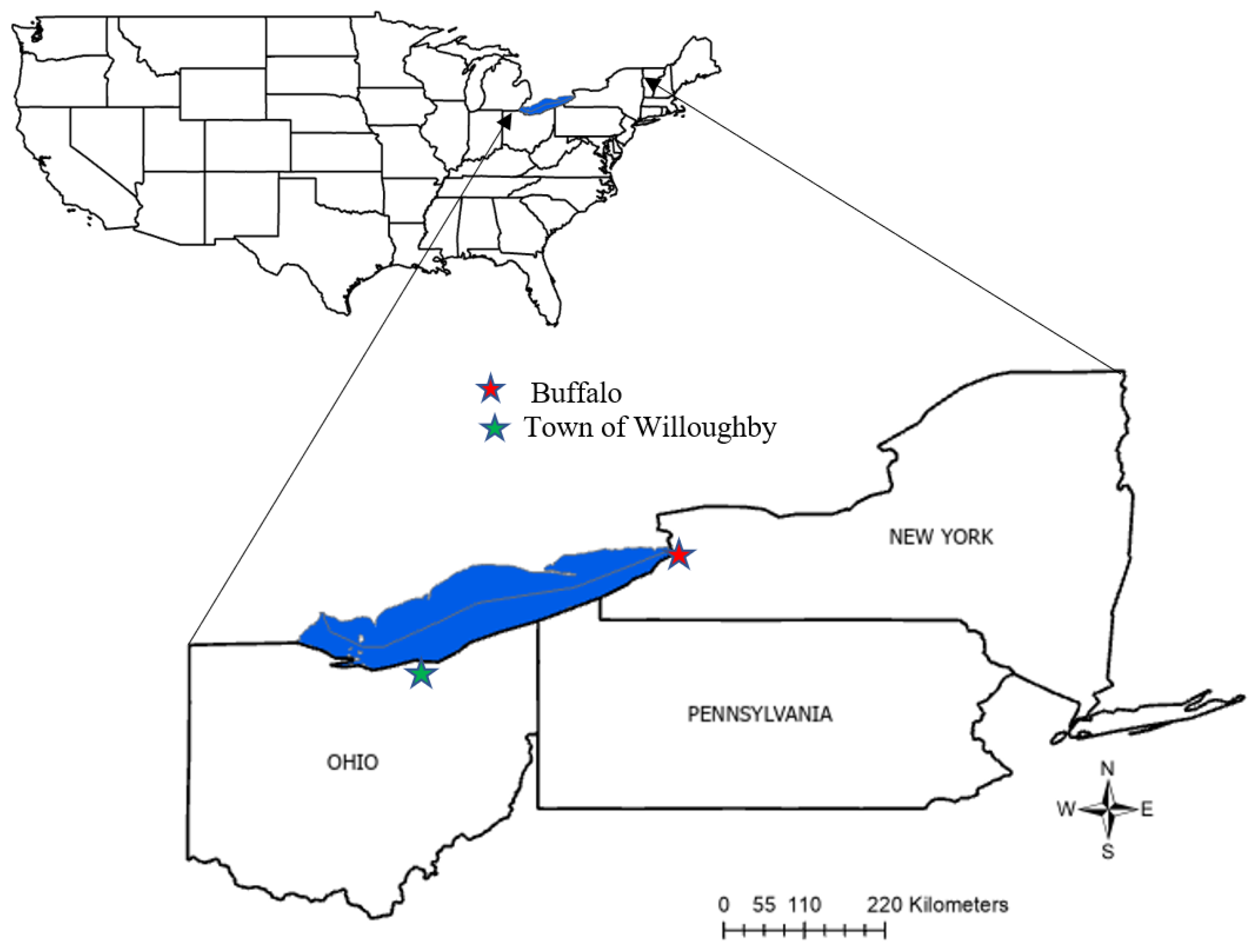
3.1. Study Area

The Lake Erie region, encompassing the towns of Willoughby in Lake County, Ohio, and Buffalo in Erie County, New York, presents a dynamic climate characterized by distinct seasonal variations and notable precipitation patterns (Figure 1). This geographical area, located in the United States, is situated along the eastern edge of the Great Lakes. The region’s climatic conditions and precipitation trends have been the focus of investigation, revealing important insights into changing weather dynamics.
Willoughby is nestled within Lake County, Ohio, and boasts geographical coordinates of 41°38′45″ N latitude and 81°24′35″ W longitude. Covering an area of 26.78 km2, with 26.55 km2 of land and 0.23 km2 of water, the town showcases a blend of natural and aquatic surroundings. The climate of Willoughby exhibits a clear division between its hot, muggy summers and cold, snowy winters. During the warm season, average daily high temperatures soar above 23 °C, peaking at around 28 °C, while lows hover around 20 °C. In contrast, the cold season sees average daily highs of 7 °C with lows plunging to −5 °C, and the high temperatures barely reaching 2 °C. Rainfall is a consistent feature throughout the year, with September holding the record for the wettest month, experiencing an average of 78mm of rain. In contrast, February marks the driest period with an average of 29 mm of rain. This climatic data, meticulously recorded from 2015 to 2023, provides a comprehensive understanding of Willoughby’s distinctive weather patterns. The region has witnessed an increase in temperature and rainfall intensity, coupled with a rising trend in extreme weather events, as documented in historical climate data [81].
Similarly, Buffalo, situated in Erie County, New York, is another integral part of the Lake Erie region (Figure 1). The city is positioned at 42°53′11″ N latitude and 78°52′41″ W longitude, encompassing an expansive area of 26.78 km2. Buffalo’s climate exhibits a distinct contrast between its warm, partly cloudy summers and its freezing, snowy, windy, and mostly cloudy winters. The warm season witnesses average daily high temperatures exceeding 21 °C, peaking at approximately 26 °C, while daily lows stay above 18 °C. In the cold season, average daily high temperatures barely reach 5°C, with lows plummeting to −6 °C and highs only reaching −0 °C. Like Willoughby, Buffalo experiences consistent rainfall throughout the year. September stands as the wettest month, with an average of 72 mm of rain, while February represents the driest month, recording an average of 19 mm of rain. The meticulously recorded climate patterns from 2015 to 2023 provide an in-depth understanding of Buffalo’s unique meteorological characteristics (Weather Spark).

3.2. Climate Model Data

Past observed precipitation as well as RCM and GCM output data for different models from CMIP5 and CMIP6, respectively, are included in the precipitation data used with historical data and future data under various scenarios. For the town of Willoughby, the historical observations were collected from the Hopkins International Airport station in Cleveland, Ohio, which is 50 km away from the study site.
Similarly, for Buffalo, the observed historical precipitation data were obtained from Buffalo Niagara International Airport. The 1 h precipitation data from the station were utilized to prepare the observed historical data. This station was selected because it provides long records of continuous data sets without any significant interruption.
The historical period from 1980–2019 was considered the baseline period and referred to as Time Span-1 (TS-1), whereas the future period was divided into two time spans 2020–2059 as the near future (TS-2), and 2060–2099 as the far future (TS-3). This was intended because the most recent data were available for the period of 1980–2019 and separating the future period into smaller time frames would allow for a more detailed analysis of potential changes in precipitation patterns with equal time for the near future and distant future, providing a more comprehensive and holistic view of the potential changes in precipitation patterns over time.
For this study, three RCMs with model-generated historical data and RCP8.5 scenarios for each CMIP5 were selected from https://na-cordex.org/, accessed on 1 January 2022. Similarly, for CMIP5, three GCMs with historical and four SSP scenarios, namely, SSP126, SSP245, SSP370, and SSP585, were chosen to examine the potential increase in future precipitation. The projected simulations of precipitation in the future were obtained from three climate models contributing to CMIP6: https://esgf-node.llnl.gov/search/cmip6/, accessed on 1 January 2022. Together, the four CMIP6 scenarios and RCP8.5 from CMIP5 provide historical background and future predictions for the study, with the former serving as a historical baseline for the worst-case climatic scenario and the latter as an attempt to give insights into possible future orientations. The fundamental information for the three selected CMIP5 and CMIP6 models is reported in Table 1.
The ability of the climate models to contribute hourly data was a primary factor in their selection for this study. In addition, these models have already been widely adopted in the research community, ensuring comparability and consistency with the existing literature and increasing the credibility and reliability of the research. Furthermore, a more noted comprehension of the potential effects of climate change on precipitation patterns was made possible by including both historical and different future scenarios. Such climate scenarios help us understand how precipitation responds to changes in greenhouse gas emissions, which is useful for planning responses to climate change.

3.3. Bias Correction of Raw Data

In this study, the climate data from the climate model were corrected against the observed daily data using the quantile mapping bias-correction approach, also known as probability mapping or distribution mapping.
In this study, the Climate Data Bias Corrector (CDBC) tool developed by Gupta et al. 2019 [82] was used to complete the bias correction. The effectiveness of the tool and its efficacy for bias corrections have been demonstrated in various studies [83,84,85,86,87].

3.4. Development of the IDF Curve

After the raw climate model data were bias-corrected, the next step was to develop an IDF curve using the Gumbel Extreme Distribution method. For this, the raw data were analyzed to determine the maximum precipitation intensity for each year from 1980 to 2099 for different rainfall durations (1 h, 2 h, 6 h, 12 h, and 24 h) at various return periods including 2, 5, 10, 25, 50, and 100 years. For each return period, the intensity of the precipitation for each duration was calculated using the average of the maximum precipitation and the standard deviation corresponding to the time frame. In addition, the Gumbel frequency factor, or K-factor, was used to calculate the probability of the occurrence of an event of a given magnitude.
Finally, the IDF curves were developed by plotting the intensity of precipitation against the duration of the rainfall for each return period using the Multi-Model Ensemble (MME) mean method.

4. Results and Discussion

Since the major objective of this study was to develop IDF curves for both CMIP5 and CMIP6 models and evaluate the differences between them, simulated precipitation data for historical and future periods were used. The data were adjusted to reduce biases using the quantile mapping approach, and the results of the bias correction process are presented in terms of the mean and standard deviation. The comparison of the average and variability (standard deviation) in both the CMIP5 and CMIP6 models, both before and after bias correction for the towns of Willoughby and Buffalo, has been presented in Table 2 and Table 3, respectively.

4.1. CMIP5

A comprehensive analysis of the IDF curves, assembling three CMIP5 models for the RCP8.5 scenario, provides a visual and mathematical representation of the changes in IDF. The IDF curve for the historical baseline period and the near future is presented in Figure 2. The analysis has revealed a considerable rise in rainfall intensity in the near future compared to the historical baseline period, with a projection of 9–39% for various durations and return periods for the town of Willoughby while the results from Buffalo demonstrated an elevation projecting an increase of 4% to 27% across various durations and return periods. It is important to note that the percentage increase was not linear, rather large variations were detected for longer durations and higher return periods. The non-linear nature of the increase in rainfall intensity implies that extreme rainfall events are projected to become even more intense in the near future. The analysis of the trend of precipitation indicated that the increasing pattern observed in the near future could be expected to further increase in the far future, as shown in Figure 3. Precipitation is expected to become more intense and increase by 20–55% compared to the historical baseline period for the town of Willoughby. However, such projections for the Buffalo region were relatively more and indicated a potential surge in precipitation intensity by 38% to 84% relative to the baseline historical period. Instances of extreme rainfall, both in shorter and longer return periods, have surged in both frequency and intensity. This tendency raises concerns about the likelihood of more frequent flash floods and stormwater flooding in the future. To further illustrate this point, Figure 4 presents a graphical comparison of the percentage change in intensity between different time frames. The study revealed that until the final years of the century, hourly precipitation with a 100-year return period would increase by almost 24% and 53% for the town of Willoughby and Buffalo region, respectively. Hourly precipitation intensity could be expected to follow a predictable trend, increasing by 16% in the near future and by a much larger percentage (29%) in the far future for the town of Willoughby while Buffalo exhibited a 17% elevation in the near future and a notably larger increment of 38% in the far future. These divergent tendencies highlight the value of looking across multiple time periods when analyzing climate projections for the future, which provide important clues that help us piece together how precipitation patterns may shift over time. This increasing trend of precipitation in the Lake Erie region that we found in our study is consistent with the findings of previous research [88,89] on the Great Lakes region using CMIP5 models. Notably, the same models were used in the former studies, which suggests the consistency and reliability of our findings.

4.2. CMIP6

In this study, the most recent climate model, CMIP6, agreed with the earlier versions of the model, i.e., CMIP5, in predicting an increase in precipitation. The findings indicated that even with the lowest SSP scenario (SSP126), there would be an increase in rainfall intensity in the near future, with a range of 3–19% for the town of Willoughby and 4% to 54% for Buffalo (Figure 5). It is interesting to note that the magnitude of the increase in the intensity of rainfall could be expected to vary across different durations and return periods. For the town of Willoughby, the two-year return period for a six-hour rainfall showed the lowest percentage increase in intensity. On the other hand, the return period of 100 years for rainfall lasting 2 h showed the largest percentage increase in intensity. However, for the Buffalo region, the smallest increase could be expected for a 24 h rainfall with a 2-year return period, whereas the largest increment could be expected for a 100-year return period for a 2-h duration rainfall. This trend persists in the far future (Figure 6), with the most pronounced increase as high as 56% anticipated for the 1-h duration of a 100-year return period.
The precipitation intensity for the near future can be expected to rise primarily for shorter durations (Figure 7). Similarly, this trend can be expected for the far future (Figure 8) suggesting a significant future increase in precipitation intensity for both the town of Willoughby and Buffalo, especially for shorter durations. It is interesting to report that a shorter duration of precipitation could be expected significantly in the Buffalo region compared to Willoughby. Comparing the near-future and historical baseline, this study indicated that precipitation intensity might double in the near future and triple in the far future for various durations and return periods. This disparity in trends emphasizes the significance of evaluating various time segments when analyzing future climate projections, enabling a deeper understanding of the evolving patterns of precipitation.
Likewise, the SSP370 scenario predicted intriguing insights about the future of precipitation intensity. In particular, hourly precipitation with a return period of two years is predicted to increase in intensity, with the lowest observed increase of 5% (Figure 9). The most significant increase in intensity, however, is expected for the 2-h duration of precipitation with a 100-year return period, which is projected to increase by 22% for the town of Willoughby. However, for the Buffalo region, it is projected to rise significantly to as high as 55% for a 1-h duration for a 2-year return period in the near future and by 94% for a 100-year return period in the far future. Comparisons of IDF curves for SSP370 near-future and far-future further underscore these trends (Figure 10).
Earlier research in the Great Lakes region [90] found that CMIP6 models’ representations of precipitation would vary widely and contrast with those observed in real-world data sets. Nonetheless, the MIROC6 model used in this study agreed with the similar trend in increased precipitation presented by Minallah and Steiner, 2021 [91], indicating the reliability of the findings and validating the predictive ability of the model for future precipitation patterns.

4.3. CMIP5 vs. CMIP6: A Comparison

The comparison of the near future for both CMIP5 RCP8.5 and CMIP6 SSP585 has been presented in Figure 14. The study revealed that the increase in rainfall intensity for various duration hours and return periods for CMIP5 RCP8.5 and CMIP6 SSP585 was projected to be within the range of 9–39% and 20–55% for the near future and the far future, respectively, for the town of Willoughby, whereas much a higher range from 4% to 57% for near future, and 19% to 140% for far future could be expected in the Buffalo region across different durations and return periods. Similarly, Figure 15 shows the plots of the far future for both CMIPs, suggesting a significant increase in precipitation in Lake Erie in the future.
The CMIP6 models were assessed under various scenarios, including ssp126, ssp245, ssp370, and ssp585, revealing an increase in precipitation intensity from 2–22% for the near future and 6–40% for the far future across various rainfall durations and return periods for the town of Willoughby, whereas an increase in precipitation intensity from 2% to 95% for the near future and 3% to 192% for the far future was detected in the Buffalo region. Even though both CMIPs indicate an increase in precipitation intensity, the CMIP5 RCP8.5 stands out with a higher rainfall intensity than the CMIP6 SSP585, with an intensity range that exceeds the CMIP6 SSP585 by 28% across varying durations and return periods for the town of Willoughby. Interestingly, in the Buffalo region, the findings highlight the intriguing revelation that CMIP6 projects a more substantial increase in intensity for longer durations and higher return periods, a departure from CMIP5’s trend. Notably, CMIP6 SSP scenarios emphasize significant changes, particularly for the future towards the century’s end. Furthermore, the contrast between CMIP5 predictions for Willoughby and Buffalo, and CMIP6’s higher prediction in Buffalo, underscores the complex regional variability.
During the analysis of meteorological data in this study, it was found that the intensity of precipitation would increase with longer return periods. The hourly precipitation is expected to see an increase in the upper range of extreme values in the future, specifically for the 95th percentile. This means that the most severe precipitation events that happen only 5% of the time are likely to become more intense, with a projected increase in the 95th percentile range of 5% to 24%, and the average hourly rainfall in the near future and far future is expected to increase by 7–28% by both CMIPs, which is a signal that communities need to prepare for the impacts of extreme weather events and invest in measures to build more resilient communities in the face of a changing climate. The results show that extreme weather events will become more intense, requiring sustainable development to mitigate urban flooding.
In Buffalo, the research foresees increased intensity of precipitation for extended return periods. The 95th percentile range, symbolizing severe rainfall events, is expected to triple in intensity by the century’s close, reflecting the escalating severity of extreme weather occurrences. There was a discrepancy between the study’s findings and the historical data reported by the National Oceanic and Atmospheric Administration (NOAA). One possible explanation for the discrepancies found in the data is that lakes were either simplified or left out entirely from the climate models used to examine potential future climate changes. The credibility of the CMIP5 models’ projections was called into question by a previous study by [91], which found that most of them did not accurately capture the impact of the Great Lakes on the regional climate. Inaccurately simulating regional climate patterns requires a thorough understanding of the interaction between lakes, the atmosphere, and the land. This highlights the need for additional research on the accuracy of sub-daily data and casts doubt on the applicability of the models used.
However, it is essential to acknowledge the limitations of this study, such as the fact that it is based on the rainfall estimates of a single location and may not be representative of every location of the Lake Erie basin. Further studies could be accomplished to explore the limitations and make improvements, such as potential uncertainties in the models, data, and bias correction methods. Regardless, the results of this study provide valuable insights for urban planners, engineers, and decision-makers in developing sustainable flood control measures to mitigate the limitations. Additionally, there is a chance that the bias correction methods adopted in this study, data, and models will all have uncertainties that will affect the results. Further studies may explore these limitations and improve upon them.

5. Conclusions

This study aimed to develop and compare the IDF curves for future climate scenarios using data from two different climate phases, CMIP5 and CMIP6, in the Lake Erie basin to evaluate the impact of climate change on rainfall intensity. Since IDF curves are essential tools in designing effective drainage systems for any engineering project, simulated precipitation data from historical and future periods were used to develop the IDF curves and make comparisons. The data were adjusted to reduce biases using the quantile mapping approach, and the bias-corrected climate data were used to develop the IDF curves using the Gumbel Extreme Distribution Type I method.
The results for the town of Willoughby indicated a rise in precipitation intensity in the future, ranging from 9 to 55% across different rainfall durations and return periods for CMIP5 RCP8.5 and CMIP6 SSP585. The analysis of CMIP6 climate scenarios predicted a significant average increase of 27% in the intensity of hourly precipitation for the recurrence interval of 100 years in the future. Specifically, the SSP585 scenario projected an increase of 9–26% in the near future and 21–47% in the far future, while the RCP8.5 scenario predicted an increase of 11% to 24%, respectively. Even under the moderate climate change scenario of SSP126, it can be expected to have an increase (averaging 6%) in hourly precipitation intensity with a 2-year return period.
Similarly, the results from Buffalo indicated a rise in precipitation intensity in the future, ranging from 3 to 140% across different rainfall durations and return periods for CMIP5 RCP8.5 and CMIP6 SSP585. The analysis of CMIP6 climate scenarios predicts a significant average increase of 99% in the intensity of hourly precipitation for the recurrence interval of 100 years in the future. Specifically, the SSP585 scenario projects an increase of 6 to 57% in the near future and 19 to 140% in the far future, while the RCP8.5 scenario predicts increases of 4% to 27% in the near future and 27% to 85% across varying rainfall duration and return periods, respectively. Even under the moderate climate change scenario of SSP126, it can be expected to have an increase (averaging 50%) in hourly precipitation intensity with a 2-year return period.
The reliance on a limited number of models and scenarios may not account for the entire range of uncertainty in future scenarios. By using a variety of models and scenarios, it is possible to ensure a thorough representation of climate projections, which successfully addresses issues with the overestimation or underestimation of climate consequences. This approach reduces biases promoting particular climatic outcomes, improving the study’s generalizability across different contexts and periods. In this context, further research is needed to understand the combined effects of these uncertainties with other sources of variability, such as land use change and natural internal weather variability. The large uncertainty is the output of the GCMs, and the RCMs also highlight the need for uncertainty analysis and probability-based IDF curves. Furthermore, the process of bias correction in a climate model is not immune to uncertainties. Climate scientists generally agree that extreme precipitation is intensifying; nevertheless, the phenomenon is complex and depends on a number of elements, including scale dependencies, physical considerations, regional variances, and confidence levels. To get accurate and trustworthy results for climate adaptation and infrastructure development, these aspects must be carefully taken into account during bias-correction processes. Future forecasts of climatic variables may be subjected to uncertainty after being corrected for bias in climate models, even when based on a single reference period. Hence, future climate results may vary depending on the reference period selected. These uncertainties impact research outcomes as they attempt to rectify inaccuracies in the data. The assumptions made during the correction process significantly influence the results and the manner in which data are rectified. Flaws in past data can lead to inaccuracies in future climate forecasts. Uncertainties arise when adjustments are made to data geographically or over different time spans. Different model responses to bias correction can leave behind residual errors. Additionally, in a changing environment, maintaining consistent climatic conditions becomes challenging, complicating future projections. Future research could explore various methods for responding to all these unknowns, such as using the professional analysis of climatologists or utilizing more robust statistical methods or machine learning algorithms. Therefore, in order to improve the current IDF curves in water infrastructure design, it is recommended that many time periods be taken into account in order to accommodate both immediate and long-term demands. In order to achieve dependable IDF curves, it is imperative to emphasize the implementation of strong statistical approaches in the processing of climatic data and bias correction. Furthermore, there is a need for a hybrid approach that makes use of many reference periods due to the complex nature of the interrelationships between climatic variables. To sum up, the study emphasizes the importance of updating the existing IDF curves that guide the design of water management infrastructure to account for the effects of climate change. It makes a substantial contribution to our understanding of how climate change impacts water management by providing information on shifting patterns of rainfall that are essential for developing adaptive infrastructure. The integration of many climate models and scenarios facilitates the development of adaptable infrastructure that can account for a range of potential outcomes. Concentrating on particular regions highlights the significance of customized planning for a range of climate impacts, and addressing uncertainties highlights the necessity of flexible infrastructure to handle a range of future possibilities, guaranteeing long-term climate preparedness.

Author Contributions

S.M. conducted an analysis and prepared the draft. S.S. provided a direction for the research and helped with the analysis and writing the manuscript. All authors have read and agreed to the published version of the manuscript.

Funding

This research was funded by Ohio Sea Grant.

Data Availability Statement

Data can be obtained with a request to the authors.

Acknowledgments

The authors would like to acknowledge Keely Davidson-Bennett from Chagrin River Watershed Partners (CRWP) for sharing her ideas and knowledge about the IDF curve of the region.

Conflicts of Interest

The authors declare no conflict of interest.

References

  1. IPCC. Climate Change 2007: Synthesis Report Summary for Policymakers; An Assessment of the Intergovernmental Panel on Climate Change; IPCC: Geneva, Switzerland, 2007. [Google Scholar]
  2. IPCC. Climate Change 2014: Synthesis Report; Longer Report; IPCC: Geneva, Switzerland, 2014. [Google Scholar]
  3. Allen, M.R.; Ingram, W.J. Insight Review Articles 224. 2002. Available online: www.nature.com/nature (accessed on 1 January 2022).
  4. Swain, D.L.; Wing, O.E.J.; Bates, P.D.; Done, J.M.; Johnson, K.A.; Cameron, D.R. Increased Flood Exposure Due to Climate Change and Population Growth in the United States. Earth’s Future 2020, 8, e2020EF001778. [Google Scholar] [CrossRef]
  5. Tabari, H. Climate change impact on flood and extreme precipitation increases with water availability. Sci. Rep. 2020, 10, 13768. [Google Scholar] [CrossRef] [PubMed]
  6. Trenberth, K.E.; Dai, A.; Rasmussen, R.M.; Parsons, D.B. The Changing character of precipitation. Bull. Am. Meteorol. Soc. 2003, 84, 1205–1218. [Google Scholar] [CrossRef]
  7. Haerter, J.O.; Berg, P. Unexpected rise in extreme precipitation caused by a shift in rain type? Nat. Geosci. 2009, 2, 372–373. [Google Scholar] [CrossRef]
  8. Lenderink, G.; Van Meijgaard, E. Increase in hourly precipitation extremes beyond expectations from temperature changes. Nat. Geosci. 2008, 1, 511–514. [Google Scholar] [CrossRef]
  9. Westra, S.; Fowler, H.J.; Evans, J.P.; Alexander, L.V.; Berg, P.; Johnson, F.; Kendon, E.J.; Lenderink, G.; Roberts, N.M. Future changes to the intensity and frequency of short-duration extreme rainfall. In Reviews of Geophysics; Blackwell Publishing Ltd.: Hoboken, NJ, USA, 2014; Volume 52, pp. 522–555. [Google Scholar] [CrossRef]
  10. Prein, A.F.; Rasmussen, R.M.; Ikeda, K.; Liu, C.; Clark, M.P.; Holland, G.J. The future intensification of hourly precipitation extremes. Nat. Clim. Chang. 2017, 7, 48–52. [Google Scholar] [CrossRef]
  11. Easterling, D.R.; Meehl, G.A.; Parmesan, C.; Changnon, S.A.; Karl, T.R.; Mearns, L.O. Climate Extremes: Observations, Modeling, and Impacts. Science 2000, 289, 2068–2074. [Google Scholar] [CrossRef]
  12. Groisman, P.Y.; Knight, R.W.; Easterling, D.R.; Karl, T.R.; Hegerl, G.C.; Razuvaev, V.N. Trends in Intense Precipitation in the Climate Record. J. Clim. 2005, 18, 1326–1350. [Google Scholar] [CrossRef]
  13. Kourtis, I.M.; Tsihrintzis, V.A. Update of intensity-duration-frequency (IDF) curves under climate change: A review. Water Supply 2022, 22, 4951–4974. [Google Scholar] [CrossRef]
  14. Cook, L.M.; McGinnis, S.; Samaras, C. The effect of modeling choices on updating intensity-duration-frequency curves and stormwater infrastructure designs for climate change. Clim. Chang. 2020, 159, 289–308. [Google Scholar] [CrossRef]
  15. Thakali, R.; Kalra, A.; Ahmad, S. Understanding the effects of climate change on urban stormwater infrastructures in the Las Vegas Valley. Hydrology 2016, 3, 34. [Google Scholar] [CrossRef]
  16. Guo, Y.; Asce, M. Updating Rainfall IDF Relationships to Maintain Urban Drainage Design Standards. J. Hydrol. Eng. 2006, 11, 506–509. [Google Scholar] [CrossRef]
  17. Liu, L. The dynamics of early-stage transmission of COVID-19: A novel quantification of the role of global temperature. Gondwana Res. 2023, 114, 55–68. [Google Scholar] [CrossRef] [PubMed]
  18. Martel, J.-L.; Brissette, F.P.; Lucas-Picher, P.; Troin, M.; Arsenault, R. Climate Change and Rainfall Intensity–Duration–Frequency Curves: Overview of Science and Guidelines for Adaptation. J. Hydrol. Eng. 2021, 26, 03121001. [Google Scholar] [CrossRef]
  19. Mohammed, A.; Dan’Azumi, S.; Modibbo, A.A.; Adamu, A.A. Development of Rainfall Intensity Duration Frequency (IDF) Curves for Design of Hydraulic Structures in Kano State, Nigeria. Platform 2021, 5, 10–22. [Google Scholar]
  20. Elsebaie, I.H. Developing rainfall intensity–duration–frequency relationship for two regions in Saudi Arabia. J. King Saud Univ.-Eng. Sci. 2012, 24, 131–140. [Google Scholar] [CrossRef]
  21. Kundwa, M.J. Development of Rainfall Intensity Duration Frequency (IDF) Curves for Hydraulic Design Aspect. J. Ecol. Nat. Resour. 2019, 3, 1–14. [Google Scholar] [CrossRef]
  22. Rashid, M.; Faruque, S.; Rashid, M.M.; Faruque, S.B.; Alam, J.B. Modeling of Short Duration Rainfall Intensity Duration Frequency (SDR-IDF) Equation for Sylhet City in Bangladesh Statistical Downscaling of GCM Outputs to Rainfall View Project Extreme Sea Level Variations along the U.S. Coastlines View Project Modeling of Short Duration Rainfall Intensity Duration Frequency (SDR-IDF) Equation for Sylhet City in Bangladesh. 2. 2012. Available online: http://www.ejournalofscience.org (accessed on 1 January 2022).
  23. Singh, R.; Arya, D.S.; Taxak, A.K.; Vojinovic, Z. Potential Impact of Climate Change on Rainfall Intensity-Duration-Frequency Curves in Roorkee, India. Water Resour. Manag. 2016, 30, 4603–4616. [Google Scholar] [CrossRef]
  24. Prodanovic, P.; Simonovic, S.P. The university of western ontario department of civil and environmental engineering. In Water Resources Research Report; John Wiley & Sons: Hoboken, NJ, USA, 2007. [Google Scholar]
  25. Srivastav, R.K.; Schardong, A.; Simonovic, S.P. Equidistance Quantile Matching Method for Updating IDFCurves under Climate Change. Water Resour. Manag. 2014, 28, 2539–2562. [Google Scholar] [CrossRef]
  26. Hess, J.J.; Malilay, J.N.; Parkinson, A.J. Climate Change. The Importance of Place. Am. J. Prev. Med. 2008, 35, 468–478. [Google Scholar] [CrossRef]
  27. Hosseinzadehtalaei, P.; Tabari, H.; Willems, P. Climate change impact on short-duration extreme precipitation and intensity–duration–frequency curves over Europe. J. Hydrol. 2020, 590, 125249. [Google Scholar] [CrossRef]
  28. Peck, A.; Prodanovic, P.; Simonovic, S.P. Rainfall intensity duration frequency curves under climate change: City of London, Ontario, Canada. Can. Water Resour. J. 2012, 37, 177–189. [Google Scholar] [CrossRef]
  29. Trenberth, K.E. Changes in precipitation with climate change. Clim. Res. 2011, 47, 123–138. [Google Scholar] [CrossRef]
  30. Rodríguez, R.; Navarro, X.; Casas, M.C.; Ribalaygua, J.; Russo, B.; Pouget, L.; Redaño, A. Influence of climate change on IDF curves for the metropolitan area of Barcelona (Spain). Int. J. Climatol. 2014, 34, 643–654. [Google Scholar] [CrossRef]
  31. Shrestha, A.; Babel, M.S.; Weesakul, S.; Vojinovic, Z. Developing Intensity-Duration-Frequency (IDF) curves under climate change uncertainty: The case of Bangkok, Thailand. Water 2017, 9, 145. [Google Scholar] [CrossRef]
  32. Shrestha, S.; Sharma, S. Assessment of climate change impact on high flows in a watershed characterized by flood regulating reservoirs. Int. J. Agric. Biol. Eng. 2021, 14, 178–191. [Google Scholar] [CrossRef]
  33. Ghasemi Tousi, E.; O’Brien, W.; Doulabian, S.; Shadmehri Toosi, A. Climate changes impact on stormwater infrastructure design in Tucson Arizona. Sustain. Cities Soc. 2021, 72, 103014. [Google Scholar] [CrossRef]
  34. Lopez-Cantu, T.; Prein, A.F.; Samaras, C. Uncertainties in Future U.S. Extreme Precipitation from Downscaled Climate Projections. Geophys. Res. Lett. 2020, 47, e2019GL086797. [Google Scholar] [CrossRef]
  35. Chen, H.; Sun, J.; Lin, W.; Xu, H. Comparison of CMIP6 and CMIP5 models in simulating climate extremes. In Science Bulletin; Elsevier B.V.: Amsterdam, The Netherlands, 2020; Volume 65, pp. 1415–1418. [Google Scholar] [CrossRef]
  36. Thibeault, J.M.; Seth, A. Changing climate extremes in the Northeast United States: Observations and projections from CMIP5. Clim. Chang. 2014, 127, 273–287. [Google Scholar] [CrossRef]
  37. Ragno, E.; AghaKouchak, A.; Love, C.A.; Cheng, L.; Vahedifard, F.; Lima, C.H.R. Quantifying Changes in Future Intensity-Duration-Frequency Curves Using Multimodel Ensemble Simulations. Water Resour. Res. 2018, 54, 1751–1764. [Google Scholar] [CrossRef]
  38. Cheng, L.; Aghakouchak, A. Nonstationary precipitation intensity-duration-frequency curves for infrastructure design in a changing climate. Sci. Rep. 2014, 4, 7093. [Google Scholar] [CrossRef] [PubMed]
  39. Coelho, G.d.A.; Ferreira, C.M.; Johnston, J.; Kinter, J.L.; Dollan, I.J.; Maggioni, V. Potential Impacts of Future Extreme Precipitation Changes on Flood Engineering Design Across the Contiguous United States. Water Resour. Res. 2022, 58, e2021WR031432. [Google Scholar] [CrossRef]
  40. Lee, J.W.; Hong, S.Y.; Chang, E.C.; Suh, M.S.; Kang, H.S. Assessment of future climate change over East Asia due to the RCP scenarios downscaled by GRIMs-RMP. Clim. Dyn. 2014, 42, 733–747. [Google Scholar] [CrossRef]
  41. Rummukainen, M. Added value in regional climate modeling. Wiley Interdiscip. Rev. Clim. Chang. 2016, 7, 145–159. [Google Scholar] [CrossRef]
  42. Park, J.H.; Oh, S.G.; Suh, M.S. Impacts of boundary conditions on the precipitation simulation of RegCM4 in the CORDEX East Asia domain. J. Geophys. Res. Atmos. 2013, 118, 1652–1667. [Google Scholar] [CrossRef]
  43. Qian, Y.; Ghan, S.J.; Leung, L.R. Downscaling hydroclimatic changes over the western US based on CAM subgrid scheme and WRF regional climate simulations. Int. J. Climatol. 2010, 30, 675–693. [Google Scholar] [CrossRef]
  44. O’Neill, B.C.; Tebaldi, C.; Van Vuuren, D.P.; Eyring, V.; Friedlingstein, P.; Hurtt, G.; Knutti, R.; Kriegler, E.; Lamarque, J.F.; Lowe, J.; et al. The Scenario Model Intercomparison Project (ScenarioMIP) for CMIP6. Geosci. Model Dev. 2016, 9, 3461–3482. [Google Scholar] [CrossRef]
  45. Giorgi, F.; Jones, C.; Asrar, G.R. Addressing climate information needs at the regional level: The CORDEX framework. WMO Bull. 2009, 58, 175. [Google Scholar]
  46. Gutowski, J.W.; Giorgi, F.; Timbal, B.; Frigon, A.; Jacob, D.; Kang, H.S.; Raghavan, K.; Lee, B.; Lennard, C.; Nikulin, G.; et al. WCRP COordinated Regional Downscaling EXperiment (CORDEX): A diagnostic MIP for CMIP6. Geosci. Model Dev. 2016, 9, 4087–4095. [Google Scholar] [CrossRef]
  47. McGinnis, S.; Mearns, L. Building a climate service for North America based on the NA-CORDEX data archive. Clim. Serv. 2021, 22, 100233. [Google Scholar] [CrossRef]
  48. Gutowski, W.J.; Ullrich, P.A.; Hall, A.; Leung, L.R.; O’Brien, T.A.; Patricola, C.M.; Arritt, R.W.; Bukovsky, M.S.; Calvin, K.V.; Feng, Z.; et al. The ongoing need for high-resolution regional climate models: Process understanding and stakeholder information. Bull. Am. Meteorol. Soc. 2021, 101, E664–E683. [Google Scholar] [CrossRef]
  49. Kirtman, B.; Pirani, A. The State of the Art of Seasonal Prediction: Outcomes and Recommendations from the First World Climate Research Program Workshop on Seasonal Prediction. Bull. Am. Meteorol. Soc. 2009, 90, 455–458. [Google Scholar] [CrossRef]
  50. Moss, R.H.; Edmonds, J.A.; Hibbard, K.A.; Manning, M.R.; Rose, S.K.; van Vuuren, D.P.; Carter, T.R.; Emori, S.; Kainuma, M.; Kram, T.; et al. The next generation of scenarios for climate change research and assessment. Nature 2010, 463, 747–756. [Google Scholar] [CrossRef] [PubMed]
  51. Bruyère, C.L.; Done, J.M.; Holland, G.J.; Fredrick, S. Bias corrections of global models for regional climate simulations of high-impact weather. Clim. Dyn. 2014, 43, 1847–1856. [Google Scholar] [CrossRef]
  52. Donat, M.G.; Lowry, A.L.; Alexander, L.V.; O’Gorman, P.A.; Maher, N. More extreme precipitation in the worldâ €TM s dry and wet regions. Nat. Clim. Chang. 2016, 6, 508–513. [Google Scholar] [CrossRef]
  53. Gao, X.-J.; Wang, M.-L.; Giorgi, F. Climate Change over China in the 21st Century as Simulated by BCC_CSM1.1-RegCM4.0. Atmos. Ocean. Sci. Lett. 2013, 6, 381–386. [Google Scholar] [CrossRef]
  54. Maraun, D.; Shepherd, T.G.; Widmann, M.; Zappa, G.; Walton, D.; Gutiérrez, J.M.; Hagemann, S.; Richter, I.; Soares, P.M.M.; Hall, A.; et al. Towards process-informed bias correction of climate change simulations. Nat. Clim. Chang. 2017, 7, 764–773. [Google Scholar] [CrossRef]
  55. Mehrotra, R.; Sharma, A. An improved standardization procedure to remove systematic low frequency variability biases in GCM simulations. Water Resour. Res. 2012, 48. [Google Scholar] [CrossRef]
  56. Xu, Z.; Yang, Z.L. An improved dynamical downscaling method with GCM bias corrections and its validation with 30 years of climate simulations. J. Clim. 2012, 25, 6271–6286. [Google Scholar] [CrossRef]
  57. Acharya, N.; Chattopadhyay, S.; Mohanty, U.C.; Dash, S.K.; Sahoo, L.N. On the bias correction of general circulation model output for Indian summer monsoon. Meteorol. Appl. 2013, 20, 349–356. [Google Scholar] [CrossRef]
  58. Wood, A.W.; Leung, L.R.; Sridhar, V.; Lettenmaier, D.P. Hydrologic Implications of dynamical and statistical approaches to downscaling climate model outputs. Clim. Chang. 2004, 62, 189–216. [Google Scholar] [CrossRef]
  59. Abatzoglou, J.T.; Brown, T.J. A comparison of statistical downscaling methods suited for wildfire applications. Int. J. Climatol. 2012, 32, 772–780. [Google Scholar] [CrossRef]
  60. Chen, J.; Brissette, F.P.; Chaumont, D.; Braun, M. Finding appropriate bias correction methods in downscaling precipitation for hydrologic impact studies over North America. Water Resour. Res. 2013, 49, 4187–4205. [Google Scholar] [CrossRef]
  61. Gudmundsson, L.; Bremnes, J.B.; Haugen, J.E.; Engen-Skaugen, T. Technical Note: Downscaling RCM precipitation to the station scale using statistical transformations – A comparison of methods. Hydrol. Earth Syst. Sci. 2012, 16, 3383–3390. [Google Scholar] [CrossRef]
  62. Maraun, D. Bias Correcting Climate Change Simulations—A Critical Review. In Current Climate Change Reports; Springer: Berlin/Heidelberg, Germany, 2016; Volume 2, pp. 211–220. [Google Scholar] [CrossRef]
  63. Maraun, D.; Wetterhall, F.; Ireson, A.M.; Chandler, R.E.; Kendon, E.J.; Widmann, M.; Brienen, S.; Rust, H.W.; Sauter, T.; Themel, M.; et al. Precipitation downscaling under climate change: Recent developments to bridge the gap between dynamical models and the end user. Rev. Geophys. 2010, 48, 1–34. [Google Scholar] [CrossRef]
  64. Pierce, D.W.; Cayan, D.R.; Thrasher, B.L. Statistical Downscaling Using Localized Constructed Analogs (LOCA). J. Hydrometeorol. 2014, 15, 2558–2585. [Google Scholar] [CrossRef]
  65. Tabari, H.; Paz, S.M.; Buekenhout, D.; Willems, P. Comparison of statistical downscaling methods for climate change impact analysis on precipitation-driven drought. Hydrol. Earth Syst. Sci. 2021, 25, 3493–3517. [Google Scholar] [CrossRef]
  66. Grose, M.R.; Post, D.A.; Ling, F.L.N.; Corney, S.; Bennett, J.C.; Grose, M.R.; Post, D.A.; Ling, F.L.N.; Corney, S.P.; Bindoff, N.L. Performance of Quantile-Quantile Bias-Correction for Use in Hydroclimatological Projections Bioregional Assessment Programme View Project Barwon Water Inflows under Climate Change View Project Performance of Quantile-Quantile Bias-correction for Use in Hydroclimatological Projections. 2011. Available online: http://mssanz.org.au/modsim2011 (accessed on 1 January 2022).
  67. Hayhoe, K.; Wake, C.; Anderson, B.; Liang, X.Z.; Maurer, E.; Zhu, J.; Bradbury, J.; Degaetano, A.; Stoner, A.M.; Wuebbles, D. Regional climate change projections for the Northeast USA. Mitig. Adapt. Strateg. Glob. Chang. 2008, 13, 425–436. [Google Scholar] [CrossRef]
  68. Maurer, E.P.; Duffy, P.B. Uncertainty in projections of streamflow changes due to climate change in California. Geophys. Res. Lett. 2005, 32, 1–5. [Google Scholar] [CrossRef]
  69. Li, H.; Sheffield, J.; Wood, E.F. Bias correction of monthly precipitation and temperature fields from Intergovernmental Panel on Climate Change AR4 models using equidistant quantile matching. J. Geophys. Res. Atmos. 2010, 115. [Google Scholar] [CrossRef]
  70. Maurer, E.P.; Pierce, D.W. Bias correction can modify climate model simulated precipitation changes without adverse effect on the ensemble mean. Hydrol. Earth Syst. Sci. 2014, 18, 915–925. [Google Scholar] [CrossRef]
  71. Obaid, N.; Alghazali, S.; Adnan, D.; Alawadi, H. Fitting Statistical Distributions of Monthly Rainfall for Some Iraqi Stations. Civ. Environ. Res. 2014, 6, 40–46. [Google Scholar]
  72. AlHassoun, S.A. Developing an empirical formulae to estimate rainfall intensity in Riyadh region. J. King Saud Univ.-Eng. Sci. 2011, 23, 81–88. [Google Scholar] [CrossRef]
  73. Hailegeorgis, T.T.; Thorolfsson, S.T.; Alfredsen, K. Regional frequency analysis of extreme precipitation with consideration of uncertainties to update IDF curves for the city of Trondheim. J. Hydrol. 2013, 498, 305–318. [Google Scholar] [CrossRef]
  74. Al Islam, M.; Hasan, H. Generation of IDF equation from catchment delineation using GIS. Civ. Eng. J. 2020, 6, 540–547. [Google Scholar] [CrossRef]
  75. Mujere, N. Flood Frequency Analysis Using the Gumbel Distribution. Int. J. Comput. Sci. Eng. 2011, 3, 2774–2778. [Google Scholar]
  76. Solomon, O.; Prince, O. Flood Frequency Analysis of Osse River Using Gumbel’s Distribution. Civ. Environ. Res. 2013, 3, 55–59. [Google Scholar]
  77. Vidal, I. A Bayesian analysis of the Gumbel distribution: An application to extreme rainfall data. Stoch. Environ. Res. Risk Assess. 2014, 28, 571–582. [Google Scholar] [CrossRef]
  78. Tahir, W.; Bakar, S.H.A.; Wahid, M.A.; Nasir, S.R.M.; Lee, W.K. ISFRAM 2015; Springer: Singapore, 2016. [Google Scholar] [CrossRef]
  79. Yong, S.L.S.; Ng, J.L.; Huang, Y.F.; Ang, C.K. Assessment of the best probability distribution method in rainfall frequency analysis for a tropical region. Malays. J. Civ. Eng. 2021, 33. [Google Scholar] [CrossRef]
  80. Balakrishnan, N.; Cramer, E.; Kundu, D. Hybrid Censoring Know-How: Designs and Implementations; Academic Press: Chicago, IL, USA, 2023. [Google Scholar]
  81. Bartels, R.J.; Black, A.W.; Keim, B.D. Trends in precipitation days in the United States. Int. J. Climatol. 2020, 40, 1038–1048. [Google Scholar] [CrossRef]
  82. Gupta, R.; Bhattarai, R.; Mishra, A. Development of climate data bias corrector (CDBC) tool and its application over the agro-ecological zones of India. Water 2019, 11, 1102. [Google Scholar] [CrossRef]
  83. Ayugi, B.; Shilenje, Z.W.; Babaousmail, H.; Lim Kam Sian, K.T.C.; Mumo, R.; Dike, V.N.; Iyakaremye, V.; Chehbouni, A.; Ongoma, V. Projected changes in meteorological drought over East Africa inferred from bias-adjusted CMIP6 models. Nat. Hazards 2022, 113, 1151–1176. [Google Scholar] [CrossRef] [PubMed]
  84. Babaousmail, H.; Ayugi, B.; Rajasekar, A.; Zhu, H.; Oduro, C.; Mumo, R.; Ongoma, V. Projection of Extreme Temperature Events over the Mediterranean and Sahara Using Bias-Corrected CMIP6 Models. Atmosphere 2022, 13, 741. [Google Scholar] [CrossRef]
  85. Babaousmail, H.; Hou, R.; Ayugi, B.; Sian, K.T.C.L.K.; Ojara, M.; Mumo, R.; Chehbouni, A.; Ongoma, V. Future changes in mean and extreme precipitation over the Mediterranean and Sahara regions using bias-corrected CMIP6 models. Int. J. Climatol. 2022, 42, 7280–7297. [Google Scholar] [CrossRef]
  86. Lim Kam Sian, K.T.C.; Hagan, D.F.T.; Ayugi, B.O.; Nooni, I.K.; Ullah, W.; Babaousmail, H.; Ongoma, V. Projections of precipitation extremes based on bias-corrected Coupled Model Intercomparison Project phase 6 models ensemble over southern Africa. Int. J. Climatol. 2022, 42, 8269–8289. [Google Scholar] [CrossRef]
  87. Shrestha, S.; Sharma, S.; Gupta, R.; Bhattarai, R. Impact of global climate change on stream low flows: A case study of the great Miami river Watershed, Ohio. Int. J. Agric. Biol. Eng. 2019, 12, 84–95. [Google Scholar] [CrossRef]
  88. Xue, P.; Ye, X.; Pal, J.S.; Chu, P.Y.; Kayastha, M.B.; Huang, C. Climate projections over the Great Lakes Region: Using two-way coupling of a regional climate model with a 3-D lake model. Geosci. Model Dev. 2022, 15, 4425–4446. [Google Scholar] [CrossRef]
  89. Zhang, L.; Zhao, Y.; Hein-Griggs, D.; Janes, T.; Tucker, S.; Ciborowski, J.J.H. Climate change projections of temperature and precipitation for the great lakes basin using the PRECIS regional climate model. J. Great Lakes Res. 2020, 46, 255–266. [Google Scholar] [CrossRef]
  90. Minallah, S.; Steiner, A.L. Analysis of the Atmospheric Water Cycle for the Laurentian Great Lakes Region Using CMIP6 Models. J. Clim. 2021, 34, 4693–4710. [Google Scholar] [CrossRef]
  91. Briley, L.J.; Rood, R.B.; Notaro, M. Large lakes in climate models: A Great Lakes case study on the usability of CMIP5. J. Great Lakes Res. 2021, 47, 405–418. [Google Scholar] [CrossRef]
Figure 1. The study area showing the two cities, the town of Willoughby and Buffalo, near the Lake Erie Coast.
Water 15 04063 g001
Figure 2. IDF curves for the baseline period from 1980 to 2019 (TS-1) vs. the near future from 2020 to 2059 (TS-2) considering a 2, 5, 10, 25, 50, and 100-year return period ensembling three CMIP5 RCP8.5 models for (a) the town of Willoughby (left panel), and (b) the city of Buffalo (right panel).
Water 15 04063 g002
Figure 3. IDF curves for the baseline period from 1980 to 2019 (TS-1) vs. the far-future period from 2060 to 2099 (TS-3) considering a 2, 5, 10, 25, 50, and 100-year return period ensembling three CMIP5 RCP8.5 models for (a) the town of Willoughby (left panel), and (b) the city of Buffalo (right panel).
Water 15 04063 g003
Figure 4. The left and right figures of the upper panel (a) represent the town of Willoughby, whereas the left and right figures of the lower panel (b) represent the city of Buffalo. The left graph of the upper panel shows the comparison of the percentage change in the rainfall intensity between the baseline period from 1980 to 2019 (TS-1) vs. the near future from 2020 to 2059 (TS-2), whereas the right panel shows the baseline period from 1980 to 2019 (TS-1) vs. the far future period from 2060 to 2099 (TS-3) for the town of Willoughby for different return periods and rainfall durations of CMIP5 RCP8.5. The exact interpretation is true for the city of Buffalo in the lower panel.
Water 15 04063 g004
Figure 5. IDF curves for the baseline period from 1980 to 2019 (TS-1) vs. the near future from 2020 to 2059 (TS-2) considering a 2, 5, 10, 25, 50, and 100-year return period ensembling three CMIP6 SSP126 models for (a) the town of Willoughby (left panel), (b) city of Buffalo (right panel).
Water 15 04063 g005
Figure 6. IDF curves for the baseline period from 1980 to 2019 (TS-1) vs. the far future from 2060 to 2099 (TS-3) considering a 2, 5, 10, 25, 50, and 100-year return period ensembling three CMIP6 SSP126 models for (a) the town of Willoughby (left panel), and (b) city of Buffalo (right panel).
Water 15 04063 g006
Figure 7. IDF curves for the baseline period from 1980 to 2019 (TS-1) vs. the near future from 2020 to 2059 (TS-2:) considering a 2, 5, 10, 25, 50, and 100-year return period ensembling three CMIP6 SSP245 models for (a) the town of Willougby (left panel), (b) city of Buffalo (right panel).
Water 15 04063 g007
Figure 8. IDF curves for the baseline period (TS-1: 1980–2019) vs. the far future (TS-3: 2060–2099) considering a 2, 5, 10, 25, 50, and 100-year return period ensembling three CMIP6 SSP245 models for (a) the town of Willoughby and (b) city of Buffalo.
Water 15 04063 g008
Figure 9. IDF curves for the baseline period (TS-1: 1980–2019) vs. the near future (TS-2: 2020–2059) considering a 2, 5, 10, 25, 50, and 100-year return period ensembling three CMIP6 SSP370 models for (a) the town of Willoughby (left panel) and (b) city of Buffalo (right panel).
Water 15 04063 g009
Figure 10. IDF curves for the baseline period (TS-1: 1980–2019) vs. the far future (TS-3: 2060–2099) considering a 2, 5, 10, 25, 50, and 100-year return period ensembling three CMIP6 SSP370 models for (a) the town of Willoughby (left panel) and (b) city of Buffalo (right panel). In the same manner, the SSP585 scenario under the CMIP6 model demonstrated an increase in precipitation intensity, with a projected range of 6–57% (Figure 11) and 19–140% (Figure 12) for the near-future and far-future, respectively, for various durations and return periods for both the town of Willoughby and the Buffalo region. The results showed that in the most catastrophic scenario (SSP585), hourly precipitation with a 100-year return period would rise by an average of approximately 24% in the future in the town of Willoughby and by around 80% in the Buffalo region (Figure 13).
Water 15 04063 g010
Figure 11. IDF curves for the baseline period from 1980 to 2019 (TS-1) vs. the near future from 2020 to 2059 (TS-2) considering a 2, 5, 10, 25, 50, and 100-year return period ensembling three CMIP6 SSP585 models for (a) the town of Willoughby (left panel) and (b) city of Buffalo (right panel).
Water 15 04063 g011
Figure 12. IDF curves for the baseline period from 1980 to 2019 (TS-1) vs. the far future from 2060 to 2099 (TS-3) considering a 2, 5, 10, 25, 50, and 100-year return period ensembling three CMIP6 SSP585 models for (a) the town of Willoughby (left panel), (b) city of Buffalo (right panel).
Water 15 04063 g012
Figure 13. The upper panel (a) represents the town of Willoughby and the lower panel (b) represents the City of Buffalo. The upper panel shows the graphical comparison showing the rainfall intensity percentage change between the baseline period from 1980 to 2019 (TS-1) vs. the near future from 2020 to 2059 (TS-2), on the left, and the baseline period from 1980 to 2019 (TS-1) vs. the far future from 2080 to 2099 (TS-3), on the right, for different return periods and rainfall duration of CMIP6 SSP585 in the upper panel for the town of Willoughby (a). The exact similar comparison is presented in the lower panel (b) for the city of Buffalo.
Water 15 04063 g013
Figure 14. IDF curves for the near future period from 2020 to 2059 (TS-2:) considering a 2, 5, 10, 25, 50, and 100-year return period ensembling three CMIP5 RCP8.5 vs. CMIP6 SSP585 models for (a) the town of Willoughby (left panel), and (b) city of Buffalo (right panel).
Water 15 04063 g014
Figure 15. IDF curves for the far future period from 2060 to 2099 (TS-3) considering a 2, 5, 10, 25, 50, and 100-year return period ensembling three CMIP5 RCP8.5 vs. CMIP6 SSP585 models for (a) the town of Willoughby (left panel), and (b) city of Buffalo (right panel).
Water 15 04063 g015
Table 1. Description of the climate models and climate change scenarios used in the study.
CMIP5
SourceSource IDGCMScenarioGridFrequencyResolution
NA-CORDEXWRFGFDL-ESM2Mhist, RCP8.5NAM-221 h0.44° × 0.44°
HadGEM2-ES
MPI-ESM-LR
CMIP6
SourceSource IDExperiment IDVariant LabelFrequencyResolution
WRCPMIROC6hist, ssp126, ssp245, ssp370, ssp585r1i1p1f11 h1.4° × 1.4°
CNRM-CM6-1-HRr1i1p1f20.5° × 0.5°
CNRM-ESM2-1r1i1p1f21.4° × 1.4°
Table 2. Bias in terms of mean and standard deviation (st. dev.) before and after bias correction for CMIP5 and CMIP6 models for the baseline period (TS-1: 1980–2019) for the town of Willoughby.
StatisticsCMIP5 Models
ObservedGFDL-ESM2MHadGEM2-ESMPI-ESM-LR
BeforeAfterBeforeAfterBeforeAfter
Average (mm)2.674.042.63.062.683.562.51
St. Dev. (mm)6.627.246.787.116.586.796.39
CMIP6 Models
StatisticsObservedGFDL-ESM2MHadGEM2-ESMPI-ESM-LR
BeforeAfterBeforeAfterBeforeAfter
Average (mm)2.673.042.693.362.653.302.68
St. Dev. (mm)6.626.066.776.606.716.136.77
Table 3. Bias in terms of mean and standard deviation (st. dev.) before and after bias correction for CMIP5 and CMIP6 models for the baseline period (TS-1: 1980–2019) for Buffalo.
StatisticsCMIP5 Models
ObservedGFDL-ESM2MHadGEM2-ESMPI-ESM-LR
BeforeAfterBeforeAfterBeforeAfter
Average (mm)1.973.651.933.842.174.012.35
St. Dev. (mm)5.407.065.667.646.528.057.23
CMIP6 Models
StatisticsObservedGFDL-ESM2MHadGEM2-ESMPI-ESM-LR
BeforeAfterBeforeAfterBeforeAfter
Average (mm)1.973.161.433.271.443.101.44
St. Dev. (mm)5.406.294.906.114.936.244.87
Disclaimer/Publisher’s Note: The statements, opinions and data contained in all publications are solely those of the individual author(s) and contributor(s) and not of MDPI and/or the editor(s). MDPI and/or the editor(s) disclaim responsibility for any injury to people or property resulting from any ideas, methods, instructions or products referred to in the content.

