Article

Effects of Decomposition of Submerged Aquatic Plants on CO2 and CH4 Release in River Sediment–Water Environment

1
Jiangsu Ecological Environmental Monitoring Co., Ltd., Nanjing 210036, China
2
Nanjing Institute of Environmental Sciences, Ministry of Ecology and Environment, Nanjing 210042, China
3
Jiangsu Key Laboratory of Atmospheric Environment Monitoring and Pollution Control (AEMPC), Collaborative Innovation Center of Atmospheric Environment and Equipment Technology (CIC-AEET), School of Environmental Science and Engineering, Nanjing University of Information Science & Technology, Nanjing 210044, China
*
Authors to whom correspondence should be addressed.
These authors contributed equally to this work.
Water 2023, 15(16), 2863; https://doi.org/10.3390/w15162863
Submission received: 18 April 2023 / Revised: 20 July 2023 / Accepted: 27 July 2023 / Published: 8 August 2023
(This article belongs to the Section Biodiversity and Functionality of Aquatic Ecosystems)

Abstract

:
Organic matter was increased due to the input of plant litter, resulting in changes in the physicochemical properties and enhancement of greenhouse gas (GHG) emissions in water bodies. There are few reports on effects of decomposition of aquatic plants on GHGs emissions. This study investigated the effects of the degradation of two aquatic plants, Potamogeton crispus and Typha orientalis Presl, upon release of CO2 and CH4 at the sediment–water interface. During early decomposition, the release of CO2 and CH4 at the sediment–water interface was increased by the degradation of the two aquatic plants, and release flux of CO2 and CH4 were increased rapidly at first and then decreased. Due to the differences in properties of C, lignin, cellulose and other components of the plants, the Potamogeton crispus group obtained higher abundance of genes relevant to CO2 and CH4 metabolism, which leads to the increase of CO2 and CH4 emissions compared with that of the Typha orientalis Presl. In addition, dissolved oxygen and pH were decreased due to the decomposition of organic matter in the plant residues at the sediment–water interface, resulting in growth of anaerobic microorganisms. The increase of the relative abundance of anaerobic microorganisms promoted the decomposition of organic matter in the sediment and the enhancement of cell respiration, promoting the release of CH4 and CO2 during the decomposition of aquatic plants.

1. Introduction

The global temperature may increase by 1.5 °C between 2030 and 2052 due to the continuing increase in greenhouse gas (GHG) emissions. Methane (CH4) and carbon dioxide (CO2) are two important GHGs in the atmospheric reservoir, which account for about 82% of the total radiation contribution [1]. Therefore, it is urgent to evaluate GHG emissions and global warming. With the increase of human activities, a large number of nutrients enter freshwater systems including lakes, rivers, wetland reservoirs and shallow water ponds, resulting in the rapid increase of GHG emissions from aquatic ecosystems. For instance, 2.1 Pg C yr−1 of CO2 was released from rivers into the atmosphere on a global scale [2], while the CH4 emission from inland waters was estimated to range from 40 to 120 Tg per annum [3,4].
Aquatic plants play an important role in maintaining the structure, function and biodiversity of the ecosystem [5]. Water can be purified by aquatic plants through absorbing pollutants during their growth. However, the decay of dead plants in water sediments can also release organic carbon [6], and the content of organic carbon in river sediment is known to be highly related to the rate of methanogenesis [7]. In particular, microorganisms can decompose organic matter and produce large amounts of CH4 in anaerobic conditions, leading to an increase in methane emissions [8]. Additionally, during the decay of aquatic plants, a large amount of nutrients such as nitrogen and phosphorus are released into the water environment as well, which will affect the physicochemical properties of sediments and water. As reported, the GHG emission in lakes was related to temperature, dissolved oxygen (DO) and nutrient content [9]. Therefore, revealing the variation of nutrient concentration in sediments is important to evaluate GHG emissions [10]. However, this is generally difficult to achieve in real conditions, while the laboratory simulation appears to be conducive to achieving this aim.
While previous studies have mainly focused on the decomposition process of plants and their effects on water quality and the physicochemical properties of sediments [11,12], there are few reports on the effects of the decomposition of aquatic plants on GHG production and emissions in aquatic ecosystems. Therefore, we hypothesized that the decomposition of aquatic plants has a great impact on the production and emission of CO2 and CH4 in aquatic ecosystems. The objective of this study was (1) to observe the decay process of two aquatic plants at the sediment–water interface (SWI); and (2) to investigate the influencing mechanism of aquatic plant decomposition on the release of CO2 and CH4 at the SWI.

2. Materials and Methods

2.1. Samples

The submerged and emergent aquatic plants, i.e., Potamogeton crispus and Typha orientalis Presl, were selected for this experiment because of their wide distribution in freshwater bodies. The submerged and emergent aquatic plants were washed with pure water, and then dried in a drying box at 65 °C until constant weight. The freshwater sediments and overlying water were collected from the Qinhuai River (118°77′99.04″81 E, 31°95′75.74″43 N) using a Peterson grab sampler (YKW-110X30, Yonglekang, Changsha, China). Part of the samples were freeze-dried and screened by the standard 100-mesh sieve to remove large particles for the determination of sediment properties. Another part of the sediments was sieved through a 0.6 mm pore-sized mesh to remove large particles and macroinvertebrates, and were thoroughly homogenized for later use.

2.2. Experiment Design

First, the decomposition rate and variations in the content of aquatic plants were studied. A polyvinyl chloride (PVC) drum with a diameter of 50 cm and a height of 60 cm was used, which was filled with the sieved and homogenized sediments (20 cm) and overlying water (30 cm). The water temperature was controlled at 30 °C with a heating rod. Two different air-dried plants were wrapped with 200 mesh nylon bags and placed on the surface of the sediment, respectively; they were called the Crispus group (Potamogeton crispus) and the Cattail group (Typha orientalis Presl), respectively. Each decomposition bag contained 15 g of plant dry matter. The decomposition test was conducted in 42 days, during which plant samples were collected on days 3, 6, 9, 12, 17, 22, 27, 32, 37 and 42. After rinsing with distilled water, samples were dried at 60 °C, and the contents of carbon (C), nitrogen (N), phosphorous (P), lignin and cellulose were analyzed with methods described in Section 2.3.
The influence of two aquatic plants’ decomposition on the microenvironment of the SWI was studied in the second experimental system. Two rhizotrons equipped with detachable front windows (height 30 cm × length 10 cm × width 3 cm) were used to investigate the O2 and pH dynamics at SWI during the decomposition of two aquatic plants, which were measured by the O2 planar optode (length 10 cm × width 5 cm) and the pH planar optode (length 10 cm × width 5 cm). Similar to the previous decomposition test, rhizotrons were filled with the homogenized sediments with the sieved and homogenized sediments (20 cm) and overlying water (30 cm). To ensure a homogeneous microenvironment of the SWI, 15 g of plant dry matter screened through a 100-mesh sieve was evenly added to the sediment surface. The experiment lasted for 42 days, and the O2 and pH imaging were performed in two rhizotrons on days 0, 7, 28 and 42.
The emissions of CO2 and CH4 during the decomposition of aquatic plants were evaluated in the third experimental system. Two experimental groups were set up in this system, i.e., the Crispus group and the Cattail group. Fifteen PVC tubes with a diameter of 9 cm and a height of 60 cm were used in each group. The PVC tubes were filled with the mixed sediments (20 cm) and overlying water (30 cm), while 15 g of plant dry matter screened through a 100-mesh sieve was evenly added to the sediment surface. All the PVC tubes were incubated at 30 °C for a total of 42 days. The organic matter, microbial community and concentration of gases (CO2 and CH4) were measured on days 0, 7, 14, 28 and 42. In particular, the five tubes used for gas measurement in each group were installed with Rhizon samplers (2.5 mm in diameter). Five Rhizon samplers were inserted horizontally into each tube at the depth of 10 mm and 5 mm above the SWI in the overlying water, and of 0 mm, −5 mm and −10 mm below the SWI in the sediment.

2.3. Analytical Procedures

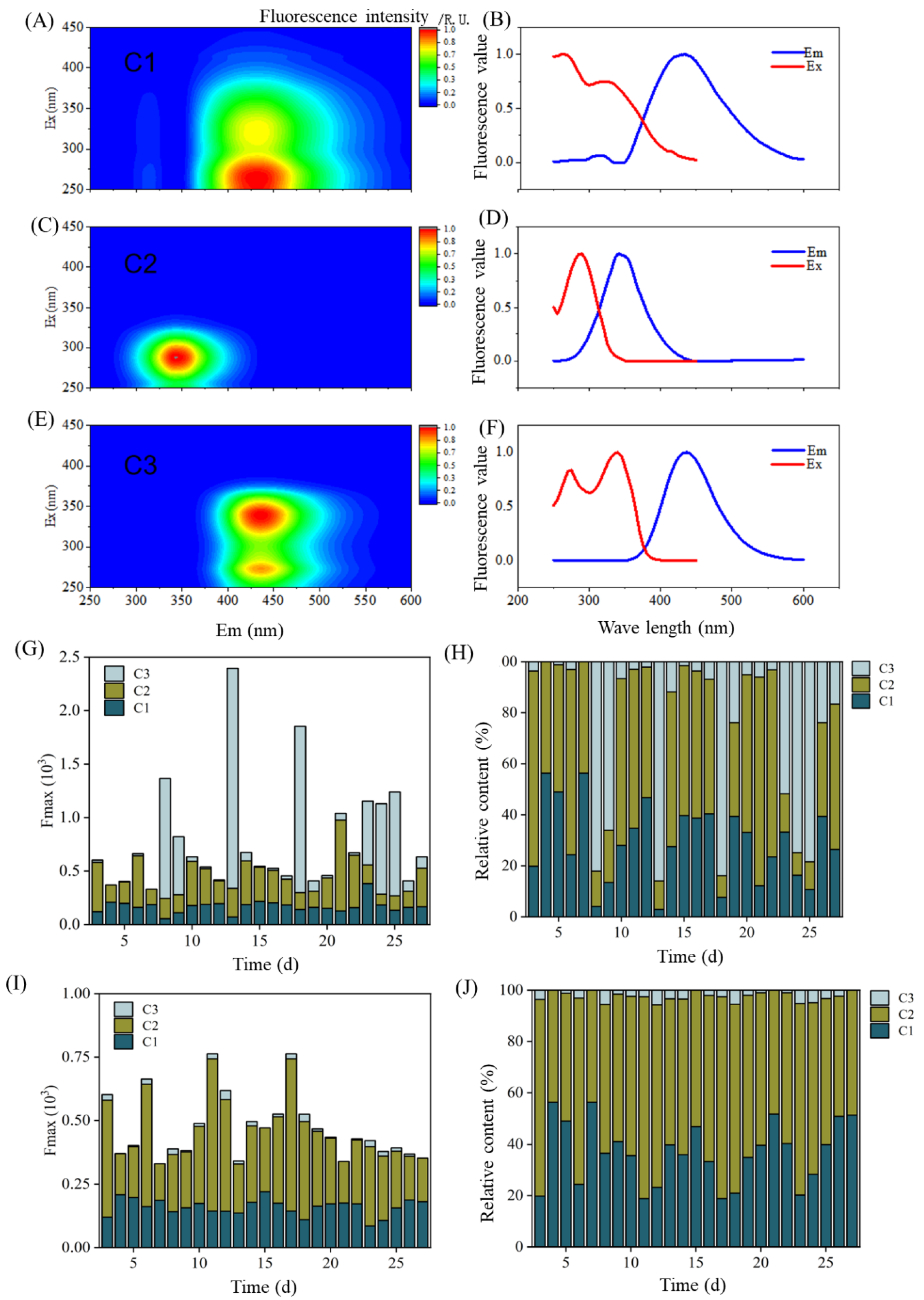
2.3.1. Decay and Composition Change of Plant Decayed Matter

Air dried plant samples (0.2 g) were collected to measure the contents of C, N and P. Nitrogen content in plants (0.2 g) was determined by H2SO4-H2O2 digestion and micro-Kjeldahl determination [13]. The content of phosphorus for the plant samples (0.2 g) was determined by H2SO4-H2O2 digestion, followed by molybdenum-antimony resistance colorimetry [14]. The plant samples were crushed through a 30-mesh screen and 0.02 g samples were used to determine the content of cellulose and lignin [15].
The Olson exponential decay model was used to calculate the decomposition rate of plants.
Mt/M0 = ekt
where t is the experiment time (d); Mt is the dry matter content (g); M0 is the initial dry matter content (d) ;   k is the decomposition rate constant (d−1).

2.3.2. DO and pH in Sediment–Water Interface

DO and pH were measured by plane photopole technology (PO, PO2100) in situ [16]. The PO2100 was used to place the photochemical sensing film between the sediment–water system and the wall of the container. Under the excitation of the light source, the photochemical sensing film converted the measured substance content into optical signals and recorded them with a CMOS camera (Hamamatsu Photonics, Shizuoka, Japan). The change in DO and pH concentrations was visualized through software analysis.

2.3.3. Determination of Organic Matter in Sediment

Air-dried sediment samples (0.2 g) were collected to measure the total organic carbon (TOC) [7]. Light recombinant organic matter (LFOM/HFOM) was quantified based on the previous method [17]. Specifically, the 5 g processed sediment sample was weighed, and 20 mL 1.8 g/mL sodium iodide heavy solution was added. The sample was shaken in the vibrating machine for 1 h (250 rpm/min), centrifuged for 15 min (3500 r/min) and filtered by filter membrane (calcined at 550 °C for 4 h); this was repeated three times. Concentration of active organic matter (AOM) was quantified based on the previous method [18]. Specifically, 0.5 g of the sediment sample was put into a 50 mL plastic centrifuge tube, and 25 mL of 333 mmol/L KMnO4 solution was added. The sample was shocked at 250 r/min for 1 h, and centrifuged at 4000 r/min for 15 min. Then, the supernatant was diluted 250 times with pure water, and absorbance was measured at 565 nm by spectrophotometer (Shimadu, Kyoto, Japan). DOM in sediments was extracted and quantified followed by previous method [19]. An amount of 4 g sediment sample (sifted through 100 mesh) was diluted with 40 mL pure water. The sample was oscillated at a constant temperature for 16 h (20 °C, 220 r/min) and centrifuged at a speed of 4000 r/min for 20 min. Filtration was performed using 0.45 µm microporous membrane (burned at 450 °C for 4 h) for analysis.
Fluorescence spectrometer (Hitachi F-7000) was used for the analysis of dissolved organic matter (DOM). The scanning speed was 12,000 nm/min, the scanning range of the excitation wavelength was 200–500 nm and the step length was 5 nm. The scanning range of emission wavelength is 250–600 nm, and the step length is 1 nm [20]. The ultraviolet absorption spectra of the experiment were measured using an Epoch Microplate Spectrophotometer (BioTek, Charlotte, VT, USA).

2.3.4. Gas Collection and Analysis

CO2 and CH4 concentrations in porewater and overlying water were measured using the headspace equilibration method [21,22]. Briefly, a 10 mL water sample was collected from Rhizon samplers pre-loaded into PVC tubes using a 50 mL polypropylene syringe equipped with three-way stopcocks. An amount of 20 mL ambient air was added to the syringe to create a headspace. Then, the sample syringe was shaken vigorously for 2 min. The equilibrated headspace gas was injected into a pre-evacuated Exetainer® vial (839 W, Labco, High Wycombe, UK) for storage. The flux of CO2 and CH4 across the overlying water—air interface were analyzed using a static microchamber method described by Shi et al. (2018). On dayS 0, 7, 14, 28 and 42, the microchamber was placed onto the water surface in each PVC tube. The gas samples (10 mL) were collected twice using a 25 mL polypropylene syringe, with a 4 h interval before and after. The samples were also injected into a pre-evacuated Exetainer® vial (839 W, Labco, UK) for storage until analysis. CO2 and CH4 concentrations in all vials were analyzed using a gas chromatograph (7890B, Agilent Technologies, Santa Clara, CA, USA). According to the difference in gas concentrations in pore water and overlying water, Fick’s first law was used to calculate the GHG diffusion flux at the SWI [23].
F = DS × ∆C/∆Z = DS × (CpCw)/∆Z
where
F: Gas diffusion flux at the sediment–water interface (μmol/cm2/s),
DS: Effective diffusion coefficient of gas (1/cm2/s),
C: Difference in gas concentration at the sediment–water interface (μmol/cm2),
Z: Gas diffusion distance (cm),
Cp: Gas concentration in sediment pore water (μmol/cm2),
Cw: Gas concentration in overlying water (μmol/cm2).
The calculation of diffusion coefficient DS should take into account the diffusion coefficient of gas in water and the porosity of sediment.
D S = D w   ×   φ 2
where
Dw: Diffusion coefficient of gas in water (cm2/s),
φ : Sediment porosity, φ = 0.88,
Dw: Can be calculated according to the empirical formula related to temperature when the ambient temperature (T) was 0~35 °C [24].
DW-CO2 = 3.17 × 10⁻¹¹T3 + 2.6 × 10⁻⁹T2 + 3.1 × 10⁻⁷T + 9.2 × 10⁻⁶
DW-CH4 = 8.9 × 10⁻¹¹T3 − 1.7 × 10⁻⁹T2 + 3.7 × 10⁻⁷T + 8.8 × 10⁻⁶
where
DW-CO2 and DW-CH4: Diffusion coefficients of CO2 and CH4 in water (cm2/s),
T: Temperature, T = 30 °C.
Fick’s first law was used to calculate the GHG diffusion flux at the water–air interface according to the difference between the concentration of GHG in the sediment and the concentration of GHG in the atmosphere (Liss and Slater 1974).
F = kC/∆Z = Dw (CACw)/∆Z
where
F: Gas diffusion flux at the water–gas interface (μmol/cm2/s),
K: Effective diffusion coefficient of gas (cm2/s),
Dw: Diffusion coefficient of gas in water (cm2/s),
C: Difference in gas concentration at the sediment–water interface (μmol/cm2),
Z: Gas diffusion distance (cm),
CA: Concentration of gases in the atmosphere (μmol/L),
Cw: Gas concentration in overlying water (μmol/L).

2.3.5. Microbial Community Analysis

An amount of 5 g fresh sediments and 500 mL water samples were collected from each system on day 42 for sediment microbial analysis. The water samples were taken and filtered through a 0.22 µm filter membrane. DNA was extracted using E.Z.N.A.® Soil DNA Kit (Omega Bio-tek, Norcross, GA, USA) following the manufacturer’s protocols. Concentration and purity of extracted DNA were determined with TBS-380 and NanoDrop2000, respectively. DNA extract quality was checked on 1% agarose gel. DNA extract was fragmented to an average size of about 400 bp using Covaris M220 (Gene Company Limited, Shanghai, China) for paired-end library construction. The paired-end library was constructed using NEXTflexTM Rapid DNA-Seq (Bioo Scientific, Austin, TX, USA). Adapters containing the full complement of sequencing primer hybridization sites were ligated to the blunt-end of fragments. Paired-end sequencing was performed on Illumina NovaSeq/Hiseq Xten (Illumina Inc., San Diego, CA, USA) at Majorbio Bio-Pharm Technology Co., Ltd. (Shanghai, China) using NovaSeq Reagent Kits/HiSeq X Reagent Kits according to the manufacturer’s instructions (www.illumina.com, accessed on 10 February 2023).
Representative sequences of a non-redundant gene catalog were annotated based on the NCBI NR database using blastp, as implemented in DIAMOND v0.9.19 with an e-value cutoff of 1 × 10⁻⁵ using Diamond (http://www.diamondsearch.org, accessed on 10 February 2023, version 0.8.35) for taxonomic annotations. Cluster of orthologous groups of proteins (COG) annotation for the representative sequences was performed using Diamond (http://www.diamondsearch.org/index.php, accessed on 10 February 2023, version 0.8.35) against eggNOG database (version 4.5.1) with an e-value cutoff of 1 × 10⁻⁵. The KEGG annotation was conducted using Diamond (http://www.diamondsearch.org, accessed on 10 February 2023, version 0.8.35) against the Kyoto Encyclopedia of Genes and Genomes database (http://www.genome.jp, accessed on 10 February 2023, version 94.2) with an e-value cutoff of 1 × 10⁻⁵.

2.4. Statistical Analysis

Correlations between each pair of two variables were analyzed using the Pearson correlation coefficient. The difference in two variables was analyzed by the independent samples t-test at a p < 0.05 level of significance. Statistical analysis was performed using SPSS v 13.0 software.

3. Results and Discussion

3.1. Changes of Organic Matter in Sediment–Water Environment

3.1.1. Decay of Plant Decayed Matter

The decomposition of aquatic plants is mainly caused by microbial degradation. As shown in Figure 1A, the contents of total carbon for the Cattail group were significantly higher (p < 0.01) than that of the Crispus group, suggesting that different aquatic plants possess different contents of carbon. In the first three days of decomposition, the contents of total carbon in the Crispus group and the Cattail group significantly decreased (p < 0.01) from 457.53 ± 29.07 mg/g and 796.39 ± 31.68 mg/g to 347.54 ± 36.46 mg/g and 690.07 ± 32.62 mg/g, respectively. This was mainly due to the decomposition and release of leachable matter (i.e., protein and carbohydrates) at the initial stage [7]. After about a week, the contents of total carbon started to increase gradually, likely because the relative contents of cellulose, lignin and other non-degradable substances increased at the later stage of decomposition.
Similarly, significant decreases in N and P contents were also observed in the Crispus group and the Cattail group during the first week (p < 0.01, Figure 1B,C). For example, the N content decreased from 8.63 ± 0.15 mg/g and 4.33 ± 0.11 mg/g to 3.93 ± 0.07 mg/g and 1.45 ± 0.03 mg/g in the first three days in the Crispus group and Cattail group (Figure 1B), respectively. Different to the contents of C, the Crispus group possessed significantly higher amounts of N and P (p < 0.01) than the Cattail group, suggesting that the contents of key elements might be varied between different aquatic plants.
Crude fibers such as lignin and cellulose are difficult to decompose, which are mostly found in the cell walls of plants. The contents of cellulose in the Crispus group and Cattail group were significantly decreased (p < 0.01) from 184.87 ± 8.99 mg/g and 262.23 ± 22.14 mg/g to 86.98 ± 10.87 mg/g and 197.82 ± 19.34 mg/g in one week, respectively (Figure 1D). At the later stage, the decomposition rates of cellulose slowed down and the cellulose content reached a relatively stable value. In plant cells, lignin is covalently bonded with hemicellulose and coated with cellulose, which can prevent the continuous degradation of plants [25]. Thus, the degradation of lignin is usually a very slow process. It was found that the lignin content remained relatively stable during the entire decomposition process (Figure 1E). Notably, the contents of lignin and cellulose in the Cattail group were significantly higher (p < 0.01) than in the Crispus group (Figure 1D,E).
The dry matter of both plants was significantly decreased before day 20 and remained stable at the later stage (Figure 1F,G). For instance, dry matter residues of the Crispus group and the Cattail group decreased by 27.5% and 17.5% on day 6, respectively; they further decreased by 36.2% and 27.7% at the end of the experiment, respectively. In addition, the plant decomposition rates of the Crispus and Cattail groups gradually decreased during the process, and the decomposition rate of the Crispus group was consistently higher than the Cattail group. This is in line with the higher amount of lignin and cellulose observed in the Cattail group because these two compounds are known to be difficult to degrade. Moreover, the ratio of C/N is another indicator of the decomposition rate of plants [7,26], and a low C/N ratio generally leads to faster decomposition of aquatic plants. In agreement with this hypothesis, the initial C/N of Potamogeton crispus was 53.0, which is much lower than Typha orientalis Presl with 183.9.

3.1.2. Effects of Decomposition of Aquatic Plants on Organic Matter in Sediments

The characteristics of water bodies would be changed due to the decomposition of aquatic plants [27]. Meanwhile, microbial growth is also promoted, and C and H transformation is accelerated, resulting in changes in CO2 and CH4 contents [2,28]. Hence, the characteristics of organic matter in sediments were analyzed during the decomposition of aquatic plants. TOC of the Crispus group and Cattail group increased significantly (p < 0.05) before 7 d, reaching the peak values of 32.42 ± 1.58 mg/g and 31.68 ± 0.96 mg/g, respectively (Figure 2A). The results indicated that the deposition of soluble organic carbon in plants during plant decomposition could lead to TOC accumulation, and the cumulative effect was greater than that of microbial degradation. After the 7th day, TOC contents decreased, probably because of microbial degradation. During degradation, organic matter escaped as methane and carbon dioxide [7,29]. There were no significant differences in TOC content between the two groups.
Due to different densities, organic matter in sediments can be divided into light-fraction organic matter (LFOM) and heavy-fraction organic matter (HFOM) [30]. LFOM and HFOM have different effects on carbon and nitrogen cycling. LFOM has a higher turnover rate, C/H ratio and lower relative density, and more than 50% of microbial and enzyme activities are related to LFOM [30,31]. The contents of LFOM in the sediments of the two groups increased with plant decomposition (Figure 2B), possibly because the fresh organic matter was generated by plant decomposition. It can be seen from Figure 2B that the content of HFOM ranged from 19.03 ± 1.70 to 27.18 ± 0.69 mg/g accounting for more than 80% of the total organic matter. On the 7th day of plant decomposition, the average contents of HFOM for the Crispus group and Cattail group reached peak values of 32.42 ± 1.58 mg/g and 31.68 ± 0.96 mg/g, respectively (Figure 2C). After the 7th day, HFOM contents of the two groups decreased.
The average contents of active organic matter (AOM) in the Crispus group and Cattail group increased significantly (p < 0.05), and the values reached 1840.63 ± 499.92 mg/kg and 1666.43 ± 350.86 mg/kg in 7 d, respectively (Figure 2D). It might be due to the migration of soluble organic carbon from the overlying water to the sediment interstitial water; thus, this increased the contents of AOM in the interstitial water [9]. The content of AOM showed a decreasing trend after the 7th day of the experiment, which is due to AOM being easily degraded by microorganisms. After 14 days of the experiment, the contents of AOM in the two groups were increased, indicating that AOM in sediment was affected by plant decomposition and sedimentation [7].
Three fluorescent components of DOM were further verified by the three-dimensional fluorescence spectral matrix in sediments during decomposition of two aquatic plants (Figure 3). C1 has the main excitation and emission peaks at Ex/Em = 265/433 nm. C2 has an excitation and emission peak at Ex/Em = 285/341 nm. At Ex/Em = 340/436 nm, C3 has the main excitation and emission peaks. C1 was classified as a humic acid component because the Ex peak of C1 was located at 265 nm in the short-wave ultraviolet region [7,32]. C2 could be classified as the tryptophan component of proteoid [32], which was mainly produced by biological activities in water, and could well reflect the autogenic process of water (Figure 3C,D). C3 was a component of fulvic acid in the region of long-wave ultraviolet [33]. The intensity of C1 and C3 components in the secondary peak was obviously weaker than that of the main peak (Figure 3A,B,E,F), which is a comprehensive product of terrestrial input, water microbial activity and photochemical oxidation.
The total fluorescence contents of the Crispus group were higher than those of the Cattail group (Figure 3G–J). These results indicated that more DOM was released during the decomposition of the Crispus group. It could be seen that in the process of plant decomposition, the DOM was mainly composed of C2, followed by C1 and C3 (Figure 3G–J). For instance, in the Crispus group, relative percentages of C1 ranged from 2.91% to 56.35%, and the average relative content was 28.95%. C2 and C3 with average relative content were 45.24% and 25.81%, respectively.

3.2. DO and pH in the Sediment–Water Interface

The content of DO can reflect the water pollution. Figure 4A,B showed a two-dimensional diagram of DO at the sediment–water interface. The concentration of DO in the Crispus group was significantly higher (p < 0.05) than that of the Cattail group (Figure 4A,B). This result indicated that Potamogeton crispus had a greater effect on the consumption of DO than that of Typha orientalis Presl during the decomposition process of submerged plants. Moreover, similar trends of DO were observed in the two groups at the sediment–water interface during the process of plant decomposition. In the first week of the experiment, DO concentration dropped rapidly because soluble substances were released from plants into the sediment–water interface and oxygen was consumed by aerobic microorganisms in the initial stage. Afterwards, the concentration of DO was increased slowly from 7 to 42 d. The decomposition rates were reduced because activities of aerobic enzymes decreased under the anoxic environment, and oxygen from the atmosphere would continuously enter the sediment–water system [34]. Additionally, oxygen might be also produced by photosynthetic bacteria to supplement the DO in the water environment with the process of plant decomposition [31]. Hence, multiple factors, including reduction of oxygen consumption and increase of oxygen input, might play key roles in the increase of DO in the sediment–water interface.
Similar changes in pH were found in the two groups during the decomposition (Figure 4C,D). The pH in the Crispus group was significantly higher (p < 0.05) than that of the Cattail group (Figure 4C,D). More organic acids were produced in the early stage of plant decomposition, resulting in the decrease of pH from 0 to 7 d. The pH increased slowly after day 7, indicating the decreased decomposition rate. The average contents of active organic matter (AOM) in the Crispus group and Cattail group were increased significantly (p < 0.05), reaching 1840.6 ± 499.9 mg/kg and 1666.4 ± 350.9 mg/kg on day 7, respectively (Figure 2D).

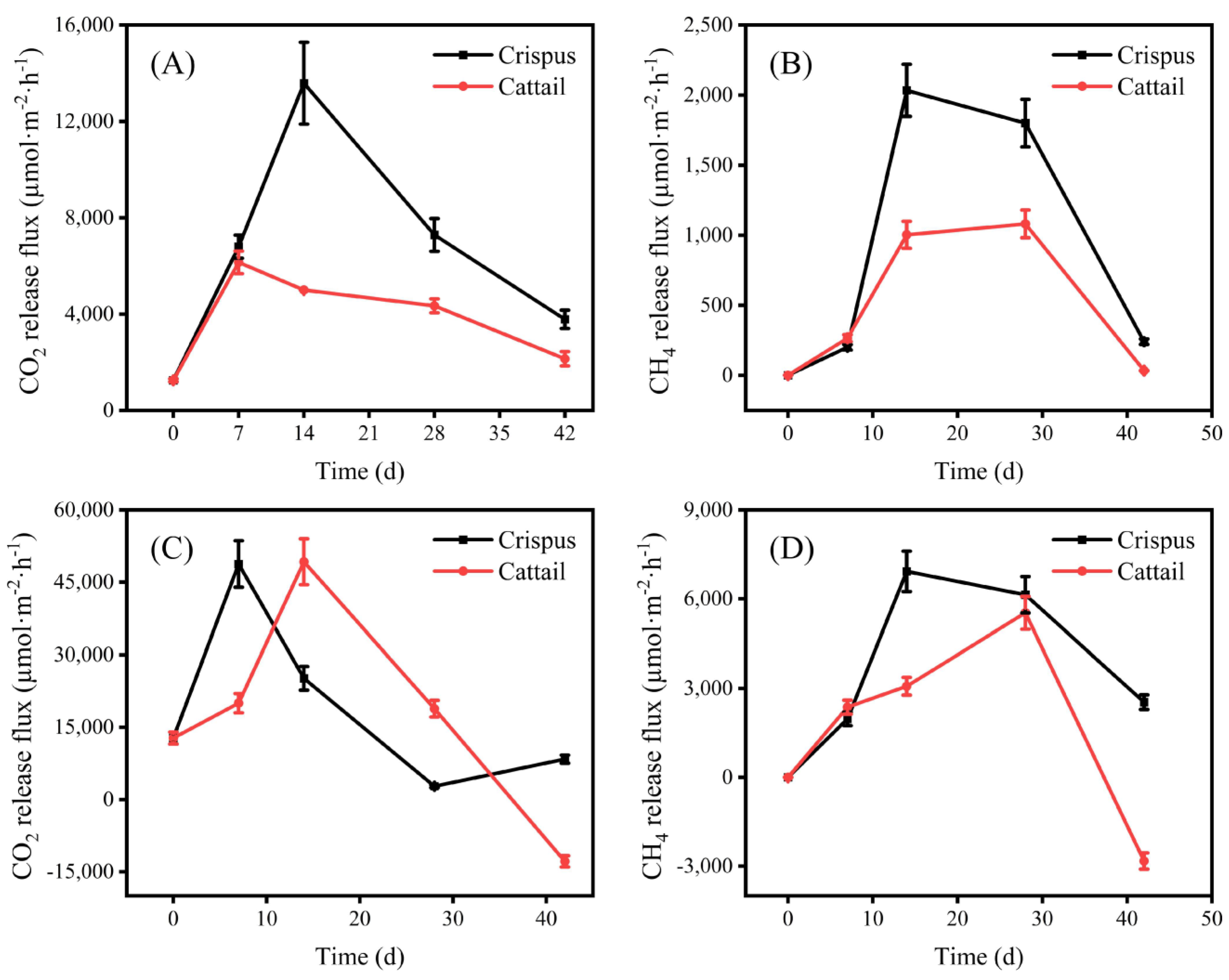
3.3. Changes of CO2 and CH4 Flux

The decomposition of aquatic plants released a large number of organic matters into the water, which can be decomposed by microorganisms to produce CH4 and CO2 [7]. Concentrations of GHG (i.e., CH4 and CO2) in overlying water and sediment were measured, and their flux at the water–gas interface and sediment–water interface were calculated (Figure 5). Changes in CO2 flux released from overlying water to the atmosphere during plant decomposition were shown in Figure 5A. During the early decomposition, CO2 emission flux of the Crispus group increased significantly (p < 0.05) before day 14, reaching the peak value of 13,587.9 µmol/m2/h, and then reduced immediately, which may be related to the decomposition process of Potamogeton crispus. Before the 14th day, the decomposition rate of Potamogeton crispus was faster, resulting in the decomposition of a large amount of organic matter, which promoted the release of CO2 [35]. In addition, the emission flux of CO2 in the Crispus group was significantly higher (p < 0.05) than that of the Cattail group after 7 days of decomposition process (Figure 5A). The cumulative emissions of CO2 released from overlying water to the atmosphere were significantly (p < 0.05) greater in the Crispus group than in the Cattail group through the study period, with 60,875.29 µmol and 33,104.07 µmol, respectively.
The change of CO2 flux released from sediment to overlying water during plant decomposition was shown in Figure 5B. The emission flux of CO2 also increased significantly (p < 0.05) in the two groups during the early decomposition. The emission flux of CO2 in the Crispus group and the Cattail group reached the maximum values on the day 7 (48,777.4 µmol/m2/h) and day 14 (49,227.8 µmol/m2/h), respectively (Figure 5B). However, CO2 flux in sediments continued to decrease during the plant decomposition from day 14 to day 42. This might be due to CO2 is converted to CH4 by anaerobic microorganisms [2,36]. The diffusion flux of CO2 at the sediment–water interface was higher than that at the water–gas interface, indicating that mineralization of organic carbon in the sediment was one of the main sources of CO2. This result also indicated that Potamogeton crispus had a greater effect on CO2 emission flux than Typha orientalis Presl during the decomposition process. The cumulative emissions of CO2 released from sediment to overlying water were significantly (p < 0.05) lower in the Crispus group than in the Cattail group through the study period, with 140,837.7 µmol and 165,020.2 µmol, respectively.
The variation of CH4 released into the atmosphere from overlying water during plant decomposition was shown in Figure 5C. The diffusion flux of CH4 did not change significantly at the early stage of decomposition (day 0 to day 7), but significantly increased (p < 0.05) during day 7 to day 14, and decreased at the late stage of decomposition. In addition, the emission flux of CH4 in the Crispus group was significantly higher (p < 0.05) than that of the Cattail group after 7 days of decomposition process (Figure 5C). The result indicated that the flux of CH4 emitted from overlying water during plant decomposition was the “source” of atmospheric GHGs [2]. The cumulative emissions of CH4 released from overlying water to the atmosphere were significantly (p < 0.05) greater in the Crispus group than in the Cattail group through the study period, with 9355.49 µmol and 5232.24 µmol, respectively.
Changes of CH4 released from sediments to overlying water during plant decomposition was shown in Figure 5D. At the initial stage of plant decomposition, the flux of CH4 increased significantly (p < 0.05), which was different from the trend of CH4 released from overlying water to the atmosphere, possibly due to the oxidation of CH4 released from sediment during the emission process. Afterwards, the flux decreased continuously after reaching the peak value in the Crispus and Cattail groups, which might be due to the rapid decomposition of soluble organic matter in the early stage of plant decomposition, and the significant reduction of DO, forming suitable conditions for generation of CH4 [7]. In addition, the emission flux of CH4 in the Crispus group were significantly higher (p < 0.05) than that of the Cattail group after 7 days of decomposition process (Figure 5D). For instance, the emission flux of CH4 in the Crispus and Cattail groups were 6926.2 µmol/m2/h and 2455.3 µmol/m2/h at day 14, respectively, which may be related to the higher content of LFOM in sediments of Crispus group (Figure 2B), which provides more substrates for Methanogen [37]. The cumulative emissions of CH4 released from sediment to overlying water were significantly (p < 0.05) greater in the Crispus group than in the Cattail group through the study period, with 35,827.72 µmol and 20,057.55 µmol, respectively.
Differentially function gene associated with production of CO2 and CH4 between the Crispus and Cattail groups were compared based on genome-wide DNA sequencing (Figure 6). Abundances of genes related to CO2 metabolism were decreased during day 7 to day 42 in overlying water. It should be noted that decrease of abundances of these genes might lose of cell function, thus resulting in a decreased CO2 emission flux. That is why the CO2 flux continued to decrease during the plant decomposition from day 14 to day 42. In addition, abundances of these genes in the overlying water of the Cattail group were higher than that of the Crispus group on the day 7. However, these genes in the overlying water, showed that the Crispus group have higher abundance compared with the Cattail group after 7 days of decomposition process (Figure 6), which might be contributing to the high emission flux of CO2 in the Crispus group. About genes related to CH4 metabolism, abundances were increased during day 7 to day 42 in overlying water. Consistent with results of genes related to CO2 metabolism, abundances of these genes in the overlying water of the Crispus group were higher than those of the Cattail group on day 42 (Figure 6). This result further supports the finding that the emission flux of CH4 in the Crispus group was significantly higher (p < 0.05) than that of the Cattail group after 7 days of the decomposition process.
To investigate the mechanism of CO2 and CH4 release from overlying sediment–water by plant decomposition, the correlation analysis among the contents of CO2, CH4, TOC, AOM, LFOM and HFOM was carried out (Table 1). There was a significant negative correlation between CH4 release and TOC content (R = −0.335, p < 0.05), and a significant positive correlation between CH4 release and LFOM content (R = 0.363, p < 0.05). Additionally, a significant positive correlation was observed between CO2 and LFOM (R = 0.386, p < 0.05), indicating that CO2 and CH4 were the final products of organic matter mineralization, and CO2 and CH4 were released at the same time.

4. Conclusions

The contents of C, lignin and cellulose in the Potamogeton crispus were significantly lower than those of the Typha orientalis Presl, except for N and P. The contents of LFOM in the sediments of the two groups were increased with plant decomposition. During the early decomposition, CO2 emission flux were increased significantly in the two groups. The diffusion flux of CH4 did not change significantly at the early stage of decomposition (day 0 to day 7), but was significantly increased during day 7 to day 14, and decreased at the late stage of decomposition. Abundances of genes related to CO2 and CH4 metabolism in the overlying water of the Crispus group were higher than those of the Cattail group on day 42. The decomposition of aquatic plants, in contrast, increased the LFOM content in the sediment, providing sufficient substrate for the production of CO2 and CH4; the relative abundance of anaerobic microorganisms also increased. Under this dual action, the release of CO2 and CH4 was promoted. It is worth noting that the release flux of CH4 and CO2 in the indoor simulation experiment are much larger than those detected in the field, so it is necessary to further combine the field experiment to clarify the relevant mechanism.

Author Contributions

J.X.: Investigation, Writing—Original Draft, Funding acquisition. Y.G.: Visualization, Investigation. X.X. and T.C.: Reviewing, Editing. L.T.: Data curation. C.Z.: Interpreting data. J.C.: Resources, Project administration. T.H.: Reviewing, Supervision, Conceptualization, Methodology, Project administration. All authors have read and agreed to the published version of the manuscript.

Funding

This work was financially supported by the Natural Science Foundation of Jiangsu Province (BK20200816), the Key University Science Research Project of Jiangsu Province (20KJB610009), the Special Fund of Chinese Central Government for Basic Scientific Research Operations in commonweal Research Institute (GYZX220102), and the Xinjiang Science and Technology Support Project Plan (2022E02026).

Data Availability Statement

The datasets used and/or analyzed during the current study are available from the corresponding author on reasonable request.

Conflicts of Interest

The authors declare no conflict of interest.

References

  1. Bongaarts, J. Intergovernmental panel on climate change special report on global warming of 1.5 °C Switzerland: IPCC. Popul. Dev. Rev. 2019, 45, 251–252. [Google Scholar] [CrossRef] [Green Version]
  2. Wang, G.Q.; Xia, X.H.; Liu, S.D.; Zhang, L.; Zhang, S.B.; Wang, J.F.; Xi, N.N.; Zhang, Q.R. Intense methane ebullition from urban inland waters and its significant contribution to greenhouse gas emissions. Water Res. 2021, 189, 116654. [Google Scholar] [CrossRef] [PubMed]
  3. Kirschke, S.; Bousquet, P.; Ciais, P.; Saunois, M.; Canadell, J.G.; Dlugokencky, E.J.; Bergamaschi, P.; Bergmann, D.; Blake, D.R.; Bruhwiler, L. Three decades of global methane sources and sinks. Nat. Geosci. 2013, 6, 813–823. [Google Scholar] [CrossRef] [Green Version]
  4. Saunois, M.; Bousquet, P.; Poulter, B.; Peregon, A.; Ciais, P.; Canadell, J.; Dlugokencky, E.; Etiope, G.; Bastviken, D.; Houweling, S. The global methane budget 2000–2012. Earth Syst. Sci. Data 2016, 8, 697–751. [Google Scholar] [CrossRef] [Green Version]
  5. Marano, A.V.; Pires-Zottarelli, C.L.A.; Barrera, M.D.; Steciow, M.M.; Gleason, F.H. Diversity, role in decomposition, and succession of zoosporic fungi and straminipiles on submerged decaying leaves in a woodland stream. Hydrobiologia 2011, 659, 93–109. [Google Scholar] [CrossRef]
  6. Serna, A.; Richards, J.H.; Scinto, L.J. Plant decomposition in wetlands: Effects of hydrologic variation in a re-created everglades. J. Environ. Qual. 2013, 42, 562–572. [Google Scholar] [CrossRef]
  7. Luo, P.; Tong, X.; Liu, F.; Huang, M.; Xu, J.; Xiao, R.; Wu, J. Nutrients release and greenhouse gas emission during decomposition of Myriophyllum aquaticum in a sediment-water system. Environ. Pollut. 2020, 260, 114015. [Google Scholar] [CrossRef]
  8. Velthuis, M.; Kosten, S.; Aben, R.; Kazanjian, G.; Hilt, S.; Peeters, E.T.H.M.; Van Donk, E.; Bakker, E.S. Warming enhances sedimentation and decomposition of organic carbon in shallow macrophyte-dominated systems with zero net effect on carbon burial. Glob. Chang. Biol. 2018, 24, 5231–5242. [Google Scholar] [CrossRef] [PubMed] [Green Version]
  9. Bartosiewicz, M.; Maranger, R.; Przytulska, A.; Laurion, I. Effects of phytoplankton blooms on fluxes and emissions of greenhouse gases in a eutrophic lake. Water Res. 2021, 196, 116985. [Google Scholar] [CrossRef] [PubMed]
  10. Wang, M.; Hao, T.; Deng, X.; Wang, Z.; Cai, Z.; Li, Z. Effects of sediment-borne nutrient and litter quality on macrophyte decomposition and nutrient release. Hydrobiologia 2017, 787, 205–215. [Google Scholar] [CrossRef]
  11. Li, X.; Cui, B.; Yang, Q.; Lan, Y.; Wang, T.; Han, Z. Effects of plant species on macrophyte decomposition under three nutrient conditions in a eutrophic shallow lake, North China. Ecol. Model. 2013, 252, 121–128. [Google Scholar] [CrossRef]
  12. Suzuki, M.S.; Fonseca, M.N.; Esteves, B.S.; Chagas, G.G. Decomposition of Egeria densa Planchon (Hydrocharitaceae) in a well oxygenated tropical aquatic ecosystem. J. Limnol. 2015, 74, 278–285. [Google Scholar] [CrossRef] [Green Version]
  13. Yu, M.F.; Tao, Y.; Liu, W.; Xing, W.; Liu, G.; Wang, L.; Ma, L. C, N, and P stoichiometry and their interaction with different plant communities and soils in subtropical riparian wetlands. Environ. Sci. Pollut. Res. 2020, 27, 1024–1034. [Google Scholar] [CrossRef] [PubMed]
  14. Guo, L.L.; Yu, Z.H.; Li, Y.S.; Xie, Z.H.; Wang, G.H.; Liu, X.B.; Liu, J.J.; Liu, J.D.; Jin, J. Plant phosphorus acquisition links to phosphorus transformation in the rhizospheres of soybean and rice grown under CO2 and temperature co-elevation. Sci. Total Environ. 2022, 826, 153558. [Google Scholar] [CrossRef]
  15. Xu, F.; Yu, J.; Tesso, T.; Dowell, F.; Wang, D. Qualitative and quantitative analysis of lignocellulosic biomass using infrared techniques: A mini-review. Appl. Energy 2013, 104, 801–809. [Google Scholar] [CrossRef] [Green Version]
  16. Glud, R.N.; Ramsing, N.B.; Gundersen, J.K.; Klimant, I. Planar optrodes: A new tool for fine scale measurements of two-dimensional O2 distribution in benthic communities. Mar. Ecol. Prog. Ser. 1996, 140, 217–226. [Google Scholar] [CrossRef]
  17. Janzen, H.H.; Campbell, C.A.; Brandt, S.A.; Lafond, G.P.; Townley-Smith, L. Light-fraction organic matter in soils from long-term crop rotations. Soil Sci. Soc. Am. J. 1992, 56, 1799–1806. [Google Scholar] [CrossRef] [Green Version]
  18. Gao, H.J.; Peng, C.; Zhang, X.Z.; Li, Q.; Zhu, P. Effects of Long-term Fertilization on Maize Yield, Active Organic Matter and pH Value of Black Soil. J. Maize Sci. 2014, 22, 126–131. [Google Scholar]
  19. Strobel, B.W.; Hansen, H.C.B.; Borggaard, O.K.; Andersen, M.K.; Raulund-Rasmussen, K. Composition and reactivity of DOC in forest floor soil solutions in relation to tree species and soil type. Biogeochemistry 2001, 56, 1–26. [Google Scholar] [CrossRef]
  20. Hudson, N.; Baker, A.; Reynolds, D.M. Fluorescence analysis of dissolved organic matter in natural, waste and polluted waters—A review. River Res. Appl. 2007, 23, 631–649. [Google Scholar] [CrossRef]
  21. Shi, W.Q.; Chen, Q.W.; Zhang, J.Y.; Liu, D.S.; Yi, Q.T.; Chen, Y.C.; Ma, H.H.; Hu, L.M. Nitrous oxide emissions from cascade hydropower reservoirs in the upper Mekong River. Water Res. 2020, 173, 115582. [Google Scholar] [CrossRef] [PubMed]
  22. Wang, S.L.; Liu, C.Q.; Yeager, K.M.; Wan, G.J.; Li, J.; Tao, F.X.; Lue, Y.C.; Liu, F.; Fan, C.X. The spatial distribution and emission of nitrous oxide (N2O) in a large eutrophic lake in eastern China: Anthropogenic effects. Sci. Total Environ. 2009, 407, 3330–3337. [Google Scholar] [CrossRef] [PubMed]
  23. Trfmbly, A.; Varflvy, L.; Roehm, C.; Garneau, M. Green House Gas Emisions—Fluxes and Proceses; Springer: Berlin/Heidelberg, Germany, 2005. [Google Scholar]
  24. Banks, L.K.; Frost, P.C. Biomass loss and nutrient release from decomposing aquatic macrophytes: Effects of detrital mixing. Aquat. Sci. 2017, 79, 881–890. [Google Scholar] [CrossRef]
  25. Yu, Z.J.; Deng, H.G.; Wang, D.Q.; Ye, M.W.; Tan, Y.J.; Li, Y.J.; Chen, Z.L.; Xu, S.Y. Nitrous oxide emissions in the Shanghai river network: Implications for the effects of urban sewage and IPCC methodology. Glob. Chang. Biol. 2013, 19, 2999–3010. [Google Scholar] [CrossRef]
  26. Longhi, D.; Bartoli, M.; Viaroli, P. Decomposition of four macrophytes in wetland sediments: Organic matter and nutrient decay and associated benthic processes. Aquat. Bot. 2008, 89, 303–310. [Google Scholar] [CrossRef]
  27. Li, C.H.; Wang, B.; Ye, C.; Ba, Y.X. The release of nitrogen and phosphorus during the decomposition process of submerged macrophyte (Hydrilla verticillata Royle) with different biomass levels. Ecol. Eng. 2014, 70, 268–274. [Google Scholar] [CrossRef]
  28. Wang, L.; Liu, Q.; Hu, C.; Liang, R.; Qiu, J.; Wang, Y. Phosphorus release during decomposition of the submerged macrophyte Potamogeton crispus. Limnology 2018, 19, 355–366. [Google Scholar] [CrossRef] [Green Version]
  29. Hirota, M.; Tang, Y.; Hu, Q.; Hirata, S.; Kato, T.; Mo, W.; Cao, G.; Mariko, S. Carbon dioxide dynamics and controls in a deep-water wetland on the Qinghai-Tibetan Plateau. Ecosystems 2006, 9, 673–688. [Google Scholar] [CrossRef]
  30. Whalena, J.K.; Bottomley, P.J.; Myrold, D.D. Carbon and nitrogen mineralization from light- and heavyfraction additions to soil. Soil Biol. Biochem. 2000, 32, 1345–1352. [Google Scholar] [CrossRef]
  31. Zhao, B.; Xing, P.; Wu, Q.L. Microbes participated in macrophyte leaf litters decomposition in freshwater habitat. FEMS Microbiol. Ecol. 2017, 93, fix108. [Google Scholar] [CrossRef] [Green Version]
  32. Qu, F.; Liang, H.; Wang, Z.; Wang, H.; Yu, H.; Li, G. Ultrafiltration membrane fouling by extracellular organic matters (EOM) of Microcystis aeruginosa in stationary phase: Influences of interfacial characteristics of foulants and fouling mechanisms. Water Res. 2012, 46, 1490–1500. [Google Scholar] [CrossRef] [PubMed]
  33. Fellman, J.B.; Hood, E.; Spencer, R.G.M. Fluorescence spectroscopy opens new windows into dissolved organic matter dynamics in freshwater ecosystems: A review. Limnol. Oceanogr. 2010, 55, 2452–2462. [Google Scholar] [CrossRef]
  34. Cornut, J.; Clivot, H.; Chauvet, E.; Elger, A.; Pagnout, C.; Guerold, F. Effect of acidification on leaf litter decomposition in benthic and hyporheic zones of woodland streams. Water Res. 2012, 46, 6430–6444. [Google Scholar] [CrossRef] [Green Version]
  35. Schrier-Uijl, A.P.; Veraart, A.J.; Leffelaar, P.A.; Berendse, F.; Veenendaal, E. Release of CO2 and CH4 from lakes and drainage ditches in temperate wetlands. Biogeochemistry 2011, 102, 265–279. [Google Scholar] [CrossRef] [Green Version]
  36. Zhang, M.; Xiao, Q.; Zhang, Z.; Gao, Y.; Zhao, J.; Pu, Y.; Wang, W.; Xiao, W.; Liu, S.; Lee, X. Methane flux dynamics in a submerged aquatic vegetation zone in a subtropical lake. Sci. Total Environ. 2019, 672, 400–409. [Google Scholar] [CrossRef] [PubMed]
  37. Li, B.; Tao, Y.; Mao, Z.D.; Gu, Q.J.; Han, Y.X.; Hu, B.L.; Wang, H.W.; Lai, A.X.; Xing, P.; Wu, Q.L.L. Iron oxides act as an alternative electron acceptor for aerobic methanotrophs in anoxic lake sediments. Water Res. 2023, 234, 119833. [Google Scholar] [CrossRef]
Figure 1. Composition changes of plant decayed matter in a sediment–water environment. Contents of total carbon (A), N (B), P (C), cellulose (D) and lignin (E) in the Crispus group and Cattail group; Residual rates of dry matter (F) and decomposition rates of Plant (G) in the Crispus group and Cattail group. Values given are the average ± SD of three replicate determinations.
Water 15 02863 g001
Figure 2. Variation characteristics of organic matter in sediments from the Crispus group and Cattail group. Changes of TOC (A), LFOM (B), HFOM (C) and AOM (D) in sediments. Values given are the average ± SD of three replicate determinations.
Water 15 02863 g002
Figure 3. Fluorescent components of DOM in the Crispus group and Cattail group. Fluorescence spectra of C1 (A) and corresponding excitation–emission loads (B); Fluorescence spectra of C2 (C) and corresponding excitation–emission loads (D); Fluorescence spectra of C3 (E) and corresponding excitation–emission loads (F); Fmax values (G) and relative content distribution (H) of fluorescent components in the Crispus group; Fmax values (I) and relative content distribution (J) of fluorescent components in the Cangbo group (From left to right in the order of 0–2, 2–4, 4–6, 6–8, 8–10 cm depth sediments).
Water 15 02863 g003
Figure 4. Changes of DO and pH in the sediment–water interface. The concentrations of DO in the Crispus group (A) and Cattail group (B); Changes of pH in the Crispus group (C) and Cattail group (D).
Water 15 02863 g004
Figure 5. Effects of the decomposition of aquatic plants on CO2 and CH4 release in sediment–water systems. (A) Variation of CO2 emission flux at the water–air interface; (B) Variation of CO2 emission flux at the sediment–water interface; (C) Variation of CH4 emission flux at the water–air interface; (D) Variation of CH4 emission flux at the sediment–water interface. Values given are the average ± SD of three replicate determinations.
Water 15 02863 g005
Figure 6. Abundances of function genes associated with production of CO2 and CH4.
Water 15 02863 g006
Table 1. Correlation coefficients between CO2 and CH4 contents and components of organic matter in sediments (*, p < 0.05; **, p < 0.01).
TOCAOMLFOMHFOMCH4CO2
CH4−0.335 *0.1360.363 **−0.19110.825 **
CO2−0.1330.0350.286 *−0.0130.825 **1
Disclaimer/Publisher’s Note: The statements, opinions and data contained in all publications are solely those of the individual author(s) and contributor(s) and not of MDPI and/or the editor(s). MDPI and/or the editor(s) disclaim responsibility for any injury to people or property resulting from any ideas, methods, instructions or products referred to in the content.

