Longitudinal Mixing in Flows with Submerged Rigid Aquatic Canopies

Abstract

The presence of dense submerged vegetation alters mixing characteristics in open channel flows as they cause differential velocities inside and above canopies. The prediction models for longitudinal mixing in the presence of submerged canopies often use the drag coefficient to represent the canopy, which limits the usability of the models when the canopy properties are not fully understood. Here, attempts were made to present a methodology which can be used for deriving the coefficient of longitudinal dispersion in the presence of submerged vegetation based on velocity measurements, using a mixing length approach to model turbulence. An experimental study was conducted in a large-scale laboratory facility to investigate the longitudinal dispersion characteristics in open channel flow with submerged aquatic vegetation canopies. Detailed velocity and solute tracer measurements were undertaken for a representative range of flow velocities. The velocity measurements were used for deriving turbulent shear stress, mixing length, and diffusivity using established theoretical and empirical relationships to derive the longitudinal dispersion. The longitudinal dispersion measured in two locations in the water column for the two canopy submergences was discussed based on the amount of vertical mixing and differential advection. The canopy with a smaller stem length (i.e., higher submergence ratio) has a higher vertical diffusivity, resulting in increased vertical mixing in the water column. The canopy with the higher stem length (i.e., lower submergence ratio) consists of minimal vertical diffusivity, causing the longitudinal dispersion measured above the canopy to be significantly high, even though the longitudinal dispersion measured inside the canopy is much lower. The mathematical model which was adapted for calculating the coefficient of longitudinal dispersion and the tracer results show good agreement, indicating that the N-zone model can accurately predict the longitudinal dispersion in submerged aquatic canopies when used with the presented methodology.

1. Introduction

Concerns about surface water pollution generate an increased demand for predicting pollution levels in both inland and coastal waters. Understanding how different hydrodynamic conditions affect the fate and pathways of pollutants once they enter a waterbody is crucial for preventing devastating environmental hazards related to water pollution. Often, aquatic vegetation is kept unremoved from the waterways due to the ecosystem services they provide [1], such as improving the water quality [2,3,4,5], reducing turbidity [6], resuspension of nutrients [3,7,8], providing food and shelter for aquatic fauna [3,9,10,11,12], and reducing erosion [3,9,13,14,15]. However, the presence of submerged vegetation in a conveyance channel will alter the mixing of soluble pollutants by introducing a velocity shear at the top of the canopy [16,17,18]. Therefore, studying pollution transport processes in the presence of submerged aquatic vegetation helps with maximising its ecosystem services while reducing the adversity of pollution transport, making it a widely studied topic. Most of these studies on aquatic vegetation parameterize the effects of vegetation using a drag coefficient that depends on the canopy density, flow velocity, and the diameter and morphology of the individual canopy elements [19], thus requiring a comprehensive survey of the channel to determine a representative value for the drag coefficient because aquatic canopies exhibit a wide range of geometries [20].

This paper presents the findings of an experimental study comprising two canopy heights of submerged vegetation, where the velocity measurements are correlated with longitudinal dispersion properties of vegetated open channel flow using established numerical relationships to calculate the coefficient of longitudinal dispersion. A mixing length approach is used for modelling the turbulent shear stress, and the effect of canopy submergence on longitudinal mixing is also discussed based on corresponding velocity profiles.

2. Previous Work

2.1. Flow Velocity in the Presence of Submerged Vegetation

In a wide channel with a bare bed (no effect due to side walls or vegetation), the streamwise velocity profile has a logarithmic shape [21]. If an open channel comprises a submerged sparse canopy where the canopy drag is smaller than the bed drag, the hydrodynamics will not deviate significantly from the open channel conditions, while the canopy contributes to increased bed roughness [19]. Dense aquatic canopies are a source of drag, and the presence of a dense submerged canopy results in a decrease in the flow velocity with distance into the canopy from the top, while increasing the flow velocity above the canopy [14,18,22]. A typical velocity profile in the presence of a dense submerged canopy is shown in Figure 1a. The presence of submerged vegetation also results in a vertical discontinuity of drag [23], resulting in an increase in velocity shear and turbulence intensity at the top of the canopy [11,18]. These processes create instability at the top of the canopy, developing discrete Kelvin-Helmoltz vortices [16] of elliptical shape, as shown in Figure 1b. These vortices are predominantly expressed when the canopy becomes flexible, resulting in a wavy motion in the upper part of the flexible canopies [24].

2.2. Longitudinal Dispersion in the Presence of Submerged Vegetation

The rate of mass transport $\left(\dot{M}\right)$ per unit width in the streamwise direction of a channel is given by Equation (1) [25] in the context of a depth averaged model,

$$\dot{M}=-hD\frac{\partial \overline{C}}{\partial x}$$

(1)

where $h$ is the depth, and the area per unit width of flow, $D$ is called the longitudinal dispersion coefficient which is a bulk transport coefficient representing the diffusive property of the velocity distribution of the flow and $\overline{C}$ is the depth average of the mean concentration.

$D$ is a property of the flow. For example, the velocity profile is logarithmic in wide channels without vegetation, and hence, the coefficient of longitudinal dispersion ($D$) can be expressed by Equation (2) [26],

$$D=5.93 h{u}_{*}$$

(2)

where $u_{*}$ is the friction velocity. The friction velocity is defined in Equation (3),

$$u_{*}=\sqrt{\frac{{\tau }_0}{\rho }}$$

(3)

where ${\tau }_0$ is the shear stress at the channel bed and $\rho$ is the density of the fluid.

Equation (2) can also be used for quantifying longitudinal dispersion in open channels with sparse vegetation if the canopy is sparse enough to maintain the logarithmic shape of the velocity profile. However, $u_{*}$ should be re-evaluated to include the roughness component of the canopy. When the canopy becomes dense, it modifies the velocity profile and the fate and transport of solutes, due to its considerable impact on flow dynamics [18,27]. In such situations, the mixing in the region above the canopy is dominated by large-scale shear dispersion [28]. The flow inside the submerged aquatic canopy can be divided into two regions: (1) a ‘vertical exchange zone’ consisting of Kelvin-Helmoltz vortices [16] in the upper part of the canopy where the rapid vertical turbulent exchange takes place [18], and (2) a ‘longitudinal exchange zone’ in the lower section of the canopy where mixing is dominated by longitudinal advection [17]. The vertical exchange zone created by the vortices penetrates only to a limited distance into the canopy [29] as the shear, which feeds energy to the vortices, is balanced by canopy dissipation [30]. The extent to which the vertical mixing layer grows increases with the depth of submergence and (generally) decreases when the canopy becomes dense or flexible [17]. These complex flow conditions in the presence of submerged canopies can make it challenging to measure longitudinal dispersion. For example, the routing method [31] was unsuccessful when evaluating the coefficient of longitudinal dispersion due to the delay in solute transport inside the canopy and the lack of cross-sectional mixing [32]. On the other hand, the moment area method [26,33] has been adopted for evaluating the coefficient of longitudinal dispersion in vegetated open channel flows [28,34,35].

When a drop of solute is added to a moving water body, it keeps mixing as it moves downstream with the water flow. The concentration time series created by the drop of solute can be measured experimentally using several monitoring stations along the flow. The temporal variance in the measured concentration time series increases along the flow. According to the moment area method, the rate of change in the temporal variance along the flow is used for calculating the longitudinal dispersion coefficient as shown in Equation (4),

$$D=\frac{1}{2}\frac{d}{dt}\left[u^2{\sigma }_t^2\right]=\frac{u^2}{2}\frac{{\sigma }_{t\left(x_2\right)}^2-{\sigma }_{t\left(x_1\right)}^2}{t_2-t_1}$$

(4)

where ${\sigma }_t^2$ is the temporal variance of the concentration time series measured at different streamwise locations ($x_1$ and $x_2$), and $u$ is the flow velocity. $t_1$ and $t_2$ are the times when the centroid of the solute cloud passed the stations at $x_1$ and $x_2$.

Even though the moment area method can be applied in vegetated open channel flow conditions, there is a paucity of dispersion measurements inside the canopies. There may be limitations in measuring solute concentrations inside dense canopies, which is justified because turbulent diffusion inside dense canopies makes a negligible contribution to the longitudinal dispersion of the cross-section [28]. However, since the vertical exchange zone penetrates the canopy when the depth of submergence of the canopy is high, and the density of the canopy is low [17], it can be expected that some canopy configurations will result in a considerable increase in longitudinal dispersion inside the canopies. The availability of experimental measurements in different canopy geometries will benefit the statistical modelling approaches which are developed for predicting longitudinal dispersion coefficients [36,37].

3. Methodology

The experiments were conducted in a 20 m long, 0.34 m wide, and 1.5 m deep flume in which the flow was created using a centrifugal pump. The vegetation was replicated as a 10 m long homogeneous canopy using plastic straws. Representing rigid vegetation with cylindrical dowels is a widely used approach [38,39,40,41,42,43] due to the ease of implementation and its authentic recreation of the salient features of the hydrodynamics of vegetated flows [42]. Two vegetation heights of 0.1 m $\left(h/h_c=2.5\right)$ and 0.2 m $\left(h/h_c=1.25\right)$ were tested, which resemble shallow submerged conditions $\left(1<h/h_c<5\right)$, as most submerged macrophytes exist in this range due to limitations caused by light penetration [19]. The water depth was kept constant at 0.25 m throughout the study, and the outlet was designed to facilitate altering the flow rate while keeping a constant water depth. The experimental setup, the arrangement, and the geometry of canopy elements and the placement of fluorometers with respect to canopies are shown in Figure 2.

3.1. Velocity Measurements

To measure velocities, an acoustic Doppler velocimeter (ADV), which is commercially known as a Nortek Vectrino Profiler (manufactured by Nortek, Rud, Norway), was used. The ADV was mounted approximately in the middle (longitudinally) of the canopy (Figure 2), to facilitate the full development of the velocity profile and reduce the outlet’s effect. The ADV was configured to measure the longitudinal $\left(x\right)$, transverse $\left(y\right)$, and vertical $\left(z\right)$ velocity components in a cylindrical sampling volume with a dimeter of 6 mm, at points with a spacing of 4 mm. The velocity measurements were collected at 100 Hz for 2 min for each vertical position of the probe. A seeding material (Timiron Supersilk from Merck, Darmstadt, Germany) was added to the flow to maintain a signal-to-noise ratio (SNR) of the instrument above 20 throughout the cylindrical volume for the duration of the velocity data collection. The seeding material was first diluted in water to a concentration of ca. 2500 ppm (by volume) and a drop of liquid soap was added to the solution to keep the particles suspended in water for an increased duration. This seeding solution was continuously injected into the inlet pipe of the flume using a peristaltic pump with a flow rate of 40 mL/min until the velocity data collection was completed. The velocity measurements were conducted before the longitudinal dispersion measurements were commenced to prevent the two procedures from interfering with each other.

To measure velocities inside the canopy, a clear area with a diameter of 8 cm was created by removing the plastic straws. This is a common limitation when the velocities inside the canopies are measured using the ADV, due to the need to prevent the model vegetation from interfering with the velocity measurements by entering the cylindrical sampling volume. It was assumed that the effect from clearing the vegetation did not make a significant difference in the measured velocities based on a previous study [44], which compared the velocity measurements collected with the ADV inside a model vegetation (consisting of flexible blades attached to wooden dowels) when the vegetation was fully cleared in a circular area of a diameter of 10 cm versus when wooden dowels were retained (with no blades attached). Their findings denote that the presence or absence of wooden dowels within the clearing did not significantly affect the velocity measurements of the mean current.

The velocity measurements collected from the region between 40 mm and 60 mm from the transceiver were chosen for the analysis as they are the most reliable [45]. From those data, only the measurements with correlation coefficients higher than 80% were used for calculating the velocity profiles and turbulent shear stress profiles. The velocimeter is susceptible to pulse interference when measuring velocities near boundaries, which is called a “weak spot”. The “weak spot” of the velocity data occurs at approximately 80 mm and 90 mm above the channel bed depending on a few parameters (such as the speed of sound, boundary surface, and the configured velocity range), causing outliers in the data. The outliers of the velocity data were identified during velocity calculations.

3.2. Longitudinal Mixing Measurements

A rhodamine WT solution with a concentration of 100,000 PPB was injected into the inlet pipe for 4 s using a peristaltic pump with a 40 mL/min flow rate. The injection signal activated the peristaltic pump using an Arduino IDE, and the data collection was started 20 s before the injection signal was sent. A series of Cyclops-7 fluorometers (From Turner Designs, San Jose, CA, USA) were used for capturing the tracer concentrations at four stations along the canopy. In each station, one fluorometer was mounted at the mid-height of the canopy, while the other fluorometer was mounted mid-height above the canopy (Figure 2) to measure the longitudinal dispersion in two vertical locations. Some plastic straws around the fluorometers were removed to provide a clear measurement space in front of the fluorometers, and the canopy arrangement was kept consistent throughout the tests. All fluorometers were fixed with an inclination rather than keeping them vertical to provide an additional clearance space and reduce the formation of air bubbles around the sensor head. All instruments, including top and bottom fluorometers and the ADV, were kept in the same positions whenever the tracer tests were conducted.

3.3. Calculation of the Coefficient of Longitudinal Dispersion from the N-Zone Model

3.3.1. Calculating the Shear Stresses

The viscous stress was calculated using Equation (5),

$${\tau }_v=\rho \nu \frac{\partial u}{\partial z}$$

(5)

where $\rho$ is the density of the fluid and $\nu$ is the kinematic viscosity of the fluid.

The turbulent shear stress at a given location can be expressed by the Reynolds stresses. For longitudinal dispersion in an open channel flow, the $\left(x,z\right)$ plane dominates. Hence, Equation (6) can be used for deriving turbulent stress,

$${\tau }_r=-\rho \overline{u\text{'}w\text{'}}$$

(6)

where $u\text{'}$ and $w\text{'}$ were the deviations of instantaneous velocities from the temporal mean values ($u$ and $w$), respectively.

3.3.2. Calculating Diffusivity

From the force balance [25] and by assuming isotropy [46], the horizontal and vertical diffusivity ($D_x$ and $D_z$) at each location can be evaluated using Equation (7), which is valid under the Reynolds analogy and assuming a turbulent Schmidt number equal to unity ($S_{cT}$ = 1),

$$D_x=D_z=\frac{\tau /\rho }{\frac{du}{dz}}$$

(7)

where $\tau$ is the total shear stress at any given location, which was calculated by adding the viscous and turbulent shear stress components.

3.3.3. Calculating the Coefficient of Longitudinal Dispersion

The longitudinal dispersion in open channel flow with submerged vegetation can be numerically explained using first principles [25] as shown in Equation (8),

$$D=-\frac{1}{d_c}{{\displaystyle \int }}_0^{d}u”{{\displaystyle \int }}_0^z\frac{1}{D_z}{{\displaystyle \int }}_0^{z}u”dz dz dz$$

(8)

where $u”$ is the deviation of velocity from the cross-sectional mean and $D_z$ is the vertical diffusivity.

Alternatively, the N-zone model, which is presented in Equation (9), can be used for quantifying the longitudinal dispersion [46],

$$D\left(N\right)={\displaystyle \sum }_{j=1}^{N-1}{\left(q_1+q_2+\dots +q_j\right)}^2{\left[1-\left(q_1+q_2+\dots +q_j\right)\right]}^2\times \frac{{\left[u_{12\dots j}-u_{\left(j+1\right)\dots N}\right]}^2}{b_{j\left(j+1\right)}}+{\displaystyle \sum }_{j=1}^N{q}_j{D}_{xj}$$

(9)

where $q$ is the dimensionless height of each zone, $u_{12\dots j}$ is the average velocity of the first $j$ zones, and $u_{\left(j+1\right)\dots N}$ is the average velocity of the last $N-j$ zones. $b_{j\left(j+1\right)}$ is the exchange coefficient between any adjacent pair of zones and can be evaluated using Equation (10) [46],

$$b_{j\left(j+1\right)}=\frac{2D_{zj\left(j+1\right)}}{h^2\left(q_j+q_{j+1}\right)} \left(j=1,2,\dots ,N-1\right)$$

(10)

where $D_{zj\left(j+1\right)}$ is the vertical diffusivity at the location in consideration, which is the boundary between the $j$ and $\left(j+1\right)$ zones.

4. Results

4.1. Velocity Profile

Many theoretical models exist for calculating streamwise velocity profiles in vegetated flows, and a few of them were used in this study for re-evaluating a matching velocity profile. The models could not reproduce the exact shape of the profile due to several reasons, including differences in canopy density. Therefore, the model presented by Tang, (2019) [47] was used for obtaining an approximated best-fit line for the velocity profile with few empirical adjustments, so that the normalised root-mean-square error (NRMSE) remains low. The velocity values measured at the “weak spot” were considered outliers and they were ignored when the NRMSE was calculated. The equation for NRMSE is given in Equation (11),

$$\mathrm{NRMSE}=\frac{\mathrm{RMSE}}{\stackrel{=}{u}}=\frac{1}{\stackrel{=}{u}}\sqrt{\frac{{{\displaystyle \sum }}_{z=i}^n{\left(u_i-\overline{u}\right)}^2}{n}}$$

(11)

where $u_i$ is the measured velocity, $\overline{u}$ is the velocity calculated from the model, and $\stackrel{=}{u}$ is the depth averaged mean velocity calculated based on the flow rate.

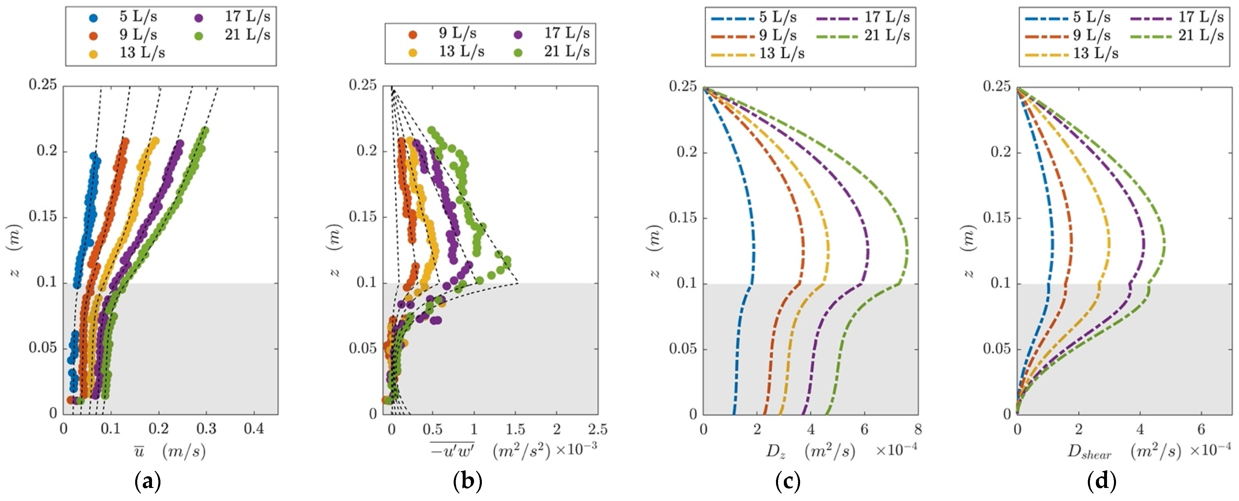
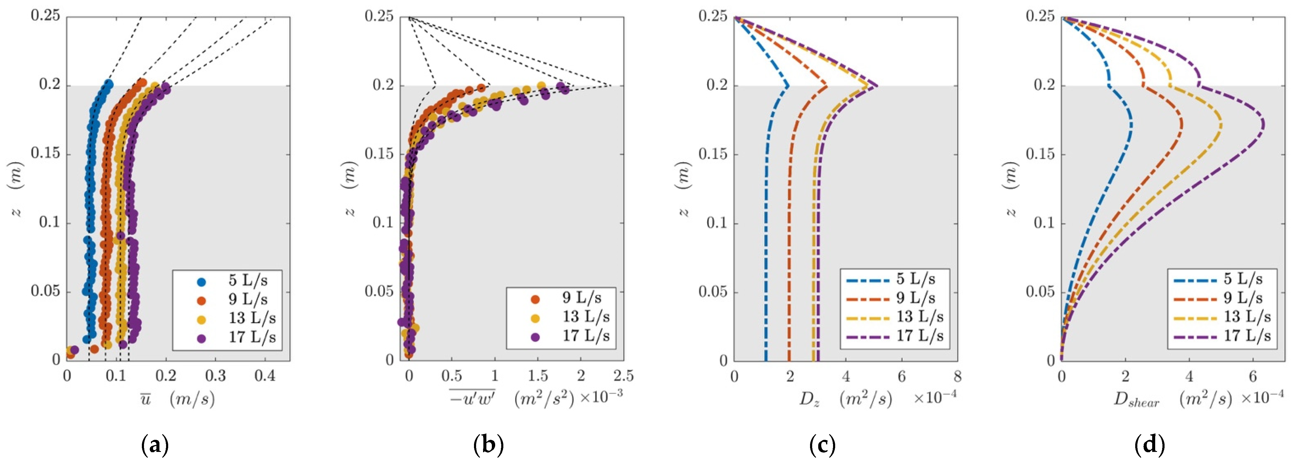
The unavailability of velocity measurements in the upper part of the water column is a limitation of this study due to the nature of the ADV. Therefore, the line drawn for the available data points was extrapolated to obtain an approximate estimation of the velocities in that region. When the flow rates were compared to the velocity measurements, it was suggested that larger velocity values, such as the ones extrapolated, should prevail in the upper part of the water column to sustain the flow rates. Figure 3a and Figure 4a present the measured and fitted velocity profiles for different tested flow rates. When the velocity profiles between the two canopy conditions are compared, the velocity profile from the canopy height at 0.2 m consists of a larger velocity shear towards the top of the canopy.

4.2. Shear Stress Profile

Viscous stress component $({\tau }_v)$ was added to the turbulent stress component $({\tau }_r)$ to obtain the shear stress $\left(\tau \right)$. However, the turbulent stress component dominated the magnitude of the shear stress in the tested flow conditions.

When calculating the viscous shear stress, the kinematic viscosity was chosen based on the water temperature measured with the ADV. The velocity gradient was calculated from the fitted velocity profile obtained from the velocity model explained in Section 4.1.

The turbulent shear stress was obtained from the Reynolds stress. A mixing length approach was used for modelling the turbulent stress profile inside the canopy. The velocity measurements in the “weak spot” were ignored when calculating the Reynolds stress profile and the mixing length.

Several mixing length theories are available in the literature. Equation (12) [48] indicates that the turbulent shear stress is related to the velocity gradient,

$${\tau }_r=-\rho \overline{u^{\prime }{w}^{\prime }}=\rho \left[l^2\right]\left(\left|\frac{\partial u}{\partial z}\right|\frac{\partial u}{\partial z}\right)$$

(12)

where $l$ is the mixing length.

Equation (13) [49] shows that the turbulent shear stress is related to the first and second derivatives of the velocity profile with respect to $z$,

$${\tau }_r=-\rho \overline{u^{\prime }{w}^{\prime }}=\rho {\kappa }^2{\left(\frac{\partial u}{\partial z}\right)}^4/{\left(\frac{{\partial }^{2}u}{\partial z^2}\right)}^2$$

(13)

where $\kappa$ is the von-Karman constant.

Equation (14) [47,50,51] depicts that the Reynolds stress is related to the velocity and velocity gradient,

$${\tau }_r=-\rho \overline{u^{\prime }{w}^{\prime }}=\rho \lambda \left(u\frac{du}{dz}\right)$$

(14)

where $\lambda$ is a characteristic turbulent length scale.

The turbulent stresses measured inside the canopy and the functions of the velocity derivatives were plotted to verify the applicability of Equations (12)–(14). It was observed that the gradient corresponding to mixing length $\lambda$ in Equation (14) remains constant throughout the region inside the canopy, while the gradient corresponding to mixing length $l$ in Equation (12) varies along the canopy. Equation (13) was unable to produce accurate estimations for the tested conditions. It was also observed that the magnitude of $\lambda$ remains consistent for different flow rates when the canopy properties remain unchanged. This observation complements previous findings on the magnitude of $\lambda$ being dependent only on water depth and vegetation height [47,51]. For a constant water depth of 0.25 m and canopy height of 0.1 m, the averaged mixing length $\left(\lambda \right)$ is 5.6 mm, with an NRMSE of 6.7%. For a canopy height of 0.2 m, the average mixing length $\left(\lambda \right)$ is 2.5 mm, with an NRMSE of 3.3%.

Figure 5 presents the calculated $\lambda$ values for each canopy submergence vs. canopy height in each test condition, $h_c=$ 0.1 m and $h_c=$ 0.2 m. There are few empirical estimations of $\lambda$ in the literature. The first empirical relationship (ER1) mentions that the mixing length can be approximated with $0.0144\sqrt{h{h}_c}$ [51]. The second empirical relationship (ER2) states that the mixing length can be approximated with $h_w/20$ [52]. The third empirical relationship (ER3) suggests that the mixing length can be approximated with $0.03\sqrt{h_w{h}_c}$ [47]. The mixing lengths obtained for different canopy heights from these three empirical relationships are also plotted in Figure 5 for a constant water depth of 0.25 m. According to Figure 5, the three empirical equations produce close estimations when the submergence ratio is low ($h_c=0.2$ m). For the canopy height of 0.1 m, $\lambda$ values derived from empirical relationships vary from those calculated from the measurements. Given that this study was conducted only for two canopy heights and one water depth, herein, the attempts are not made to suggest an empirical relationship for $\lambda$.

Once $\lambda$ is established, the turbulent shear stress inside the canopy was evaluated using Equation (8). The turbulent shear stress above the canopy was calculated using existing knowledge; the maximum shear occurs at the top of the vegetation canopy and linearly decays to zero at the air-water interface. Figure 3b and Figure 4b present the measured and fitted profiles of $-\overline{u\text{'}w\text{'}}$ for the tested flow rates. The shear stress is negligible inside a canopy of 0.2 m; however, it drastically peaks at the top to reach a higher value when compared to a canopy of 0.1 m.

4.3. Longitudinal Dispersion Measurements

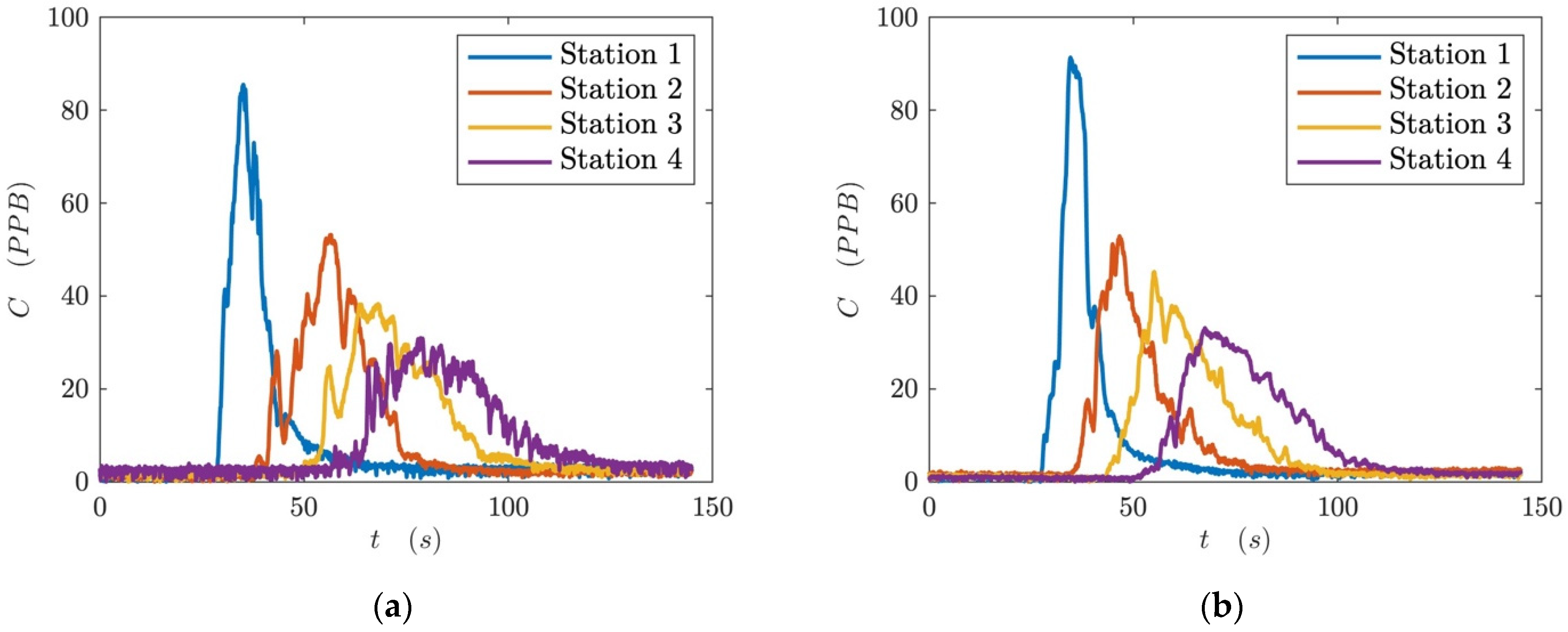
The coefficient of longitudinal dispersion $\left(D\right)$ was experimentally derived based on the temporal variance of the injected tracer cloud measured along the distance through the canopy, using Equation (3). The average velocity of the cloud $\left(u\right)$ was calculated based on the time taken for the centroid of the tracer cloud to move from the first station to the fourth. Figure 6 presents a typical tracer measurement, where Figure 6a denotes the concentration measurements collected using the fluorometers located inside the canopy, and Figure 6b indicates the concentration measurements above the canopy for the canopy height of 0.1 m. The concentration time series measured inside the canopy consists of more scatter compared to the concentration time series measured above the canopy. The peak concentrations measured using the fluorometers inside the canopy are slightly lower than those measured above the canopy, as the bottom fluorometers might miss the solute movement in the upper part of the water column.

Table 1. Experimentally derived characteristic mixing length scale and coefficient of longitudinal dispersion for different flow conditions.

${\mathit{h}}_{\mathit{c}}$(m)	$\mathit{Q} \left(l/s\right)$	$\mathit{\lambda } \left(\mathrm{mm}\right)$	Measured inside the Canopy		Measured above the Canopy		$\mathbf{Calculated} \mathit{D}\left(\mathit{N}\right)$ $\mathbf{from} \mathbf{the} \mathbf{N}-\mathbf{Zone} \mathbf{Model}$ $\left(\times {10}^{-2}{m}^2/s\right)$
			$\mathbf{Average} {\mathit{D}}_{\mathit{b}}$ $\left(\times {10}^{-2}{m}^2/s\right)$	${\mathit{\sigma }}^2$$\mathbf{of} {\mathit{D}}_{\mathit{b}}$ $\left(\times {10}^{-6}{m}^4/s^2\right)$	$\mathbf{Average} {\mathit{D}}_{\mathit{t}}$ $\left(\times {10}^{-2}{m}^2/s\right)$	${\mathit{\sigma }}^2$$\mathbf{of} {\mathit{D}}_{\mathit{t}}$ $\left(\times {10}^{-6}{m}^4/s^2\right)$
0.1	5	-	1.23	3.35	1.75	1.39	1.69
	9	6.2	2.02	5.71	2.84	5.37	2.61
	13	5.2	2.69	7.10	3.79	5.45	4.41
	17	5.4	4.06	22.97	5.55	3.97	6.09
	21	5.5	5.20	24.69	7.10	9.96	7.09
0.2	5	-	0.47	0.77	1.97	1.13	2.56
	9	2.5	0.71	0.72	3.65	27.73	4.37
	13	2.6	0.80	2.87	5.06	5.61	5.80
	17	2.4	1.40	14.89	7.37	64.98	7.34

presents the magnitudes of $\lambda$ and the coefficients of longitudinal dispersion derived inside $\left(D_b\right)$ and above $\left(D_t\right)$ the canopy for different vegetated flow conditions. Five repeat injections were conducted for each test condition, and the average and variance of the longitudinal dispersion coefficients were reported. Here, $D_b$ does not provide a dispersion coefficient for the whole cross-section as the fluorometers inside the canopy miss out on some of the tracer movements above the canopy. Therefore, $D_b$ may only be used for discussing the magnitude of the vertical mixing in each canopy configuration.

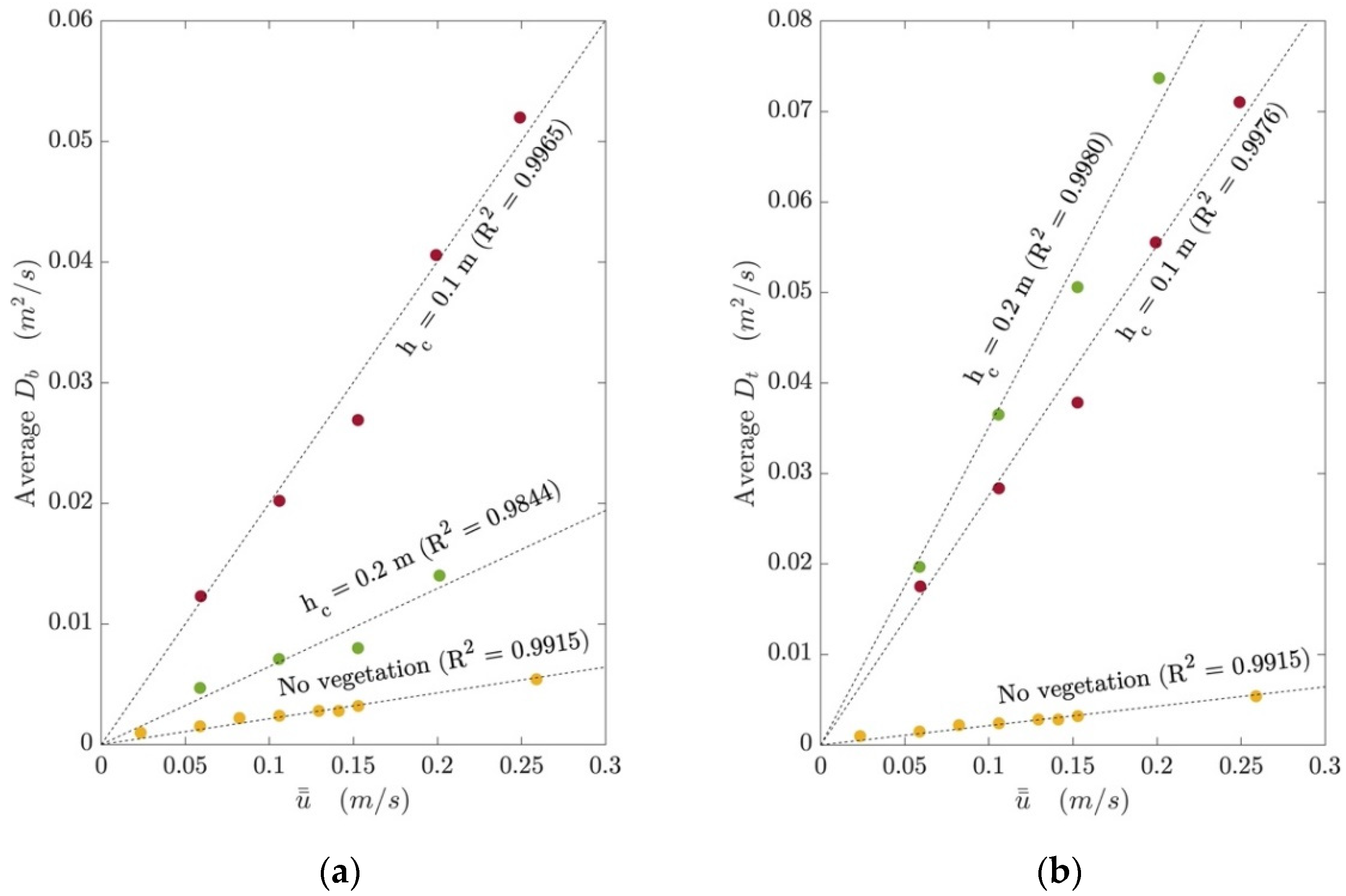
Figure 7 presents the data in Table 1 against the depth-averaged mean velocity $\left(\stackrel{=}{u}\right)$: $D_b$ is plotted in Figure 7a and $D_t$ is plotted in Figure 7b. The coefficient of longitudinal dispersion measured in control tests without vegetation is also plotted to comprehend the effect of vegetation (in the absence of canopies, a single tracer measurement was collected for each cross-section at the mid-water depth). The best-fit lines are drawn through the origin, as the magnitude of molecular diffusion is negligible compared to the magnitudes of turbulent diffusion and shear dispersion. According to Figure 7, the magnitude of $D_b$ is smaller than $D_t$ for both canopy heights. This observation is expected, as the fluorometers inside the canopy observe a reduced velocity and turbulence compared to the upper part of the water column. This observation confirms that vertical mixing is not strong enough to create a uniform solute distribution throughout the cross-section [32]. All longitudinal dispersion measurements in vegetated conditions $(D_b$ and $D_t)$ are significantly greater than those measured in open channel flow. Here, the longitudinal dispersion measurements $\left(D_t\right)$ for the canopy heights of 0.1 m and 0.2 m are ~12 and 15 times the longitudinal dispersion coefficients obtained for open channel flow, respectively. This observation complements the increased shear dispersion in vegetated flows compared to open channel flow. The canopy height of 0.2 m causes the highest value of $D_t$, and the canopy height of 0.1 m produces the highest value of $D_b$, when the two canopies are compared. Even though the canopy height of 0.2 m has increased the longitudinal dispersion in the cross-section, this enhancement does not seem to be uniform over the water depth.

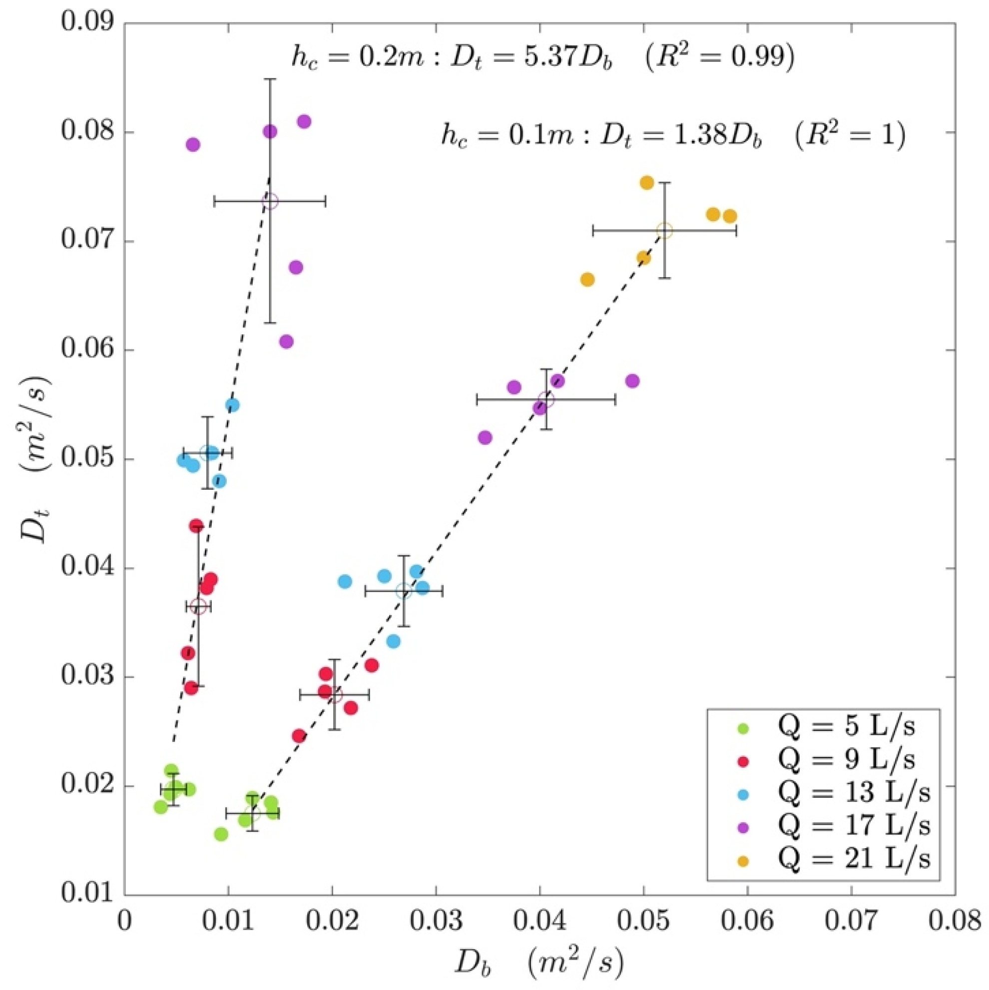
Figure 8 compares $D_b$ and $D_t$ with each other for two tested canopies, and $D_t$ remains consistently proportional to $D_b$ at different flow rates. $D_t/D_b$ depend on the canopy height: 1.4 for $h_c$ = 0.1 m ($h/h_c=$ 2.5), and 5.4 for $h_c$ = 0.2 m ($h/h_c=$ 1.25), despite the constant 0.125 m distance between the top and bottom fluorometers. It is generally observed that the variance of $D_t$ and $D_b$ is high when the measuring point is located near the canopy edge. The complexity of flow dynamics in canopy boundaries may cause this behaviour. The presence of vortices can affect the tracer movement, and the tracer can also become trapped at the surface of canopy elements and eventually be released into the flow, which might not be precisely repeatable. Hence, repeated testing is recommended for dispersion measurements in the boundaries of different flow regimes, as a practical measure even for consistent vegetation canopies.

4.4. Application of the N-Zone Model

4.4.1. Obtaining Horizontal and Vertical Diffusivity Profiles

The diffusivities were calculated using Equation (7) assuming a turbulent Schmidt number equal to unity ($S_{cT}$ = 1). Since isotropy is assumed, the magnitudes of horizontal and vertical diffusivities were similar. The vertical diffusivity profiles obtained for the tested flow conditions are plotted in Figure 3c and Figure 4c. Since the diffusivities are approximate estimations calculated based on velocity measurements, the profiles were plotted using dotted lines. The diffusivity profiles consist of sharp edges in their shape as they inherit the imperfections of the assumptions made when fitting the velocity models. The diffusivities reach a maximum slightly above the canopy ($h_c=$ 0.1 m) or at the top of the canopy ($h_c=$ 0.2 m) and gradually decrease when going into the canopy. Overall, the magnitude of the vertical diffusivity at $h_c=$ 0.1 m is higher than that at $h_c=$ 0.2 m.

4.4.2. Calculating the Coefficient of Longitudinal Dispersion

When the diffusivity and the velocity profile were known, the coefficient of longitudinal dispersion was calculated using Equations (9) and (10). The first term in Equation (9) calculates the longitudinal dispersion occurring due to the velocity shear, i.e., differential advection. The second term calculates the longitudinal dispersion occurring due to turbulent diffusion.

When calculating the diffusivity and applying the N-zone model, the fitted velocity profiles (shown in Figure 3a and Figure 4a) and the fitted shear stress profiles (shown in Figure 3b and Figure 4b) were used for obtaining the velocity gradient, diffusivity, and the velocity in each cell. If scattered raw measurements of the velocity profiles were used in the N-zone model to evaluate longitudinal dispersion, it would be interpreted as higher velocity gradients between zones, resulting in overestimations of shear dispersion. Here, a calculated velocity model and a shear stress profile based on a calibrated mixing length were used to avoid overestimating the shear dispersion. For the test conditions, the shear dispersion was three orders of magnitude larger than the turbulent diffusion in each cell. Therefore, the turbulent diffusion is not presented here, and the contribution from each zone in the water column for shear dispersion is presented in Figure 3d and Figure 4d. The profiles were plotted using dotted lines because they are only approximate estimations. Here, the shear dispersion is maximum in the middle region of the water column, roughly around the upper part of the vegetation canopy, where the velocity gradient is also at its maximum.

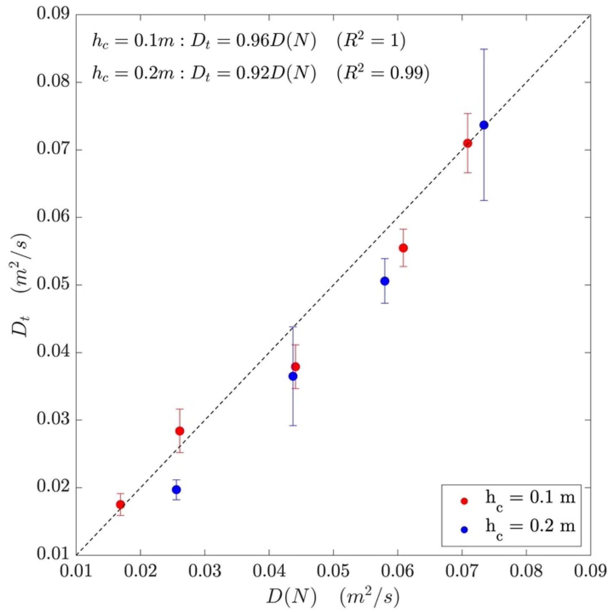
Table 1 summarises the coefficients of longitudinal dispersion estimated using the N-zone model $\left(D\left(N\right)\right)$. $D\left(N\right)$, which is evaluated using the N-zone model, is compared with the coefficient of longitudinal dispersion measured above the canopy $\left(D_t\right)$ in Figure 9. The N-zone model has produced acceptable estimations, with an average overestimation of 6.4%.

5. Discussion

5.1. Vertical Mixing in the Presence of Submerged Canopies

Vertical diffusivity contributes to the first term in Equation (9) which is the shear dispersion. Shear dispersion is significantly larger than turbulent diffusion (second term in Equation (9)) which depends on horizontal diffusivity. According to Figure 3 and Figure 4, the vertical diffusivity is generally higher throughout the cross-section for the canopy height of 0.1 m, compared to the canopy height of 0.2 m. This suggests that better cross-sectional mixing occurs when the canopy height is 0.1 m, and this observation on diffusivity profiles generated based on velocity measurements complements the experimental observations from tracer measurements. According to Figure 8, for a 0.1 m canopy height, the magnitude of longitudinal dispersion obtained from tracer measurements inside the canopy is very close to that measured above. However, the longitudinal dispersion measured from tracer measurements inside the canopy of 0.2 m is one-fifth of that measured above the canopy.

Previous research on submerged vegetation discusses the occurrence of a vertical mixing layer in the upper part of the submerged canopy. The rate of vertical transport in the bottom part of the canopy is dominated by stem-wake turbulence [28], which is an order of magnitude lower than the rate of vertical transport in the upper part of the canopy [23]. The thickness of the vertical exchange zone in the upper part of the canopy $\left({\delta }_e\right)$ can be approximated with $\left(0.23\pm 0.06\right)/\left(C_{D}a\right)$ when $C_{D}ah\ge 0.1$ [30], where $C_D$ is the drag coefficient and $a$ is the leaf area index of the canopy. Taking $C_D\approx 1$, the thickness of the vertical exchange zone is given by 53 mm $\le {\delta }_e\le$ 91 mm for the tested canopy layout in this study. This suggests that the vertical mixing layer reaches beyond the bottom fluorometer when the canopy height is 100 mm as the fluorometer is located 50 mm below the top of the canopy. However, for the canopy height of 200 mm where the fluorometer is located 100 mm below the top of the canopy, the vertical mixing layer does not reach the position of the bottom fluorometer.

5.2. Longitudinal Dispersion in the Presence of Submerged Canopies

Figure 3 and Figure 4 provide a comprehensive description in terms of the hydrodynamic conditions and shear dispersion for the two tested submerged canopies. Overall, the velocities in the canopy are lower, compared to the velocities in the free-flowing region above the canopy, for both canopy conditions. When compared, the peaks in the velocity profile and the shear stress profile of the canopy height of 0.1 m do not reach as high as the canopy height of 0.2 m, even though they comprise noticeable magnitudes throughout the water column. Accordingly, the vertical diffusivities are significantly higher for the canopy height of 0.1 m. Based on the velocity profile, the canopy height of 0.2 m creates the highest differential advection. In addition, the shear stresses are minimal inside the canopy height of 0.2 m before it increases with a steep gradient to reach a huge peak at the top of the canopy. Accordingly, the vertical diffusivities are lower for the canopy height of 0.2 m, resulting in increased shear dispersion.

5.3. Applicability of the N-Zone Model into Submerged Vegetation

The basis for the N-zone model was the slow-zone model, which divides the flow into two zones: a slow zone and a fast zone [53]. The advantage of the N-zone model over the two-zone model is its ability to fit complex shapes of the velocity profiles by increasing the number of zones. In addition, the contribution from each location in the water column for longitudinal mixing can be obtained using the N-zone model, which can be beneficial in managing environmental pollution problems. Only a limited number of studies have been conducted on the N-zone model to determine the longitudinal dispersion in vegetated flows, and one such study was conducted for natural vegetation [35]. The limited number of studies with the N-zone model might be due to the challenges in deriving accurate values for velocities and turbulent shear stresses in vegetated flows. The benefit of the N-zone model is its ability to link the velocity profile with the mixing characteristics, even when the information for other critical parameters of the canopy, such as the drag coefficient or the characteristics of the mixing layer, is unknown.

During this study, we evaluated the applicability of the N-zone model for two canopy submergences representing two conditions. For $h_c=$ 0.1 m $\left(h/h_c=2.5\right)$, the vertical exchange zone reaches a significant distance into the canopy resulting in an enhanced cross-sectional uniformity of the solute. For $h_c=$ 0.2 m $\left(h/h_c=1.25\right)$, the vertical exchange zone has limited development, causing a higher shear dispersion in the cross-section. Even though these two canopy geometries provided insight into the effect of submergence on longitudinal dispersion, test results from a series of different canopy heights for a constant water depth would provide a better understanding of the optimum canopy height which provides the maximum shear dispersion. If the velocity data were available for different canopy heights, the turbulent stress data can be used for obtaining the mixing length for each canopy condition using the Reynolds analogy, and an empirical relationship for $\lambda$ can be obtained, which will increase the applicability of the N-zone model in future even when turbulence data are unavailable.

The coefficient of longitudinal dispersion is a bulk transport coefficient which includes all the physical processes of the cross-section of the flow. When applying the N-zone model, the flow is assumed to be two-dimensional, ignoring the three-dimensional effect of the flow due to the walls. The unavailability of velocity measurements in the upper part of the water column is also a limitation here, as the three-dimensional effect of the flow might be visible in the velocity and turbulent stress profiles near the air–water interface. This study represents a three-dimensional flow in a simplified two-dimensional model to obtain a bulk transport coefficient which is used in the context of a depth-averaged one-dimensional model. Therefore, the results of this study can be extended using future studies consisting of different aspect ratios of the channels with different wall roughness.

The relatively high error in the velocity measurements at the lower flow rates can affect the accuracy of the estimations of $\lambda$. Since the N-zone model relies on the velocity profile and diffusivities, improvements in calculating accurate velocity profiles and mixing lengths will increase the applicability of the N-zone model. For example, if the diffusivity can be presented as a function of the velocity gradient (as shown in [54,55]), it will be possible to use the N-zone model with more reliable diffusivity values, once the mean velocity profile and velocity gradients are established. The tested canopies in this study were rigid, and tests on flexible canopies will also help with understanding the applicability of the N-zone model for flexible canopies, especially when very flexible canopies obstruct the vertical continuity of the water column.

6. Conclusions

The effect of submerged vegetation on longitudinal dispersion measured in two locations in the water column: inside and above the canopy was experimentally evaluated for two canopy submergences. The longitudinal dispersion measurements for the canopy heights of 0.1 m and 0.2 m are approximately 12 and 15 times the longitudinal dispersion coefficients obtained for open channel flow, due to the increased shear dispersion that resulted from the increased differential velocities of the water column in the presence of submerged vegetation. The coefficient of longitudinal dispersion measured above the canopies is 1.4 and 5.4 times that measured inside the canopies for the canopy heights of 0.1 m and 0.2 m, respectively. This behaviour complements the previous findings, which suggest that a higher canopy submergence results in better vertical mixing within the canopy. To calculate the coefficient of longitudinal dispersion, a mixing length was evaluated based on Reynolds stress measurements for each canopy configuration, the diffusivity profiles were calculated based on the shear stress profiles, and the velocity and diffusivity profiles were applied to the N-zone model. The coefficient of longitudinal dispersion calculated using the N-zone model based on velocity measurements provides a good agreement with the coefficient of longitudinal dispersion measured using the tracer measurements along the vegetated channel. The canopy height of 0.2 m resulted in comparatively smaller vertical diffusivities and a better longitudinal shear dispersion, which is explained by the increased velocity gradients and the increased shear stresses observed towards the top of the canopy. The benefit of this methodology for calculating the coefficient of longitudinal dispersion in the presence of submerged canopies is its ability to produce accurate estimations based on the velocity measurements even when the specific characteristics of the canopy such as the density or flexibility are unknown.

References

1. Green, E.P.; Short, F. World Atlas of Seagrasses; University of California Press: Berkeley, CA, USA, 2003; Volume 47. [Google Scholar] [CrossRef]
2. Westlake, D.F. Aquatic macrophytes and the oxygen balance of running water. SIL Proc. 1922–2010 1961, 14, 499–504. [Google Scholar] [CrossRef]
3. Carpenter, S.R.; Lodge, D.M. Effects of submersed macrophytes on ecosystem processes. Aquat. Bot. 1986, 26, 341–370. [Google Scholar] [CrossRef]
4. Moore, K.A. Influence of Seagrasses on Water Quality in Shallow Regions of the Lower Chesapeake Bay. J. Coast. Res. 2004, 10045, 162–178. [Google Scholar] [CrossRef]
5. Kadlec, R.H.; Wallace, S.D. Treatment Wetlands; CRC Press: Boca Raton, FL, USA, 2008. [Google Scholar]
6. Abdelrhman, M. Effect of eelgrass Zostera marina canopies on flow and transport. Mar. Ecol. Prog. Ser. 2003, 248, 67–83. [Google Scholar] [CrossRef]
7. Chambers, P.; Prepas, E. Nutrient dynamics in riverbeds: The impact of sewage effluent and aquatic macrophytes. Water Res. 1994, 28, 453–464. [Google Scholar] [CrossRef]
8. Schulz, M.; Kozerski, H.-P.; Pluntke, T.; Rinke, K. The influence of macrophytes on sedimentation and nutrient retention in the lower River Spree (Germany). Water Res. 2002, 37, 569–578. [Google Scholar] [CrossRef]
9. Butcher, R.W. Studies on the Ecology of Rivers: I. On the Distribution of Macrophytic Vegetation in the Rivers of Britain. J. Ecol. 1933, 21, 58. [Google Scholar] [CrossRef]
10. Harrod, J.J. The Distribution of Invertebrates on Submerged Aquatic Plants in a Chalk Stream. J. Anim. Ecol. 1964, 33, 335. [Google Scholar] [CrossRef]
11. Gambi, M.; Nowell, A.; Jumars, P. Flume observations on flow density dynamics in Zosteramarina (eelgrass) beds. Mar. Ecol. Prog. Ser. 1990, 61, 159–169. [Google Scholar] [CrossRef]
12. Koch, E.W.; Ackerman, J.D.; Verduin, J.; van Keulen, M. Fluid Dynamics in Seagrass Ecology—From Molecules to Ecosystems. In Seagrasses: Biology, Ecologyand Conservation; Springer: Dordrecht, The Netherlands, 2006; pp. 193–225. [Google Scholar] [CrossRef]
13. Gregg, W.W.; Rose, F.L. The effects of aquatic macrophytes on the stream microenvironment. Aquat. Bot. 1982, 14, 309–324. [Google Scholar] [CrossRef]
14. Sand-Jensen, K.; Mebus, J.R. Fine-Scale Patterns of Water Velocity within Macrophyte Patches in Streams. Oikos 1996, 76, 169. [Google Scholar] [CrossRef]
15. López, F.; García, M.H. Mean Flow and Turbulence Structure of Open-Channel Flow through Non-Emergent Vegetation. J. Hydraul. Eng. 2001, 127, 392–402. [Google Scholar] [CrossRef]
16. Winant, C.D.; Browand, F.K. Vortex pairing: The mechanism of turbulent mixing-layer growth at moderate Reynolds number. J. Fluid Mech. 1974, 63, 237–255. [Google Scholar] [CrossRef]
17. Nepf, H.M.; Vivoni, E.R. Flow structure in depth-limited, vegetated flow. J. Geophys. Res. Oceans 2000, 105, 28547–28557. [Google Scholar] [CrossRef]
18. Ghisalberti, M.; Nepf, H.M. Mixing layers and coherent structures in vegetated aquatic flows. J. Geophys. Res. Atmos. 2002, 107, 3-1–3-11. [Google Scholar] [CrossRef]
19. Nepf, H.M. Flow and Transport in Regions with Aquatic Vegetation. Annu. Rev. Fluid Mech. 2012, 44, 123–142. [Google Scholar] [CrossRef]
20. Nepf, H.M. Flow Over and Through Biota. In Treatise on Estuarine and Coastal Science; Elsevier: Amsterdam, The Netherlands, 2011; Volume 2, pp. 267–288. [Google Scholar]
21. von Kármán, T. Mechanical similitude and turbulence—Reprint from Nachrichten von der Gesellschaft der Wissenschaften zu Göttingen, 1930; National Advisory Committee on Aeronautics: Washington, DC, USA, 1931. [Google Scholar]
22. Okamoto, T.-A.; Nezu, I. Spatial evolution of coherent motions in finite-length vegetation patch flow. Environ. Fluid Mech. 2013, 13, 417–434. [Google Scholar] [CrossRef]
23. Ghisalberti, M.; Nepf, H. Mass Transport in Vegetated Shear Flows. Environ. Fluid Mech. 2005, 5, 527–551. [Google Scholar] [CrossRef]
24. Ikeda, S.; Kanazawa, M. Three-Dimensional Organized Vortices above Flexible Water Plants. J. Hydraul. Eng. 1996, 122, 634–640. [Google Scholar] [CrossRef]
25. Fischer, H.B.; List, E.J.; Koh, R.C.Y.; Imberger, J.; Brooks, N.H. Chapter 4: Shear Flow Dispersion. In Mixing in Inland and Coastal Waters; Academic Press Inc. (London) Ltd.: London, UK, 1979; pp. 81–102. [Google Scholar]
26. Elder, J.W. The dispersion of marked fluid in turbulent shear flow. J. Fluid Mech. 1959, 5, 544–560. [Google Scholar] [CrossRef]
27. Fonseca, M.S.; Kenworthy, W. Effects of current on photosynthesis and distribution of seagrasses. Aquat. Bot. 1987, 27, 59–78. [Google Scholar] [CrossRef]
28. Murphy, E.; Ghisalberti, M.; Nepf, H. Model and laboratory study of dispersion in flows with submerged vegetation. Water Resour. Res. 2007, 43, W05438. [Google Scholar] [CrossRef]
29. Ghisalberti, M.; Nepf, H.M. The limited growth of vegetated shear layers. Water Resour. Res. 2004, 40, W07502. [Google Scholar] [CrossRef]
30. Nepf, H.; Ghisalberti, M.; White, B.; Murphy, E. Retention time and dispersion associated with submerged aquatic canopies. Water Resour. Res. 2007, 43, W04422. [Google Scholar] [CrossRef]
31. Fischer, H.B. The Mechanics of Dispersion in Natural Streams. J. Hydraul. Div. 1967, 93, 187–216. [Google Scholar] [CrossRef]
32. Patil, S.; Li, X.; Li, C.; Tam, B.Y.F.; Song, C.Y.; Chen, Y.P.; Zhang, Q. Longitudinal dispersion in wave-current-vegetation flow. Phys. Oceanogr. 2009, 19, 45–61. [Google Scholar] [CrossRef]
33. Fischer, H.B.; List, E.J.; Koh, R.C.Y.; Imberger, J.; Brooks, N.H. Chapter 2: Fickian Diffusion. In Mixing in Inland and Coastal Waters; Academic Press Inc (London) Ltd.: London, UK, 1979. [Google Scholar]
34. Shucksmith, J.D.; Boxall, J.B.; Guymer, I. Effects of emergent and submerged natural vegetation on longitudinal mixing in open channel flow. Water Resour. Res. 2010, 46, W04504. [Google Scholar] [CrossRef]
35. Shucksmith, J.D.; Boxall, J.B.; Guymer, I. Determining longitudinal dispersion coefficients for submerged vegetated flow. Water Resour. Res. 2011, 47, W10516. [Google Scholar] [CrossRef]
36. Noori, R.; Ghiasi, B.; Sheikhian, H.; Adamowski, J.F. Estimation of the Dispersion Coefficient in Natural Rivers Using a Granular Computing Model. J. Hydraul. Eng. 2017, 143, 04017001. [Google Scholar] [CrossRef]
37. Noori, R.; Mirchi, A.; Hooshyaripor, F.; Bhattarai, R.; Haghighi, A.T.; Kløve, B. Reliability of functional forms for calculation of longitudinal dispersion coefficient in rivers. Sci. Total. Environ. 2021, 791, 148394. [Google Scholar] [CrossRef]
38. Lowe, R.J.; Koseff, J.R.; Monismith, S.G. Oscillatory flow through submerged canopies: 1. Velocity structure. J. Geophys. Res. Atmos. 2005, 110, C10016. [Google Scholar] [CrossRef]
39. Augustin, L.N.; Irish, J.L.; Lynett, P. Laboratory and numerical studies of wave damping by emergent and near-emergent wetland vegetation. Coast. Eng. 2009, 56, 332–340. [Google Scholar] [CrossRef]
40. Thuy, N.B.; Tanimoto, K.; Tanaka, N.; Harada, K.; Iimura, K. Effect of open gap in coastal forest on tsunami run-up—Investigations by experiment and numerical simulation. Ocean Eng. 2009, 36, 1258–1269. [Google Scholar] [CrossRef]
41. Liu, P.L.-F.; Chang, C.-W.; Mei, C.C.; Lomonaco, P.; Martin, F.L.; Maza, M. Periodic water waves through an aquatic forest. Coast. Eng. 2015, 96, 100–117. [Google Scholar] [CrossRef]
42. Abdolahpour, M.; Ghisalberti, M.; Lavery, P.; McMahon, K. Vertical mixing in coastal canopies. Limnol. Oceanogr. 2017, 62, 26–42. [Google Scholar] [CrossRef]
43. Abdolahpour, M.; Hambleton, M.; Ghisalberti, M. The wave-driven current in coastal canopies. J. Geophys. Res. Oceans 2017, 122, 3660–3674. [Google Scholar] [CrossRef]
44. Luhar, M.; Coutu, S.; Infantes, E.; Fox, S.; Nepf, H. Wave-induced velocities inside a model seagrass bed. J. Geophys. Res. Atmos. 2010, 115, C12005. [Google Scholar] [CrossRef]
45. Thomas, R.E.; Schindfessel, L.; McLelland, S.J.; Creëlle, S.; De Mulder, T. Bias in mean velocities and noise in variances and covariances measured using a multistatic acoustic profiler: The Nortek Vectrino Profiler. Meas. Sci. Technol. 2017, 28, 075302. [Google Scholar] [CrossRef]
46. Chikwendu, S.C. Calculation of longitudinal shear dispersivity using an N-zone model as N → ∞. J. Fluid Mech. 1986, 167, 19–30. [Google Scholar] [CrossRef]
47. Tang, X. A mixing-length-scale-based analytical model for predicting velocity profiles of open-channel flows with submerged rigid vegetation. Water Environ. J. 2019, 33, 610–619. [Google Scholar] [CrossRef]
48. Prandtl, L. 7. Bericht über Untersuchungen zur ausgebildeten Turbulenz. ZAMM—Journal of Applied Mathematics and Mechanics/Zeitschrift für Angewandte Mathematik und Mechanik 1925, 5, 136–139. [Google Scholar] [CrossRef]
49. Schlichting, H.; Gersten, K. Boundary-Layer Theory; Springer: Berlin/Heidelberg, Germany, 2016. [Google Scholar] [CrossRef]
50. Klopstra, D.; Barneveld, H.J.; van Noortwijk, J.M.; van Velzen, E.H. Analytical model for hydraulic roughness of submerged vegetation. In Proceedings of the Theme A, Managing Water: Coping with Scarcity and Abundance: The 27th Congress of the International Association for Hydraulic Research, San Francisco, CA, USA, 10–15 August 1997; pp. 775–780. [Google Scholar]
51. Meijer, D.G.; Van Velzen, E.H. Prototype-scale flume experiments on hydraulic roughness of submerged vegetation. In Proceedings of the 28th IHAR World Congress, Graz, Austria, 22–27 August 1999. [Google Scholar]
52. Baptist, M.J.; Babovic, V.; Uthurburu, J.R.; Keijzer, M.; Uittenbogaard, R.; Mynett, A.; Verwey, A. On inducing equations for vegetation resistance. J. Hydraul. Res. 2007, 45, 435–450. [Google Scholar] [CrossRef]
53. Chikwendu, S.C.; Ojiakor, G.U. Slow-zone model for longitudinal dispersion in two-dimensional shear flows. J. Fluid Mech. 1985, 152, 15–38. [Google Scholar] [CrossRef]
54. Boghi, A.; Di Venuta, I.; Gori, F. Passive scalar diffusion in the near field region of turbulent rectangular submerged free jets. Int. J. Heat Mass Transf. 2017, 112, 1017–1031. [Google Scholar] [CrossRef]
55. Di Venuta, I.; Boghi, A.; Angelino, M.; Gori, F. Passive scalar diffusion in three-dimensional turbulent rectangular free jets with numerical evaluation of turbulent Prandtl/Schmidt number. Int. Commun. Heat Mass Transf. 2018, 95, 106–115. [Google Scholar] [CrossRef]
Figure 1. Flow hydrodynamics around submerged rigid aquatic canopies: (a) basic nomenclature of a vegetated open channel flow and the expected shape of the velocity profile; and (b) the shear stress profile and associated mixing processes in a vegetated channel (based on previous work, references provided in the body).
Water 15 03021 g001
Figure 2. Experimental setup (not to scale): the side view of the testing flume, the placement of fluorometers for the two tested vegetation configurations, and the staggered grid layout of vegetation in the plan. In all the diagrams, the flow is from left to right.
Water 15 03021 g002
Figure 3. Hydrodynamics of the water column in the presence of the canopy of 0.1 m height: (a) measured and fitted velocity profiles for the tested flow conditions; (b) measured and fitted profile of u ' w ' ¯ ; (c) estimated diffusivity profiles for the tested flow conditions; and (d) estimated contribution from each zone in the water column on shear dispersion.
Water 15 03021 g003
Figure 4. Hydrodynamics of the water column in the presence of the canopy of 0.2 m height: (a) measured and fitted velocity profiles for the tested flow conditions; (b) measured and fitted profile of u ' w ' ¯ ; (c) estimated diffusivity profiles for the tested flow conditions; and (d) estimated contribution from each zone in the water column on shear dispersion.
Water 15 03021 g004
Figure 5. Variation of λ with vegetation canopy height for a constant water depth of 0.25 m.
Water 15 03021 g005
Figure 6. A typical tracer concentration measurement along the channel (the data corresponds to the flow rate of 17 L/s when the canopy height is 0.1 m): (a) from the fluorometers inside the canopy; and (b) from the fluorometers above the canopy.
Water 15 03021 g006
Figure 7. Measured averaged coefficient of longitudinal dispersion for different flow conditions (with and without a canopy) plotted against the depth averaged mean velocity: (a) measured inside the canopy; and (b) measured above the canopy.
Water 15 03021 g007
Figure 8. Comparison of D evaluated from the measurements above the canopy with D evaluated from the measurements inside the canopy.
Water 15 03021 g008
Figure 9. Comparison of D evaluated from the measurements above the canopy with D (N) evaluated from the N-zone model.
Water 15 03021 g009