SPH Simulation of Sediment Movement from Dam Breaks

Abstract

This study aims to develop a robust sediment transport model focusing on the vertical two-dimensional water–sediment two-phase flow in which sediments are constantly interacting, hitting each other, gradually becoming smoother and smaller, and accumulating when velocities decrease. The grid-based models currently available can be cumbersome when dealing with phenomena that require replication of this water–sediment interface. Therefore, a two-dimensional water–sediment two-phase flow model based on Smoothed Particle Hydrodynamics (SPH) is established in the macroscopic scale to simulate a large amount of sediment accumulation and propagation typical of a landslide caused by a dam break. In this study, water and sediments are treated as two kinds of fluids with different densities and viscosities to accurately simulate the flow structure, the sediment transport, and the water–sediment interaction process. The interaction model developed treats the interface of the two phases within a unified framework. The model developed was then tested against three applications, and the results obtained confirmed its accuracy in correctly replicating the movement of the sediment phase. The preliminary results obtained can be helpful in providing further insights into the mixing of water and sediments and their propagation following a dam break and the consequent wave profile generated.

1. Introduction

Sediment transport in mountainous rivers can affect the formation and shaping of downstream streams and can alter water intake, channel regulation, and flood disaster prevention. The movement characteristics of the sediment transport are discontinuous and complex; thus, its numerical simulation is extremely challenging. Additionally, to make this situation even more difficult, nowadays, many more hydropower projects have been constructed, affecting the natural supply of sediments in natural creeks and rivers [1].

Erosion, entrainment, transportation, deposition, and compaction of sediment carried into reservoirs are all processes typical of unregulated, mature rivers with stable catchments and are relatively balanced. However, the construction of a dam usually decreases the correspondent flow velocities, initiating or accelerating sedimentation and, therefore, resulting in progressively finer materials being deposited and causing the siltation of reservoirs, a problem that affects many hydropower projects across the world.

The operation of these projects also introduces complex changes in the flow movement, and the discontinuity of the sediments is also strengthened, complicating even more its accurate simulation. Water intake and channel regulation can vary based on the variation of non-uniform sediment transport linked with complex flow conditions plus, in worst-case scenarios such as a dam break, the large flow released may contain a variety of sediments that mix with water and generate landslides that can cause severe damage to cities and inhabitants living downstream the hydropower station [2,3]. Municipalities are shaping and implementing several plans to prevent and diminish flood disasters in mountainous rivers, but they require a better understanding of the prominent characteristics of mountainous floods, which are obviously different from traditional floods due to the dissimilar interaction between flow and sediments. In mountainous areas, floods can lead to a sharp rise in water levels in rivers which, linked with steep slopes, can transport high amounts of sediments of various sizes at very intense velocities [4]. A sediment motion layer with a high-speed shear collision is formed near the riverbed, leading to a high-intensity sediment transport rate and the rapid evolution of the riverbed. The described process is very complex and still requires a more accurate and effective numerical simulation to better predict bed–load mixing and transport [5].

Overall, sediment transport is the process of erosion, transport, and accumulation of sediment under the action of water flow and is a common natural phenomenon in rivers [6]. The study of sediment transport is an important topic when investigating both geomorphology and hydraulic dynamics. Understanding the characteristics of the movement of the sediments under different hydrodynamic conditions involves solving urgent scientific questions in unfavorable situations such as irrigation canal siltation, reservoir siltation, harbor and bay estuary siltation, and flash floods causing disasters. For example, on the 8th of August 2017, reported flash floods in Liangshan, Sichuan Province, China, caused by heavy rainfall (Figure 1), generated the transport of copious amounts of sediments, changing the morphology of the existing riverbed [7].

Dam break incidents happen regularly across the world. For example, 32 million cubic meters of mine waste were spilled following the collapse of the Fundão tailings dam in Brazil, causing a severe socioeconomic and environmental impact on the Doce River. Due to this disaster, approximately 90% of the spilled volume settled on floodplains over 118 km downstream of Fundão Dam. A hyper-concentrated flow (≈400,000 mg/L) reached the Doce River, where the flood wave and sediment wave traveled at different celerities over 570 km to the Atlantic Ocean [8]. Another huge disaster was produced by the wave generated by the 270 million cubic meters from Mount Toc, which overtopped the Vajont Dam on the 9th of October 1963, and caused a landslide to travel toward the Piave Valley and the death of 1900 people. The villages downstream of the dam were completely devastated and turned into a flat plain of mud [9].

The main tools used in studies investigating sediment transport include theoretical analysis, prototype observations, physical model tests, and numerical simulations. Of these research methods, the theoretical analysis, is generally applied to simple constant and uniform flow situations. Prototype observations can provide real-time data but are costly in terms of human and financial resources and, in many cases, are difficult to implement due to physical constraints. Physical models are often constrained by site conditions. As a result, more research has been conducted using numerical simulations to predict sediment transport in rivers, and relevant mathematical models have become indispensable tools for studying the process of water and sand movement and predicting the characteristics of sediment transport [8,9,10,11,12,13,14].

Most of the numerical methods to simulate water and sand movement are based on the Eulerian grid method. The main numerical methods for solving the control equations by the Eulerian method generally include the Finite Element Method (FEM) [15], Finite Volume Method (FVM), and Finite Difference Method (FDM) [16]. Although the mesh method has the advantages of fast computational efficiency and better simulation of turbulence, the mesh method is more cumbersome in dealing with large deformations at the interface between the free surface and the water–sand intersection. The commonly used methods for tracing two intersecting interfaces in the mesh method are the VOF method [17] and the Level Set Method [18]. Among them, the VOF method is complicated to reconstruct the interface, and the Level Set method shows rounding at sharp corners and requires the construction of a higher-order format, which can cause longer computation time and less accurate volume conservation compared to the VOF method. In addition, the grid method is more difficult to accurately model sediment particles, and most models adopt diffusion equations to approximate the distribution of the sediments, an approach that can introduce large errors.

In recent years, a numerical method that does not require a grid, the particle method, has been rapidly developed. The particle method uses a series of discrete points to discretize the entire computational domain and does not suffer from some of the drawbacks and computational difficulties associated with the grid method due to the presence and deformation of the grid, thus giving the particle method an advantage over the grid method in dealing with problems in the field of fluid mechanics such as moving matter intersections and deformable boundaries [19]. The most common particle method schemes are the Weakly Compressible Smoothed Particle Hydrodynamics (WCSPH), Incompressible Smoothed Particle Hydrodynamics (ISPH) and Moving Particle Semi-implicit (MPS) methods. They are widely used in the study of free surface flows [20], non-Newtonian fluids [21,22], and water–sand interactions such as scouring problems [23,24]. The SPH method is one of the simplest and most efficient meshless methods commonly used today. The sediment transport problem in open channels involves the interaction of sediment and water, as well as the treatment of free surfaces, and is a multi-phase problem. At the macroscopic level, the process involves sediment transport and deposition. At the microscopic level, the process involves momentum transfer at the interface, sediment–fluid–turbulence interactions, and stratification processes near the bed surface. Due to the discrete nature of the particles, the SPH method has advantages in modeling large deformation flows and granular materials (e.g., sediment); hence, the SPH method is being used more frequently to simulate water–sand interactions.

There are dissimilar main approaches for SPH modeling of water–sand interactions. For the first one, the two-fluids model uses two particles to represent two fluids and considers a control cell at the microscopic level to be filled by both fluids simultaneously, i.e., both particles can fill the whole computational region or occupy a single point position in space at the same time. The physical situation of this model is consistent with that of the continuous medium model and draws on the results of it which was used by Bui et al. [25], to simulate the development of a jet washout crater caused by a vertical jet under two different initial conditions in saturated and dry soils, taking into account the pore water pressure and infiltration pressure between water and sand.

For the second approach, the two-fluids model uses two sets of particles with different physical properties to represent two mutually immiscible fluids. The two particles move according to their respective controlling equations, and at the two-phase intersection, an interaction model is introduced to simulate the two-phase pressure and shear stress, which is the most widely used two-phase flow model. Pahar and Dhar [26] applied this theory, considering the water pressure, viscous force, and fluid drag force on sediment particles at the two-phase intersection, neglecting the effect of pore pressure and the variation of sediment concentration, and simulated the scouring of the dam break process based on the ISPH method.

Ulrich et al. [27] applied SPH parallel computation to simulate the fall of an offshore wind turbine foundation installation and the scouring of the seabed caused by the operation of a ship’s propeller at realistic scales. Fourtakas and Rogers [24] simulated the three-dimensional (3D) dam break scour problem with four million particles based on parallel computing. Ran et al. [23] simulated the dam break process based on the ISPH method. The model did not involve the input flow, so the particles in the water–sand two-phase flow model were specifically classified into five types: inner water particles, scoured particles, impenetrable wall particles, interface contact particles, and dummy particles. Considering the lateral flow velocity along the bed surface and the vertical impact of the water flow to the bed surface, the moveable bed scouring process caused by the dam break is simulated by judging the critical pick-up flow velocity.

Wang et al. [28] considered the inlet and outlet flow processes and defined six types of particles in the ISPH framework: clear water particles, turbid water particles, interface wall particles, dummy particles, inlet particles, and outlet particles. The initial sediment initiation was judged by comparing the water flow shear stress acting on the wall particle with the critical initiation shear stress, and the formation of a scour pit behind the seawall was simulated.

Manenti et al. [29] simulated the sediment scour process caused by an outflow from the bottom of a reservoir, and bed shear was obtained by calculating the difference between the velocity of the bed particle and the one of the moving water particle close to the bed particle, comparing the Mohr–Coulomb and Shields erosion criterions, and concluded that the Shields erosion criterion could better express the dynamic properties of the sediment.

Unlike the above two water–sand models that use two sets of particles to represent each of the two fluids, for the third approach, the sand-containing water flow is discrete into a set of SPH particles, i.e., the two fluids are mixed as a whole phase, and only one SPH particle is used to describe the two phases of water and sand, considering the variation of the volume fraction of each phase. Each particle carries physical information such as velocity, density, concentration, and pressure of the mixed phase.

Shi [30] used the SPH mixed-phase model to simulate the sediment dumping problem under static water in dredging projects. The model rewrites the two-phase control equation as a control equation for the particle equation of motion and the physical quantities, such as the concentration of the sediment it carries, and investigates the variation of the width, settling velocity, and concentration distribution of the sediment cloud with the sediment particle size and the initial volume of the cloud. To address the problem that this model is not accurate enough in simulating the stresses among sediment particles and drag forces at the intersection interface under high concentration conditions, Shi et al. [31] further incorporated a rheological constitutive model based on dense particle flow to describe the stresses among particles and used the Gidaspow formula to calculate the drag forces at the intersection interface at different concentrations to simulate the collapse of a submerged particle in static water and dam break on a dynamic bed.

The water–sand two-phase flow model developed in this paper is based on the third idea, using the SPH method to discretize the turbulent mean control equation and simultaneously solve the turbulent closure model and the stresses among sediment particles [32] to simulate the water–sand coupling during a dam break. This approach has been widely and successfully used in the grid-based modeling of two-phase flows, particularly within the OpenFOAM framework [32].

The advantage of the mesh method is that it is computationally efficient and can simulate problems on large time scales, while the particle method can facilitate the simulation of large local deformation problems as it does not require the division and reconstruction of the mesh. Both methods have their own advantages and disadvantages when modeling fluid problems, and therefore, this approach was adopted for this study in order to improve the modeling of water–sediment mixing and transport associated with landslides caused by dam break scenarios.

2. Fundamental SPH Formulations

The SPH formulation is a purely meshless Lagrangian method, which is not constrained by the mesh during computation and, therefore, does not cause computational errors due to distortion of the mesh when calculating large deformation problems. The basic idea is to divide the continuous fluid into a series of interacting particles, describe the continuous flow field through discrete particles, and convert the information between the discrete particles and the continuous flow field through the kernel function.

The core theory of the SPH formulations includes kernel approximation, particle approximation, the discretized form of the control equations (discretization of the control equations by the particle approximation), and some numerical processing techniques. The SPH formulations were firstly proposed for solving three-dimensional open-space astrophysics problems [33,34]. Its application in the field of hydraulics was to solve the Navier–Stokes equations via the SPH formulations, which was firstly applied to the simulation of free surface flow by Monaghan [35]. Compared with the traditional mesh method, the SPH formulations have some advantages that the mesh method does not have, despite its relatively brief history of development.

In the particle method, the entire computational domain is discretized into particles, which carry physical information such as velocity, density, mass, and pressure. The next step is to introduce the particle approximation method involved in the construction of the SPH discrete equations, i.e., the kernel approximation equations are further approximated by dispersed particles, the core idea of which is to solve the integral expression by superimposing the summation discretization form of all particles in the support domain. The process of particle superposition is also known as the particle approximation method. The volume of each small part of the problem domain is concentrated on the corresponding discrete particles so that each particle i corresponds to a fixed volume $\Delta V_i$ but does not have a fixed shape. The volume $\Delta V_i$ can be expressed as the ratio of the mass to the density of the corresponding particle. These particles can be either fixed (wall particles) or moving (fluid particles).

3. Standard SPH Fluid Model

The controlling equations for modeling free-surface flow in the two-dimensional (2D) case include the mass conservation equation and the momentum conservation equation, which have the following Lagrangian forms:

$$\frac{1}{\rho }\frac{D\rho }{Dt}+\nabla \cdot \overrightarrow{u}=0$$

(1)

$$\frac{D\overrightarrow{u}}{Dt}=-\frac{1}{\rho }\overrightarrow{\nabla }P+\overrightarrow{g}+\overrightarrow{\Theta }$$

(2)

where ρ is the density; t is time; $\overrightarrow{u}=\left(u,v\right)$is the particle velocity in the 2D case; P is the pressure; and $\overrightarrow{\Theta }$ is the diffusion term.

In this paper, fluids in the form of SPH are considered weakly compressible fluids, and the equation of state is used to relate the density change to the pressure, which allows the pressure to be obtained explicitly without solving the matrix and is faster than solving the Poisson equation for pressure. The use of the equation of state is limited by two conditions. Firstly, compressibility must be commensurate with the reduction in sound speed to rationalize the time step of the model. Secondly, the speed of sound should be ten times the maximum fluid velocity, and as can be seen from Equation (3), minor changes in density can cause large fluctuations in pressure values, so the density needs to be kept within 1% of the variation. The relationship between pressure and density, as proposed by Monaghan and Kos [36], is as follows:

$$\mathrm{P}=\mathrm{B}\left[{\left(\frac{\rho }{{\rho }_0}\right)}^{\kappa }-1\right]$$

(3)

where k = 7; ${\rho }_o=$1000 kg/m³ is the initial density; the constant $B=\frac{c^2{\rho }_o}{\gamma }$, of which $c=10\times V$max; $V$max is the maximum flow velocity.

The density ${\rho }_i$ of fluid particle i is calculated as follows:

$${\rho }_i={\displaystyle \sum _j{m}_{j}W(}\left|r_i-r_j\right|,h)$$

(4)

where h is the smooth length, and W is the interpolation kernel function. To balance computational accuracy and efficiency in two dimensions, the kernel function uses a segmented cubic spline function [37].

The particle pressure gradient is calculated as follows:

$${(\frac{1}{\rho }\nabla P)}_i={\displaystyle \sum _j{m}_j(\frac{P_i}{{\rho }_i^2}+\frac{P_j}{{\rho }_j^2})}{\nabla }_i{W}_{ij}$$

(5)

where the summation is the sum of all water particles except particle i; ${\nabla }_i{W}_{ij}$ is the gradient of the kernel function with relation to the position of particle i.

The diffusion term is the laminar viscosity term, so that:

$${\overrightarrow{\Theta }}_i={\displaystyle \sum }_j{m}_j\left(\frac{4{\upsilon }_0{\overrightarrow{r}}_{ij}{\nabla }_i{W}_{ij}}{\left({\rho }_i+{\rho }_j\right){\left|{\overrightarrow{r}}_{ij}\right|}^2}\right){\overrightarrow{u}}_{ij}$$

(6)

where ${\upsilon }_o={10}^{-6}{\mathrm{m}}^2/\mathrm{s}$ is the coefficient of laminar motion viscosity; $\overrightarrow{r_{ij}}=\overrightarrow{r_i}-\overrightarrow{r_j}$, $\overrightarrow{r}$ is the position vector.

4. Two-Phase SPH Water–Sediment Model

This section presents the governing equations of the two-phase SPH model and their particle discretization.

4.1. Lagrangian Form of Governing Equations

The following is a set of equations in the Lagrangian form representing water and sand mass and momentum conservation. These are derived from the local instantaneous mass and momentum equations for either phase of water and sand in the two-fluid model. The result is a set of equations in the Lagrangian for representing water and sand mass and momentum conservation, as follows.

(i)

Equation for conservation of mass of water flow:

$$\frac{D({\alpha }^f{\rho }^f)}{Dt}=-{\alpha }^f{\rho }^f\nabla \cdot {\overrightarrow{u}}^f$$

(7)

(ii)

Conservation of momentum equation for water flow:

$$\frac{D{\overrightarrow{u}}^f}{Dt}=-\frac{1}{{\rho }^f}\nabla P^f+\frac{1}{{\alpha }^f{\rho }^f}\nabla \cdot {\overrightarrow{\tau }}^f+\overrightarrow{g}-\frac{{\alpha }^s}{{\rho }^f}K({\overrightarrow{u}}^f-{\overrightarrow{u}}^s)+\frac{1}{{\rho }^f}{S}_{US}K{\upsilon }_t^f\nabla {\alpha }^s$$

(8)

(iii)

Sediment mass conservation equation:

$$\frac{D{\alpha }^s}{Dt}=({\overrightarrow{u}}^f-{\overrightarrow{u}}^s)\cdot \nabla {\alpha }^s-{\alpha }^s\nabla \cdot {\overrightarrow{u}}^s$$

(9)

(iv)

Conservation of sediment momentum equation:

$$\begin{array}{l}\frac{D{\overrightarrow{u}}^s}{Dt}=-\frac{1}{{\rho }^s}\nabla P^f-\frac{1}{{\alpha }^s{\rho }^s}\nabla {\tilde{P}}^s+\frac{1}{{\alpha }^s{\rho }^s}\nabla \cdot {\overrightarrow{\tau }}^s+\overrightarrow{g}+\frac{{\alpha }^f}{{\rho }^s}K({\overrightarrow{u}}^f-{\overrightarrow{u}}^s)\\ -\frac{{\alpha }^f}{{\alpha }^s{\rho }^s}{S}_{US}K{\upsilon }_t^f\nabla {\alpha }^s+({\overrightarrow{u}}^f-{\overrightarrow{u}}^s)\cdot \nabla {\overrightarrow{u}}^s\end{array}$$

(10)

where $t$ is the time; ${\alpha }^f$ is the volume fraction of the water phase; ${\alpha }^s$ is the volume fraction of the sand phase; ${\alpha }^f+{\alpha }^s=1$: ${\rho }^f$ is the density of water, taking into account the weak compressibility of the fluid; ${\rho }^f$ is a variable value; ${\rho }^s$ is the density of sand as a constant value; $\overrightarrow{u^f}$ is the velocity of the water phase; $\overrightarrow{u^s}$ is the velocity of the sand phase; $P^f$is the pressure of the water; $\overrightarrow{{\tau }^f}$ is the shear stress of the flow, including viscous and turbulent terms; $\widetilde{P^s}$ is the positive stress of the sediment phase; $\overrightarrow{{\tau }^s}$ is the shear stress of the sediment phase; ${\upsilon }_t^f$ is the turbulent viscosity coefficient; K is the drag force coefficient; $\overrightarrow{g}$ is the acceleration of gravity; $S_{US}$ is the reciprocal of Schmidt’s number, that is $S_{US}=1/{\sigma }_c$. The Schmidt’s number in this paper takes a value between 0.2 and 1.0, so $S_{US}$ takes a value in the range of 1 to 5. A value of 1 indicates a low drag force, and a value of 5 indicates a high drag force.

The system of the equations has been derived based on the mixture theory. In this system, both the fluid and solid phases are modeled macroscopically, i.e., as continuous media, and the effect of turbulence is modeled through the use of Large Eddy Simulation (LES). Since the discretization of the computational domain is not very fine due to computational cost reasons, the treatment of the turbulence model may not be as exact as when the domain is modeled microscopically. However, in the present applications, the flows are not highly sheared thus, the model performance is good, as shown in Section 5. For more detail on the issue, see Kazemi et al. [38].

4.2. SPH Discretizations in Two-Phase Equations

In the SPH method, the sand-containing flow is discrete into a series of free-moving and interacting particles. The motion of the particles is calculated as the velocity of the water phase, and a particle contains both the physical properties of the water phase and the physical properties of the volume fraction of the sand phase and the velocity of the sand phase. The conventional particle volume is calculated by the following equation:

$$\Delta V=\frac{m}{\rho }$$

(11)

where $\Delta V$ is the volume of the particle; m is the mass of the particle; $\rho$ is the density of the particle. Assuming that a particle contains only the volume fraction of water, then $\Delta V=\frac{m^f}{{\alpha }^f{\rho }^f}=\frac{m^f}{{\rho }^f}$. Assuming that a particle contains only the volume fraction of sand, then $\Delta V=\frac{m^s}{{\alpha }^s{\rho }^s}=\frac{m^s}{{\rho }^s}$. And if a particle contains both water and sand phase, then $\Delta V=\frac{m^s+m^f}{{\alpha }^s{\rho }^s+{\alpha }^f{\rho }^f}$.

Therefore, the following equation can be obtained:

$$\Delta V=\frac{{\alpha }^s{m}_0{}^s+{\alpha }^f{m}_0{}^f}{{\alpha }^s{\rho }^s+{\alpha }^f{\rho }^f}$$

(12)

where $m_0{}^s$ is the single sediment mass, i.e., the mass of a particle when it contains only the sediment phase, and $m_0{}^s={\rho }_0{}^s\Delta V_0$. $m_0{}^f$ is the mass of a single fluid, i.e., the mass of a particle when it contains only the water phase $m_0{}^f={\rho }_0{}^f\Delta V_0$.

Assuming that the sand-containing water flow is a weakly compressible fluid, the sediment is incompressible and therefore ${\rho }_{}{}^s={\rho }_0{}^s$. The fluid phase is weakly compressible and therefore ${\rho }_{}{}^f$ is variable. Apply the equation of state explicitly calculating the pressure of water:

$$P^f=c_0{}^2({\rho }^f-{\rho }_0^f)$$

(13)

where $c_0$ is the speed of sound. As the water flow is assumed to be compressible, the equation of state can be applied to calculate the pressure, but the compressibility should be limited to 1%, so the value of $c_0$ is taken as follows:

$$c_0=10\sqrt{9.81H_0}$$

(14)

where $H_0$ is the initial water depth.

An important element in the SPH time integration is the selection of a suitable time step. In this paper, the time step is calculated according to the Courant–Friedrichs–Lewy (CFL) condition. The basic requirement of the CFL condition is that the minimum value of the particle space is proportional to the time step, and in the SPH approximation calculation, the size of the minimum smooth length is proportional to the time step. In this paper, the CFL is taken as 0.15, which takes into account the computational efficiency and avoids the scattering of results. The value of $\Delta t$ is taken as shown in the following equation:

$$\Delta t\le 0.15\frac{h_{\Upsilon }}{c_0}$$

(15)

where $h_{\Upsilon }$ is taken as 1.2 times the initial particle spacing.

The SPH discretization method is used to discretize the differential terms in the equation into the form of particle summations. In the following, the discretized forms of the equations are presented, where a represents the central particle and b represents the particles in the support domain of the central particle.

(i)

Conservation of water mass:

$$\frac{{\left.{\alpha }_a^f\right|}^{(t+\Delta t)}{\left.{\rho }_a^f\right|}^{(t+\Delta t)}-{\left.{\alpha }_a^f\right|}^{(t)}{\left.{\rho }_a^f\right|}^{(t)}}{\Delta t}={\alpha }_a^f{\rho }_a^f{\displaystyle \sum _b\Delta V_b({\overrightarrow{u}}_a^f-{\overrightarrow{u}}_b^f)}\cdot {\nabla }_a{W}_{ab}$$

(16)

among which $\Delta V_b=\frac{{\alpha }_b{}^s{m}_0{}^s+{\alpha }_b{}^f{m}_0{}^f}{{\alpha }_b{}^s{\rho }_b{}^s+{\alpha }_b{}^f{\rho }_b{}^f}$ and ${\nabla }_a{W}_{ab}=\nabla W(\left|r_a-r_b\right|,h)$.

(ii)

Conservation of water momentum:

$$\begin{array}{l}\frac{{\left.{\overrightarrow{u}}_a^f\right|}^{(t+\Delta t)}-{\left.{\overrightarrow{u}}_a^f\right|}^{(t)}}{\Delta t}=-\frac{1}{{\rho }_a{}^f}{\displaystyle \sum _b\Delta V_b(P_a^f+P_b^f)}{\nabla }_a{W}_{ab}+\frac{1}{{\alpha }_a{}^f{\rho }_a{}^f}{\displaystyle \sum _b\Delta V_b({\overrightarrow{\tau }}_a^f+{\overrightarrow{\tau }}_b^f)}\cdot {\nabla }_a{W}_{ab}\\ +\overrightarrow{g}-\frac{{\alpha }_a{}^s}{{\rho }_a{}^f}{K}_a({\overrightarrow{u}}_a^f-{\overrightarrow{u}}_a^s)-\frac{1}{{\rho }_a{}^f}{S}_{US}{K}_a{\left.{\upsilon }_t^f\right|}_a{\displaystyle \sum _b\Delta V_b({\alpha }_a{}^s-{\alpha }_b{}^s)}{\nabla }_a{W}_{ab}\end{array}$$

(17)

(iii)

Sediment mass conservation:

$$\begin{array}{l}\frac{{\left.{\alpha }_a{}^s\right|}^{(t+\Delta t)}-{\left.{\alpha }_a{}^s\right|}^{(t)}}{\Delta t}=\\ {\alpha }_a^s{\displaystyle \sum _b\Delta V_b({\overrightarrow{u}}_a^s{{}_{}}^{}-{\overrightarrow{u}}_b^s)}\cdot {\nabla }_a{W}_{ab}-{\displaystyle \sum _b\Delta V_b({\alpha }_a^s-{\alpha }_b^s)({\overrightarrow{u}}_a^f-{\overrightarrow{u}}_a^s)}\cdot {\nabla }_a{W}_{ab}\end{array}$$

(18)

(iv)

Sediment momentum conservation:

$$\begin{array}{l}\frac{{\left.{\overrightarrow{u}}_a^s\right|}^{(t+\Delta t)}-{\left.{\overrightarrow{u}}_a^s\right|}^{(t)}}{\Delta t}=-\frac{1}{{\rho }_a{}^s}{\displaystyle \sum _b\Delta V_b(P_a^f+P_b^f)}{\nabla }_a{W}_{ab}-\frac{1}{{\alpha }_a{}^s{\rho }_a{}^s}{\displaystyle \sum _b\Delta V_b({\tilde{P}}_a^s+{\tilde{P}}_b^s)}{\nabla }_a{W}_{ab}\\ +\frac{{\alpha }_a^f}{{\alpha }_a{}^s{\rho }_a{}^s}{S}_{US}{K}_a{\left.{\upsilon }_t^f\right|}_a{\displaystyle \sum _b\Delta V_b({\alpha }_a^s-{\alpha }_b^s)}{\nabla }_a{W}_{ab}-{\displaystyle \sum _b\Delta V_b({\overrightarrow{u}}_a^s-{\overrightarrow{u}}_b^s)({\overrightarrow{u}}_a^f-{\overrightarrow{u}}_a^s)}\cdot {\nabla }_a{W}_{ab}\\ +\frac{1}{{\alpha }_a{}^s{\rho }_a{}^s}{\displaystyle \sum _b\Delta V_b({\overrightarrow{\tau }}_a^s+{\overrightarrow{\tau }}_b^s)}\cdot {\nabla }_a{W}_{ab}+\overrightarrow{g}+\frac{{\alpha }_a^f}{{\rho }_a^s}{K}_a({\overrightarrow{u}}_a^f-{\overrightarrow{u}}_a^s)\end{array}$$

(19)

where $P_a^f=c_0{}^2({\rho }_a^f-{\rho }_0^f)$.

5. Model Applications on Different Cases

This section provides three test examples to show the performance of the proposed flow–sediment model in engineering practice. The tests in model applications I and II are selected as there are available experimental data for them. Model application I is a benchmark test that is often used to validate models for two-phase sediment transport under dam break flow conditions. The size of the domain for model application II is set based on the laboratory experiments of Vosoughi et al. [39] to be able to compare results of that study with those of this work, although the dimensions of the dam break tests in Vosoughi et al. [39] do not represent real-world cases. Model application III is a test case similar to the other two but on an inclined bed to examine the performance of the model in simulating gravity flows on slopes.

5.1. Model Application I

The developed water–sand two-phase flow model based on the SPH method is applied to simulate the collapse process of an accumulation body under the action of gravity in still water, as shown in Figure 2. The study of the collapse process of an accumulation body is a classical problem involving a large amount of sediment being released with an amount of water, and it is widely used as a benchmark for model validation, e.g., in [40]. Different shear rates during the collapse of the accumulation body can cause the sediment–water interface to exhibit different properties, typical of fluid-like properties, solid-like properties, and transition states in between. The relative velocity between the sediment phase and the fluid phase affects the magnitude of the drag force between them, which further accelerates or hinders the collapse process. In addition, the volume fraction of the initial sediment phase is also a crucial factor affecting the collapse process.

Rondon et al. [41] performed a well-known experiment on the collapse of a submerged accumulation body, demonstrating that the setting of the initial sediment volume fraction has an important effect on the overall process of collapse. In this experiment, the fluctuations in the free surface caused by the initial collapse were negligible due to the height limitation of the accumulation body and the large viscosity of the fluid used (a mixture of water and UCON 75-H-90000 base oil). Wang et al. [42] later performed a similar experiment in which the initial size of the accumulation body was larger, and the mixture of water and oil was replaced by water so that fluctuations in the free surface could be observed.

The validation data selected in this section are from Wang et al. [42]. The dimensions of the flume used in the experiment of Wang et al. [41] are 0.5 m long, 0.1 m wide, and 0.15 m high; the density of the sediment used is ${\mathsf{\rho }}_s=2500$ kg/m³; the average particle size is $d_s=0.3$ mm; the angle of internal friction is 25° ± 0.4°; the roughness of the flume side walls is neglected. The experimental results of the initial sediment phase volume fraction α^s = 0.53 ± 0.005 were selected for validation; the initial moment of the accumulation body is submerged in 0.1 m deep water; fluid density is ${\mathsf{\rho }}^f=$1000 kg/m³; kinematic viscosity coefficient is ${\upsilon }_o^f=1\times {10}^{-6}$ m²/s. After the test starts, the baffle that maintains the initial shape of the accumulation body is released instantaneously, and the effect of the baffle is neglected, and the accumulation body starts to collapse and reaches the final stable state within a few seconds.

The simulation results are shown in Figure 3, where the collapse reaches stability at the time t = 2.5 s. From the simulation results, it can be seen that if the initial accumulation body is not compacted, once the accumulation body starts to collapse, the whole upper right part starts to fall at the same time. During the collapse process, the model in this paper can well capture the suspension of the frontal sediment particles before the collapse (Figure 3c). The sediment particles can be suspended because in the early stage of the collapse, the rapid collapse of a large amount of sediment causes a vortex in the water, and the vortex causes the suspension of the sediment at the front position, but as the collapse continues and propagates forward, the suspended sediment settles down again quickly. This phenomenon was also captured in the experiments of Wang et al. [42]. The mathematical model developed in this paper can well capture this key physical phenomenon involved in the sediment collapse process. Eventually, the collapsed sediment forms a triangular stable accumulation body due to the angle of the sediment underwater.

Figure 4 shows the simulation results of the collapse development at different moments compared with the experimental test values. When t = 1.0 s, the validation error of the front and end sections of the collapse is large, and the validation of the middle section of the collapse is better. When t = 2.5 s, when the collapse reaches the final stabilization moment, the sediment siltation thickness of the front section of the collapse is larger than the test value, but the middle and end sections are better verified. In general, the validation results agree well at most locations, and the lateral distances developed by the collapse front at different moments are better verified with the results obtained from the test values. The model simulates the collapse development process accurately, and the results fall within an acceptable range.

5.2. Model Application II

Current studies on dam break problems focus on the situation where there is only water in the reservoir, but many dam break reservoirs contain a large amount of sediment siltation. Therefore, it is crucial to predict an accurate description of typical wave propagation after a reservoir silting breaks, the process of movement of water and sediments, the development and deformation of saturated sediment silted up in the reservoir with time, and the water–sand mixing process.

In this section, the constructed water–sand two-phase flow model is applied to simulate the dam break problem of a reservoir silting, and the propagation of flood waves and water–sand mixing process after the dam break are simulated to verify the effectiveness of the model in the water–sand two-phase flow problem. The test data were obtained from Vosoughi et al. [39], and the test flume was rectangular, 6 m long, 0.3 m wide, and 0.32 m high, with a baffle separating the upstream and downstream at a horizontal 1.52 m position, and 4.48 m long downstream, with the baffle instantaneously withdrawn to simulate the dam break process, and the initial arrangement schematic is shown in Figure 5. The sediment particle size used in the test is 0.2 mm~0.4 mm, and since the mathematical model in this paper differs from that tested by Vosoughi et al. [39], the values of the parameters required for the mathematical model, such as the initial volume fraction of the sediment, could not be obtained.

In this section, we refer to the parameters in Shi et al. [31]. In Shi et al. [31], the sediment particle size is 0.3 mm, which is close to the sediment particle size used in the test by Vosoughi et al. [39]. The initial volume fraction of uncompacted sediment taken by Shi et al. [31] is 0.53, and other parameters can still refer to the parameters taken in Section 5.1.

In the test of Vosoughi et al. [39], since the entire flume length was 6 m, the critical position was considered to be 0.2 m upstream of the baffle and 1.8 m downstream of the baffle, and it was selected for the comparison with the model developed in this study. The simulation results are shown in Figure 6 and Figure 7.

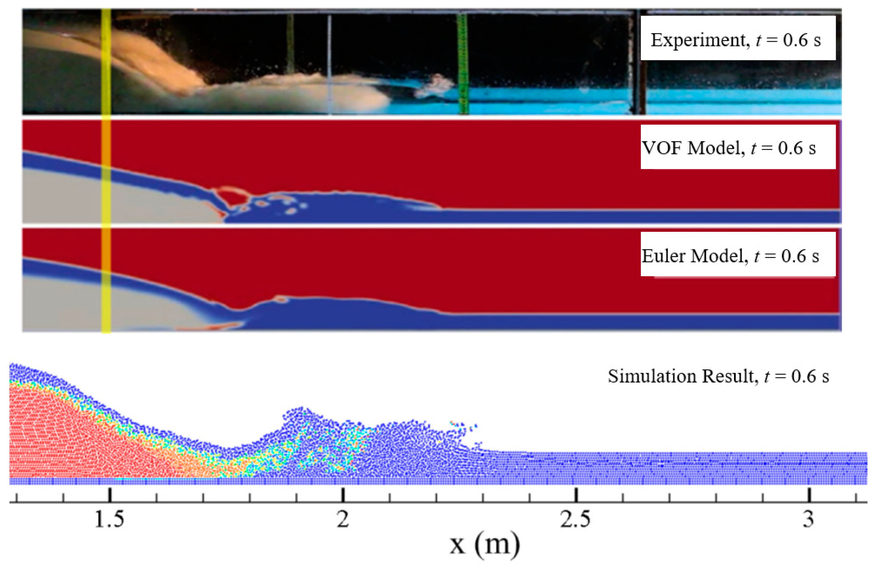
In this simulation, when t = 0.2 s, the clear water upstream touches the downstream stationary water surface and initiates the forward wave, which is consistent with the experimental results. When t = 0.6 s, the simulation results propagate to 2.3 m in the lateral direction (2.25 m for the tested results).

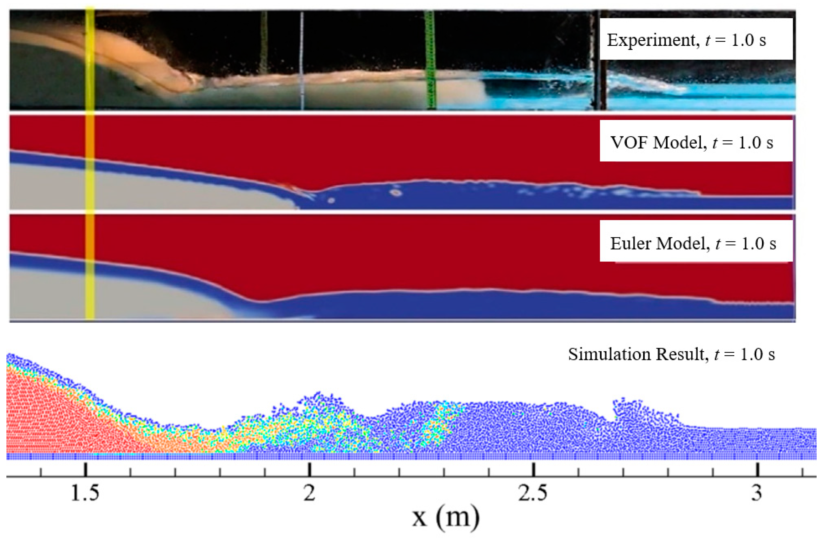
When t = 0.8 s and t = 1.0 s, the simulation results propagate to 2.6 m and 2.9 m in the lateral direction, and the test results propagate to 2.6 m and 2.85 m in the lateral direction. The simulated results are remarkably close to the experimental values, which proves that the model developed can accurately capture the wave propagation.

Vosoughi et al. [39] studied the process of dam break of a reservoir silting through experiments and obtained abundant experimental data by using high-speed cameras. In addition, they simulated the multi-phase flow problem involved in reservoirs silting by using the VOF method and the Euler method and obtained more accurate simulation results. The experimental results, the simulation results of the VOF method and the Euler method, and the simulation results of the model developed in this study are shown and visually compared in Figure 8.

As can be seen from Figure 8, when t = 1.0 s, all three mathematical models can obtain the forward wave propagation to the 2.9 m position. One advantage of the model developed in this study is that it can simulate the distance of water–sand mixing very well. The simulation results show that the water–sand mixing can reach 2.35 m, while in the experimental test it reaches 2.4 m; thus, the two results are remarkably close. Another advantage is considering the accurate replica of the simulation of the water fall, which agrees well with the experiment.

Furthermore, the sediment–water mixing and the wave propagation were predicted with the break of a reservoir silting, and the further development of the flow and siltation process were both simulated, and the results are shown in Figure 9 and Figure 10.

While the reservoir releases the water and sediments, the mixing increases while they both move downstream, and after t = 1.4 s, the mixed water and sand reach 2.6 m; when t = 1.8 s, the mixed water and sand are at 2.9 m. From Figure 9, it can be seen that at t = 2.2 s, t = 2.6 s, and t = 3 s, in the front section of the water–sand mixing, the main body has a part of the water–sand mixing particles, while at t = 3 s, this part of the particles spread as far as 4.2 m, and the sediment phase volume fraction of these water–sand mixing particles is negligible.

It can also be seen from the test results shown in Figure 9 that there is a part of the water body with a low degree of water and sand mixing. This water body section is between the front section with the clear water and the back section with a large concentration of water- sand mixing. This water body section is a transitional section. For the wave propagation, the forward wave propagates to 3.3 m when the dam break occurs at t = 1.4 s, and the wave propagates to 5.4 m when t = 3 s. (Figure 10)

5.3. Model Application III

Barrier dams are formed when rivers are blocked by earthquakes, rainstorm-induced landslides, cave-ins, mudslides, etc. Barrier dams have a loose structure and can collapse easily under the action of water scouring and erosion, resulting in the rapid discharge of copious amounts of stored water that can cause flood disasters and threaten the safety of people and buildings in the downstream area.

The Tangjiashan barrier dam induced by the Wenchuan earthquake in 2008 and the Baige barrier dam on the Jinsha River caused by a landslide in 2018 both seriously threatened the safety of cities downstream.

The barrier dam break mechanism is complex and difficult to predict, and multiple factors, such as its internal structure, geometry, compactness, and reservoir capacity, can affect the barrier dam break process. Therefore, the prediction of the barrier dam break process and the evolution of the break dam flood can help to assess the risk of the barrier dam to arrange for the timely evacuation of people. Barrier dams have two main forms of damage, seepage and diffuse topping, and according to the United States Geological Survey, 90% of barrier dam breaks are caused by diffuse topping [43].

In general, the length of a barrier dam along the river direction is much larger than the width of the dam perpendicular to the river direction, and it is necessary to focus on the changes along the river direction during the barrier dam break. Therefore, in this section, the established 2D water–sand two-phase flow model is applied to simulate the evolution of the diffuse topping out of a barrier dam. Considering that the barrier dam, once formed, will completely block the river, the initial state downstream of the barrier dam is set as a dry riverbed.

The initial setting of the barrier dam is shown in Figure 11. The initial water body and the barrier dam are kept stationary, the volume fraction of the sediment phase of the barrier dam at the initial moment is set to the uncompacted initial sediment volume fraction of 0.53, the barrier dam is 0.1 m high and 0.2 m long, the upstream water depth is 0.12 m, the total channel length is 1.8 m, and the channel slope is 2%. Because the water stored in the barrier dam is much larger than the upstream-supplying discharge, the upstream-supplying discharge is ignored when the barrier dam break process is simulated. The barrier dam break process and flow velocity distribution are shown in Figure 12 and Figure 13, respectively.

Figure 12 shows the volume fraction distribution of the sediment phase in the SPH particles after the barrier dam break. The change in the volume fraction of the sediment phase reflects the mixing degree and the mixing process of sediment and water. Compared with the initial downstream dam break in the presence of water simulated above in this section, the water–sand mixing caused by the barrier dam break is weaker in the absence of initial downstream water. Moreover, the water–sand mixing occurs near the water–sand interface, indicating that the erosion of the water flow during the barrier dam break is surface scouring. In contrast to the “steep hill” erosion of a homogeneous earthen dam, where the toe of the downstream slope gradually increases to form a “steep hill” and develops upstream, the crest elevation gradually decreases during barrier dam break, and the slope angle of the barrier dam along the flow direction gradually decreases.

The numerical results show that the barrier dam height decreases to 0.08 m after 0.5 s of the break, 0.06 m after 1.0 s of the break, 0.04 m after 2.0 s of the break, 0.03 m after 3.0 s of the break, and the maximum thickness of sediments accumulated on the riverbed is 0.01 m after 10 s of the break. At the initial stage, the barrier dam breaks quickly, and the barrier dam height decreases quickly; then, the decrease in the barrier dam height declines gradually, which is related to the stabilization of the geometry of the barrier dam after the barrier dam breaks. On the other hand, the reduction in the reservoir capacity of the barrier dam and the decrease in the flow velocity of the water at the top of the barrier dam leads to a decrease in the erosion capacity of the water. After the barrier dam breaks, there is basically no residual dam body, the water stored in the barrier dam is able to wash away the barrier dam, and the sand flows downstream completely with the water body. The sediment in the barrier dam silts up in the whole riverbed, and the deepest siltation does not occur in the initial position of the barrier dam, but in the middle section of the whole riverbed where the sediment is silted up.

Figure 14 shows the change of the water level in the reservoir over time. At 3 s after the dam break, the water level dropped to 0.06 m; 10 s after the dam break, the water level dropped to 0.03 m. After the dam break occurred, the water in the barrier dam was discharged rapidly, and the water level in the reservoir dropped quickly. From the slope of the curve, it can be seen that the decline rate of water level firstly in-creased and then decreased, so the surface flow velocity at the dam break site also changed accordingly. The velocity distribution after the barrier dam break is shown in Figure 13. It shows that the velocity of the surface flow at the break site firstly increased and then decreased, up to 1 m/s. Since there is no strong mixing of water and sand, the velocity of the upper layer of the flow is obviously larger than the velocity of the lower layer of sediment movement, and the velocity stratification is evident. As the water level in the barrier dam gradually decreases, the flow velocity gradually decreases and eventually tends to be close to the stationary water body.

Figure 15 shows an enlarged view of the flow field and the barrier of the barrier dam at the dam break site (center at x = 0.5 m). It can be seen that after the dam break, the velocity of the upper layer of flow is significantly larger than the velocity of the lower layer of sediment, and the sediment erosion mainly occurs at the water–sand interface, which again proves that the erosion of water flow as described above is mainly surface scouring. The flow velocity of the water moving from the top of the barrier dam can be clearly seen in the enlarged figure. After passing the highest point of the barrier dam, the velocity starts to increase. The position of the highest point of the barrier dam gradually moves downstream with the development of the dam break. Eventually, the barrier dam at the original break site can be completely washed away downstream.

6. Discussion

In this section, it is possible to find the application summary of the findings. The limitations of this study are highlighted considering the context of real-world engineering problems and the application of this work.

6.1. Summary of the Study

During the last decade, floods and natural disasters have become more severe and frequent due to population growth, climate change, deforestation, and changes in land use [44,45]. Dam breaks usually lead to significant damage to property and can cause loss of human life.

After a dam break occurs, it causes a complex water–sediment interaction that travels downstream, altering bed formation and impacting urbanized areas. This study aimed to build a computationally efficient hydrodynamic and sediment transport model for 2D dam break flows. Considering the two-phase flow characteristics and the water–sediment two-phase interaction exhibited by the sediment-containing water flow, this study converted Euler’s equations into Lagrangian’s equations based on the Eulerian control equation for turbulent mean two-phase flow, after which the equations were discretized into the form of particle summation using the SPH method, with one SPH particle representing two phases of water and sediment and each SPH particle carrying the physical information of the two phases. The model was first used for the simulation of the collapse process of a submerged accumulation body, and the accuracy of the model was verified. The reliability of the model performance was investigated by checking its ability to capture the typical phenomenon of the generation of the vortex behind the water body when the dam collapses. The results showed that this caused the suspension of the sediment, which started to move downstream.

In the application of the model, the water–sediment mixing process and the wave propagation process after the dam break were simulated and studied to predict each phase after the dam break. The previous experimental results found in the literature were adopted for comparison against the numerical ones. The SPH simulations were capable of replicating the following mechanisms:

-

The initial collapse;

-

The mixing of water and sediments released;

-

The flow velocity distribution of the upper flow layer, which is significantly larger than that of the lower sediment layer;

-

The flow velocities of the two layers when water and sediments are fully mixed.

6.2. Limitations of the Approach

The method developed in this research is based on the mixture theory and used to solve 2D problems. It describes the motion of water and sediment macroscopically in 2D using continuous media. However, this approach, in its current form, has certain limitations if it is used to simulate real-world engineering problems.

First of all, it is developed for 2D problems, while most of the engineering applications cannot be formulated in 2D due to the presence of 3D mechanisms in the flow and sediment motions. For example, the effect of the solid skeleton in the sediment media on the flow cannot always be represented in 2D and using continuous media in the macroscopic scale. It is probably more accurate to use microscopic discretization of the domain, preferably in the Direct Numerical Simulation (DNS) framework, to be able to resolve all the motion scales, or if not possible, in the LES framework to at least resolve 80% of the scales to have an adequate turbulence modeling process, as Pope [46] suggested. However, this is not easy to achieve due to the limitations of the current computational power and the complexity of the problems. Therefore, the idea is to use macroscopic modeling with a relatively rough discretization of the domain and tolerate a certain amount of error in the result of the model.

Even though the macroscopic approach provides a faster and less expensive modeling tool, the method is still not applicable to simulating large-scale sediment transport problems, e.g., in terrain, due to the requirement of discretizing large areas in the order of hundreds of meters or even kilometers. Therefore, for such a purpose, shallow-water forms of the equations need to be developed and tested, as those forms are suitable for large-scale applications where the variations of flow and sediment movement in the vertical direction can be neglected.

It is notable that the model applications in this paper have been set out to simulate cases where there were available existing experimental data and/or cases in which the model is capable of modeling, as discussed above. This was conducted in order to be able to test the performance of the model for sediment transport induced by dam break under flat and inclined bed conditions; however, the authors are fully aware that these may not represent all real-world applications that can be found.

7. Conclusions

A two-phase flow model was developed in the Lagrangian framework based on the mixture theory. The model was applied to solve 2D problems of dam break-induced sediment motion on a macroscopic scale. It was demonstrated that the model is capable of predicting preliminary wave propagations and bed evolution due to dam break, and the results, being promising and reliable, confirmed the capability of the SPH model, particularly for applications in the area of flood control and watershed management, although still not mature for practical use.

The limitations of the developed modeling framework were discussed in Section 6.2 in detail. They indicate the paths toward further development of the model to be applicable to real-world engineering problems. This has been considered by the authors as a possible pathway for future study.

References

1. Ivarson, M.M.; Trivedi, C.; Vereide, K. Investigations of Rake and Rib Structures in Sand Traps to Prevent Sediment Transport in Hydropower Plants. Energies 2021, 14, 3882. [Google Scholar] [CrossRef]
2. Morche, D.; Schmidt, K.H. Sediment transport in an alpine river before and after a dambreak flood event. Earth Surf. Process. Landf. 2011, 37, 347–353. [Google Scholar] [CrossRef]
3. Wang, G.; Tian, S.; Hu, B.; Xu, Z.; Chen, J.; Kong, X. Evolution Pattern of Tailings Flow from Dam Failure and the Buffering Effect of Debris Blocking Dams. Water 2019, 11, 2388. [Google Scholar] [CrossRef]
4. Xiong, J.; Tang, C.; Gong, L.; Chen, M.; Li, N.; Shi, Q.; Zhang, X.; Chang, M.; Li, M. How landslide sediments are transferred out of an alpine basin: Evidence from the epicentre of the Wenchuan earthquake. Catena 2022, 208, 105781. [Google Scholar] [CrossRef]
5. Quecedo, M.; Pastor, M.; Herreros, M.I. Numerical modelling of impulse wave generated by fast landslides. Int. J. Numer. Methods Eng. 2004, 59, 1633–1656. [Google Scholar] [CrossRef]
6. Hajigholizadeh, M.; Melesse, A.M.; Fuentes, H.R. Erosion and Sediment Transport Modelling in Shallow Waters: A Review on Approaches, Models and Applications. Int. J. Environ. Res. Public Health 2018, 15, 518. [Google Scholar] [CrossRef] [PubMed]
7. Sun, X.; Zhang, G.; Wang, J.; Li, C.; Wu, S.; Li, Y. Spatiotemporal variation of flash floods in the Hengduan Mountains region affected by rainfall properties and land use. Nat. Hazards 2022, 111, 465–488. [Google Scholar] [CrossRef]
8. Palu, M.C.; Yulien, P.Y. Modeling the Sediment Load of the Doce River after the Fundão Tailings Dam Collapse, Brazil. J. Hydraul. Eng. 2019, 145. [Google Scholar] [CrossRef]
9. Bosa, S.; Petti, M. A numerical model of the wave that overtopped the Vajont Dam in 1963. Water Resour. Manag. 2013, 27, 1763–1779. [Google Scholar] [CrossRef]
10. Gabreil, E.; Wu, H.; Chen, C.; Li, J.; Rubinato, M.; Zheng, X.; Shao, S. Three-dimensional smoothed particle hydrodynamics modeling of near-shore current flows over rough topographic surface. Front. Mar. Sci. 2022, 9, 935098. [Google Scholar]
11. Li, J.; Liu, H.; Gong, K.; Tan, S.K.; Shao, S. SPH modeling of solitary wave fissions over uneven bottoms. Coast. Eng. 2012, 60, 261–275. [Google Scholar] [CrossRef]
12. Shu, A.; Wang, S.; Rubinato, M.; Wang, M.; Qin, J.; Zhu, F. Numerical Modeling of Debris Flows Induced by Dam-Break Using the Smoothed Particle Hydrodynamics (SPH) Method. Appl. Sci. 2020, 10, 2954. [Google Scholar] [CrossRef]
13. Wang, S.; Shu, A.; Rubinato, M.; Wang, M.; Qin, J. Numerical Simulation of Non-Homogeneous Viscous Debris-Flows based on the Smoothed Particle Hydrodynamics (SPH) Method. Water 2019, 11, 2314. [Google Scholar] [CrossRef]
14. Zhang, Y.; Rubinato, M.; Kazemi, E.; Pu, J.H.; Huang, H.; Lin, P. Numerical and experimental analysis of shallow turbulent flows over complex roughness beds. Int. J. Comput. Fluid Dyn. 2019, 33, 202–221. [Google Scholar] [CrossRef]
15. Li, Z.; Dufour, F.; Darve, F. Modelling rainfall-induced mudflows using FEMLIP and a unified hydro-elasto-plastic model with solid-fluid transition. Eur. J. Environ. Civ. Eng. 2018, 22, 491–521. [Google Scholar] [CrossRef]
16. Jakob, M.; McDougall, S.; Weatherly, H.; Ripley, N. Debris-flow simulations on Cheekye River, British Columbia. Landslides 2013, 10, 685–699. [Google Scholar] [CrossRef]
17. Hirt, C.W.; Nichols, B.D. Volume of fluid (VOF) method for the dynamics of free boundaries. J. Comput. Phys. 1981, 39, 201–225. [Google Scholar] [CrossRef]
18. Sethian, J.A. Level Set Methods and Fast Marching Methods: Evolving Interfaces in Geometry Fluid Mechanics, Computer Vision and Materials Science; Cambridge University Press: Cambridge, UK, 2000. [Google Scholar]
19. Liu, G.R.; Liu, M.B.; Li, S. Smoothed particle hydrodynamics—A meshfree method. Comput. Mech. 2004, 33, 491. [Google Scholar] [CrossRef]
20. Vacondio, R.; Rogers, B.D.; Stansby, P.K.; Mignosa, P. SPH modeling of shallow flow with open boundaries for practical flood simulation. J. Hydraul. Eng. 2012, 138, 530–541. [Google Scholar] [CrossRef]
21. Shao, S.; Edmond, L.Y.M. Incompressible SPH method for simulating Newtonian and non-Newtonian flows with a free surface. Adv. Water Resour. 2003, 26, 787–800. [Google Scholar] [CrossRef]
22. Hosseini, S.M.; Manzari, M.T.; Hannani, S.K. A fully explicit three-step SPH algorithm for simulation of non-Newtonian fluid flow. Int. J. Numer. Methods Heat Fluid Flow 2007, 17, 715–735. [Google Scholar] [CrossRef]
23. Ran, Q.; Tong, J.; Shao, S.; Fu, X.; Xu, Y. Incompressible SPH scour model for movable bed dam break flows. Adv. Water Resour. 2015, 82, 39–50. [Google Scholar] [CrossRef]
24. Fourtakas, G.; Rogers, B.D. Modelling multi-phase liquid-sediment scour and resuspension induced by rapid flows using Smoothed Particle Hydrodynamics (SPH) accelerated with a Graphics Processing Unit (GPU). Adv. Water Resour. 2016, 92, 186–199. [Google Scholar] [CrossRef]
25. Bui, H.H.; Sako, K.; Fukagawa, R. Numerical simulation of soil–water interaction using smoothed particle hydrodynamics (SPH) method. J. Terramech. 2007, 44, 339–346. [Google Scholar] [CrossRef]
26. Pahar, G.; Dhar, A. Coupled incompressible Smoothed Particle Hydrodynamics model for continuum-based modelling sediment transport. Adv. Water Resour. 2017, 102, 84–98. [Google Scholar] [CrossRef]
27. Ulrich, C.; Leonardi, M.; Rung, T. Multi-physics SPH simulation of complex marine-engineering hydrodynamic problems. Ocean. Eng. 2013, 64, 109–121. [Google Scholar] [CrossRef]
28. Wang, D.; Li, S.; Arikawa, T.; Gen, H. ISPH simulation of scour behind seawall due to continuous tsunami overflow. Coast. Eng. J. 2016, 58, 1650014. [Google Scholar] [CrossRef]
29. Manenti, S.; Sibilla, S.; Gallati, M.; Agate, G. SPH simulation of sediment flushing induced by a rapid water flow. J. Hydraul. Eng. 2012, 138, 272–284. [Google Scholar] [CrossRef]
30. Shi, H.B. Two-phase flow models and their application to sediment transport. Ph.D. Thesis, Tsinghua University, Beijing, China, 2016. (In Chinese). [Google Scholar]
31. Shi, H.; Si, P.; Dong, P.; Dong, P.; Yu, X. A two-phase SPH model for massive sediment motion in free surface flows. Adv. Water Resour. 2019, 129, 80–98. [Google Scholar] [CrossRef]
32. Chauchat, J.; Cheng, Z.; Nagel, T.; Bonamy, C.; Hsu, T.J. SedFoam-2.0: A 3-D two-phase flow numerical model for sediment transport. Geosci. Model Dev. 2017, 10, 4367–4392. [Google Scholar] [CrossRef]
33. Lucy, L.B. A numerical approach to the testing of the fission hypothesis. Astrophys. J. 1977, 8, 1013–1024. [Google Scholar] [CrossRef]
34. Gingold, R.A.; Monaghan, J.J. Smoothed particle hydrodynamics: Theory and application to non-spherical stars. Mon. Not. R. Astron. Soc. 1977, 181, 375–389. [Google Scholar] [CrossRef]
35. Monaghan, J.J. Simulating free surface flows with SPH. J. Comput. Phys. 1994, 110, 399–406. [Google Scholar] [CrossRef]
36. Monaghan, J.J.; Kos, A. Solitary waves on a Cretan Beach. J. Waterw. Port Coast. Ocean. Eng. 1999, 125, 145–155. [Google Scholar] [CrossRef]
37. Monaghan, J.J. Smoothed Particle Hydrodynamics. Annu. Rev. Astron. Astrophys. 1992, 30, 543–574. [Google Scholar] [CrossRef]
38. Kazemi, E.; Koll, K.; Tait, S.; Shao, S. SPH modelling of turbulent open channel flow over and within natural gravel beds with rough interfacial boundaries. Adv. Water Resour. 2020, 140, 103557. [Google Scholar] [CrossRef]
39. Vosoughi, F.; Rakhshandehroo, G.R.; Nikoo, M.R.; Sadegh, M. Experimental study and numerical verification of silted-up dam break. J. Hydrol. 2020, 590, 125267. [Google Scholar] [CrossRef]
40. Wang, C.; Wang, Y.; Peng, C.; Meng, X. Two-fluid smoothed particle hydrodynamics simulation of submerged granular column collapse. Mech. Res. Commun. 2017, 79, 15–23. [Google Scholar] [CrossRef]
41. Rondon, L.; Pouliquen, O.; Aussillous, P. Granular collapse in a fluid: Role of the initial volume fraction. Phys. Fluids 2011, 23, 73301. [Google Scholar] [CrossRef]
42. Wang, C.; Wang, Y.; Peng, C.; Meng, X. Dilatancy and compaction effects on the submerged granular column collapse. Phys. Fluids 2017, 29, 103307. [Google Scholar] [CrossRef]
43. Costa, J.E.; Schuster, R.L. The formation and failure of natural dams. Geol. Soc. Am. Bull. 1988, 100, 1054–1068. [Google Scholar] [CrossRef]
44. Rubinato, M.; Luo, M.; Zheng, X.; Pu, J.H.; Shao, S. Advances in Modelling and Prediction on the Impact of Human Activities and Extreme Events on Environments. Water 2020, 12, 1768. [Google Scholar] [CrossRef]
45. Rubinato, M.; Nichols, A.; Peng, Y.; Zhang, J.; Lashford, C.; Cai, Y.; Lin, P.; Tait, S. Urban and river flooding: Comparison of flood risk management approaches in the UK and China and an assessment of future knowledge needs. Water Sci. Eng. 2019, 12, 274–283. [Google Scholar] [CrossRef]
46. Pope, S.B. Turbulent Flows; Cambridge University Press: Cambridge, UK, 2000. [Google Scholar]
Figure 1. Example of flash flood: overview of the affected areas.
Water 15 03033 g001
Figure 2. Schematic diagram of the collapse of the accumulation body in still water.
Water 15 03033 g002
Figure 3. Simulation results of the collapse process of the accumulation body.
Water 15 03033 g003
Figure 4. Validation of accumulation body collapse process [42].
Water 15 03033 g004
Figure 5. Diagram of dam break of a reservoir silting.
Water 15 03033 g005
Figure 6. Simulation results of a dam break of a reservoir silting (sediment phase volume fraction map).
Water 15 03033 g006aWater 15 03033 g006b
Figure 7. Simulation results of a dam break of a reservoir silting (flow velocity distribution map).
Water 15 03033 g007aWater 15 03033 g007b
Figure 8. Dam break validation results of a reservoir silting (experiment, VOF model, and Euler model results from literature Vosoughi et al. [39]). Adapted with permission from Elsevier, Journal of Hydrology, License ID 1383966-1.
Water 15 03033 g008aWater 15 03033 g008b
Figure 9. Propagation of the sediment distribution after the dam break of a reservoir silting.
Water 15 03033 g009aWater 15 03033 g009b
Figure 10. Flow velocity distribution during the dam break phenomenon of a reservoir silting.
Water 15 03033 g010aWater 15 03033 g010b
Figure 11. Schematic diagram of the initial state of the barrier dam break.
Water 15 03033 g011
Figure 12. Sediment volume fraction distribution after the barrier dam break.
Water 15 03033 g012aWater 15 03033 g012b
Figure 13. Flow velocity distribution after the barrier dam break.
Water 15 03033 g013aWater 15 03033 g013b
Figure 14. The process of reservoir water level change after the barrier dam break.
Water 15 03033 g014
Figure 15. Enlarged view of the flow field at the barrier dam break site.
Water 15 03033 g015aWater 15 03033 g015b
Disclaimer/Publisher’s Note: The statements, opinions and data contained in all publications are solely those of the individual author(s) and contributor(s) and not of MDPI and/or the editor(s). MDPI and/or the editor(s) disclaim responsibility for any injury to people or property resulting from any ideas, methods, instructions or products referred to in the content.