Investigation of Water Dynamics Nearby Hydroelectric Power Plant of the Gorky Reservoir on Water Environment: Case Study of 2022

Abstract

Regulated water bodies like lakes and reservoirs are increasingly becoming an object of attention due to the problems of greenhouse gas emissions, regional ecology, and the necessity to ensure safe environmental management. However, for some local tasks, it is important to assess the contribution of a hydroelectric power plant (HPP) to various parameters of the nearest water environment, for example, mortality of zooplankton, transfer of suspended matter and phytoplankton, formation of secondary deposits, methane emissions, spatial features of stratification, etc. An example of such studies is the present paper. It is based on unique data of complex measurements of hydrophysical, hydrooptical, hydrobiological, and hydrochemical water parameters, as well as methane fluxes, that were collected at the Gorky Reservoir nearby a HPP in the spring, summer, and autumn of 2022. Preliminary correlations between these parameters were obtained. The results are useful for the correct interpretation of satellite images of inland waters, quantitative description of HPPs’ influence on the water environment, knowledge of the main patterns of transformation of aquatic organism communities under conditions of runoff regulation, determination of water quality by hydrobiological parameters, development of mechanisms for improving the ecological state of water bodies, and accounting spatial heterogeneity of methane flows from the surface of the reservoir.

1. Introduction

The regulation of river flow, accompanied by the creation of reservoirs, often serves as a necessary measure to ensure navigation, hydropower, various sectors of the economy, and safety [1,2,3,4,5]. The backside of this process is a gradual change in the hydrological, hydrooptical, hydrobiological, and hydrochemical properties of water and the growth of secondary soils. Usually, monitoring of key water properties is carried out on a grid of hydrological stations since the moment of a reservoir’s creation, but in the last decade, satellite data of high and medium resolutions have been actively used to cover large water areas. This makes it possible to estimate the influence of reservoirs on green gas exchange [6,7,8,9], regional climate [10,11], flora and fauna [12,13,14,15], etc. At the same time, the question of the influence of hydroelectric power plants (HPPs) on the nearest water environment remains poorly studied. There are no specialized or regular studies on this topic in the literature, which is probably due to the lower importance of this issue compared to those mentioned above, as well as locality and regionality. But for some water bodies and applications, such studies are extremely important.

The triggers for this study were the results of long-term field observations of hydrophysical processes as well as in situ measurements of water color and impurity concentrations under the satellite overpasses in the Gorky Reservoir, which often indicated a discrepancy in the measurement and satellite data within one day even in calm weather conditions [16,17]. A preliminary analysis of these discrepancies indicated the peculiarities of current, caused primarily by the variable volume of water discharge through a hydroelectric power plant.

Figure 1 presents the location of the Gorky Reservoir and a general view of its lake part. In general, the Gorky Reservoir is a part of a cascade of 10 reservoirs on one of the longest rivers in Russia—the Volga River. The last 100 km forms a lake part, ending with a dam and a hydroelectric power plant.

After the launch of the Gorky HPP in 1961, systematic monitoring of the water current was performed at the reservoir using buoy stations and float recorders [18]. Monographs [19] describe the averaged current and note their significant variability under the influence of two main factors: the runoff regulation by hydroelectric power plants and wind forcing. Since the Gorky Reservoir belongs to water bodies with high flow and seasonal regulation of runoff (water exchange coefficient is 5.41 [5]), essential seasonal variability of currents is regularly observed in the lake part. The current determined by the water discharge through the HPP prevails in winter. The same situation is observed in summer in conditions of calm weather. In the summer–autumn period, the water discharge is small (about 10% of the maximum discharge); therefore, wind-induced current and surge current prevail. As a result, the current remains predominant throughout the year in the old channel of the Volga, but wind-induced current plays the main role in the floodplain [19]. In a recently published paper [20], the newest detailed maps of current obtained for the lake part of the reservoir as a result of ship measurements using an acoustic Doppler current profiler (ADCP) were presented for two average daily discharges close to typical for the summer season. The authors found that even with a difference of 30% in water discharge, the current changes noticeably. In contrast to the open water areas of the seas and oceans, the structure of currents in inland waters with regulated flow is more complex. There are two types of circulation currents: classical vortexes associated with wind forcing and whirlpools, mainly determined by uneven runoff, coastline shape, and bathymetry [21].

But if we consider the area nearest to the HPP water (Figure 2), the situation is still significantly more complicated due to a faster response of the environment to the changed flow rate through the HPP (water discharge). According to [17], every day around noon, the water discharge increases significantly, by 2–3 times. This leads to an increase in the current velocity of the upper water layer and also contributes to the removal of well-heated and phytoplankton-rich waters from tributaries to the reservoir. This dynamic radically affects the accuracy of solving such urgent problems as satellite monitoring of hydrophysical processes and water quality [16,17,21,22]. In particular, according to [17], the overpass moments determined by all available satellite ocean color sensors lie between 10:00 a.m. and 12:00 p.m. local time (UTC + 3) and coincide with the peak value of the water discharge. At the same time, based on the analysis of in situ measurements of the current velocity on long transects with nearby HPPs, it was found that the manifestation of a daily increased water discharge can be observed on a scale of 1–2 h. As a result, the shape and position of foam bands and slicks or distribution of phytoplankton in the upper water layer can differ significantly from those previously registered by a satellite ocean color sensor.

In addition to the redistribution of substances and particles dissolved and suspended in water, HPPs also have a mechanical effect on them when water passes through turbines. This is especially true for zooplankton [23,24]. The causes and mechanisms that determine the dynamics of the quantitative indicators of zooplankton development are usually associated with birth and growth rates, without paying attention to mortality. Knowledge of natural mortality not associated with predation is the main tool for predicting and managing the state of aquatic ecosystems [25]. Therefore, such a study for hydro-biocenoses near HPPs seems to be relevant.

Variable hydrodynamic processes are also manifested in the origin and formation of the soil complex [26]. They determine changes in macrozoobenthos communities, and the bottom current velocity is one of the main factors determining the quantitative characteristics of benthos [27].

In addition to the above-described, the contribution of HPPs’ functioning on methane degassing from the reservoir bottom when compiling the balance of methane in reservoirs is known and actively studied, for example, in [28]. However, the effect of HPPs on methane flows upstream of dams in the zone of operation of hydraulic structures has not been practically studied. It is noted that high speeds during water releases through dams contribute to the washing out of fine sediments [29].

The preliminary results listed above emphasize the necessity for a more comprehensive look at the problem of HPPs’ impact on the water environment. To do this, in 2022, synchronized measurements of hydrophysical, hydrooptical, hydrobiological, and hydrochemical parameters, as well as concentrations and fluxes of greenhouse gases, were carried out downstream and upstream of the HPP of the Gorky Reservoir. The results of these studies are presented in this publication.

2. Materials and Methods

2.1. Study Area

The study area was defined as the lake part of the Gorky Reservoir with a nearby HPP (Figure 2). This area includes the Volga channel, tributaries of three rivers along the right bank (Yug, Trotsa, Sanahta), and a floodplain along the left bank. The average depth of the channel in this area is 18–24 m and 6–10 m for the floodplain.

Figure 2 shows a map of three transects (AB, AC, EF) and stations in the upstream and downstream areas superimposed on the bathymetry. The regular set of stations consisted of 5 stations in the upstream area and 5 stations in the downstream one, mirrored relative to the dam. Upstream station #1 (U1) and downstream station #1 (D1) were located 300 m upstream and downstream of the intake on the Volga River channel, respectively. Other stations (stations U2-4 and D2-4) were selected to the left of the channel along the dam to assess the variability of measured characteristics depending on the distance from the HPP entrance. Irregular stations (U6-U14) covered both channel and floodplain parts of the reservoir, as well as tributaries, to trace the boundary of the HPP’s influence on investigated parameters.

Complex measurements at the regular stations were carried out three times: in spring (25 May 2022–26 May 2022), in summer (8 August 2022), and in autumn (12 October 2022). Due to the impossibility to combine all teams on one day, water and soil sampling and measurements of methane concentrations and fluxes in August were shifted to 24 August 2022–25 August 2022 (instead of 8 August 2022). Measurements of current parameters were carried out on mentioned dates and an 2–3 additional times each month.

In the upstream area, measurements were carried out from two vessels. The first vessel, the floating hydrophysical laboratory “Geophysicist”, was used for continuous recording of current and wind parameters. The high-speed motorboat “Volzhanka-46” was used for rapid movement between stations for water and soil sampling and sounding. In the downstream area (below the HPP) all works were carried out from a motorboat.

2.2. HPP Operation Mode

Data on HPP discharge with 1 h discreteness were provided by the operational company RusHydro in the form of the table “date/time/water discharge (m³/s)”. The averaged data on daily discharge are available in the public domain [30].

2.3. Field and Laboratory Measurements

2.3.1. Meteorology

Wind speed and direction measurements continuously recorded from onboard the Geophysicist using a WindSonic digital ultrasonic anemometer with a frequency of 4 Hz were automatically converted to true wind with vessel course and speed and recalculated to a 10 m horizon. These data were used for wind drift correction. Other meteorological parameters (e.g., wind or precipitation on previous days) were downloaded from open meteorological data sources [31] or determined in situ by a Kestrel hand-held weather station.

2.3.2. Hydrophysical Parameters

Currents were measured continuously along the vessel’s course using a WorkHorse Monitor 1200 kHz acoustic Doppler current profiler (ADCP) with a frequency of 1 Hz. The resolution of the depth was 0.5 m, starting from the first horizon of 0.6 m. Hydrophysical measurements at the stations included measurements of vertical profiles of temperature and conductivity, dissolved oxygen, pH, turbidity, chlorophyll a, and dissolved organic matter concentrations were performed using a YSI Pro30 conductometer, a YSI ProODO oximeter and a YSI Exo 3 multiparameter water quality sonde.

2.3.3. Hydrobiological Parameters

(a)

Phytoplankton

We collected integrated phytoplankton water samples from the total thickness of the photic zone (the photic zone being the double transparency estimated with a Secchi disk) and also ones from the surface horizon separately at each station. Integrated phytoplankton samples were collected with the help of a Ruttner water sampler (2 L) and preserved with an iodine–formaldehyde solution. During the collection of integrated samples, water was taken at equal-depth intervals, and equal volumes of sub-samples were mixed into one. Phytoplankton species identification was performed under a MEIJI Techno optical microscope (Saitama, Japan) with an oil immersion objective at magnifications of 200, 400, and 1000×. A list of guides used for species identification and a description of methods for concentrating phytoplankton samples were sourced from the paper [32]. The current taxa names were verified using the AlgaeBase website (algaebase.org, accessed on 19 June 2023) [33].

The authors analyzed such parameters of the phytoplankton communities as abundance (N (10⁶ cells/L)) and biomass (g/m³). A detailed description of the calculation of the indicators mentioned above is available in the work [34]. The dominant species included species with an abundance or biomass of more than 10% of the total value [35].

(b)

Zooplankton

To assess the natural level of injury/mortality of zooplankton organisms in the upstream area and their passage to the downstream one through the HPP, all zooplankton samples were stained with water-soluble aniline blue dye for 15 min, followed by fixation with concentrated formalin (40%) at the rate of its concentration in the sample, 10% [36]. Zooplankton samples were stained immediately after sampling on board. The cameral processing of the material was carried out according to generally accepted standard methods used in hydrobiological studies. Keys and manuals were used to identify zooplankton species. The number of species of planktonic organisms was counted and the average size of individuals of each species was determined by developmental stages. According to methodological recommendations [36], completely and almost completely (more than 2/3 of the body) colored (blue) organisms were taken into account as dead zooplankters. The proportion of the number or biomass of dead individuals of rotifers (Rotifera) and lower crayfish (Cladocera, Copepoda) from the total number or biomass of all zooplankton was used as an indicator of mortality. To assess the species structure of cenosis, the Kovnatsky–Paliy dominance index was used.

2.3.4. Hydrochemical Indicators

Hydrochemical analysis of surface samples was carried out using a V-1100 spectrophotometer, a «CAPEL 105 M» capillary electrophoresis system, a PRODIGY inductively coupled plasma atomic emission spectrometer (ICP spectrometer), and an HI 98130 water analyzer. Chemical analysis was performed in the laboratory of the Shared Use Center of the Institute of Chemistry, Lobachevsky University, Nizhny Novgorod, Russia. The measured parameters included the following indicators: iron, magnesium, calcium, phosphorus, chlorides, nitrites, sulfates, nitrates, phosphates, ammonium ions, bicarbonates, pH, and total mineralization.

2.3.5. Bottom Sediments

The organic matter (OM) content in the bottom sediments (BS) was estimated by weight loss during calcination. The work also included experiments to determine the fluxes of substances at the water–bottom sediment border using the tube method [37,38,39,40]. BS samples were collected with an Ekman–Berge dredge. A glass tube with a diameter of 3.5 cm and a height of 45 cm was inserted into the extracted core to collect the sample. The tube was filled under the plug with water from the bottom horizon taken at the station simultaneously with the BS sampling. The same water was also used to fill a “blank” tube without silt. All tubes were placed in dark bags and exposed at a temperature close to the bottom water temperature at the moment of sampling. Then, water from the tubes was drained by siphon and in it were determined dissolved oxygen, methane, phosphorus, and HCO₃⁻. Substance fluxes from 1 m² of bottom area per day were determined by the difference in substance concentrations in the tube with sediments and the blank tube. Total organic matter degradation in BS was determined by the amount of HCO₃⁻ released by the BS column during the exposure time, and aerobic degradation of OM in BS was estimated by the value of oxygen uptake by the core column.

2.3.6. Concentrations and Fluxes of Methane

The specific flux from the water to the atmosphere was determined by the “floating chamber” method [41]. Sealed plastic chambers with floats were exposed on the water’s surface for 30–60 min. A syringe was used to draw air from the chamber at the beginning and at the end of the exposure time into 20 mL vials pre-filled in the laboratory with a saturated NaCl solution. The values of specific methane flux were determined by the difference in methane concentration in the chamber at the beginning and at the end of the experiment; the volume of the above-water part of the chamber and the area of the water surface under it were known from the tare data. Determination of methane content in water was carried out by the “headspace” method [42]. Water samples of volume 40 mL from the Rutner bathometer were pumped into a syringe. Then, 20 mL of air was taken into the syringe and the syringe was shaken vigorously for 2–3 min to bring dissolved methane into equilibrium with the gaseous phase. An amount of 20 mL of air from the syringe was pumped into a vial with a NaCl solution, as in the method of air sampling from the chambers described above. To account for the methane content of the air, an air sample was taken separately at each measurement station where water was sampled for methane content.

A Chromatek Crystal 5000.2 gas chromatograph with a flame ionization detector was used to determine the methane concentration in the resulting samples. Determination of methane content in each sample was carried out in triplicate.

2.3.7. Statistical Analysis

As data did not have normal distribution, the non-parametrical Spearman correlation (Rs) was used to estimate the relationship between the environmental parameters and both abundance and biomass of phytoplankton groups. Statistical processing was conducted using the Statistica 10.0 software package (Statsoft TIBCO, Palo Alto, CA, USA). The authors discussed reliable connections of parameters at the significance level of p ≤ 0.05.

3. Results and Discussion

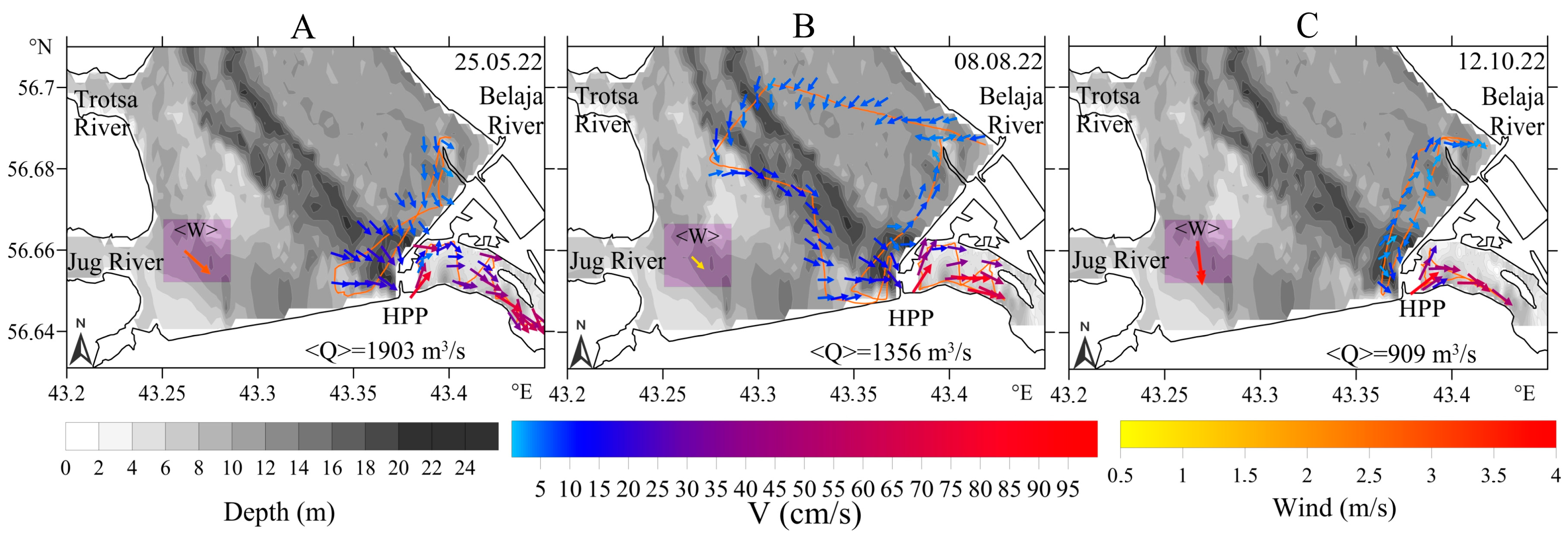
3.1. Multi-Scale Variations in Water Discharge

One of the main factors responsible for the variability of currents in the upstream section of the reservoir is the significant changes in the water discharge through the HPP. We have not encountered relevant information in the literature, so we consider it necessary to provide it not only for the year 2022 but also for the previous years, namely 2018–2021. This allows us to form a representation of all multi-scale variations. Figure 3 demonstrates the within-year variations in water discharge Q (m³/s) for 2018–2022 using open data [30]. It can be seen that every year, the HPP regime is unique up to mid-July. The winter of 2019 is especially notable due to the lowest discharge, not exceeding the summer low flow discharge. The prolonged spring peaks took place from early April to late May as usual, except in the year 2020 due to an early warm spring and peak discharges began in early March. The summer regime with a quasi-constant average daily flow rate of 1250 m³/s was observed for all years from mid-June and persisted until the end of August. The autumn flow regime depended on precipitation. Thus, in 2018, 2021, and 2022, water discharges were maintained until the end of the year at the summer level, but with noticeable fluctuations at 30% on average, while in 2019 and 2020, increased discharges (from 1.5 to 4 times) were first observed in the first autumn months, occurring until the end of the year.

The combination of inflow and discharge leads to a sharp rise in water level at the beginning of the annual spring flood. After this time, the water level stays near the normal background level and gradually decreases in June, staying stable until mid-December [30].

For this study, the ice-free period from May to October is the most important. Except for the beginning and end of this period in 2020 and 2022, the average daily water discharge during this period was at a quasi-constant level, approximately the same for all years under consideration, but had different fluctuations. These are explained by Figure 4, which presents a graph of water discharge with 1 h discretization for the ice-free period of 2022. It can be seen that water discharge during the interval under consideration is periodic and represents a sequence of pulses. The maximum discharge occurs at about 11:00 a.m. local time, the minimum one at midnight. Absolute values of maximum discharges are significantly higher after the May flood. From mid-June to mid-autumn, the daily discharge becomes stable with a minimum value of 900 m³/s and a peak value of 2400 m³/s. Based on this conclusion, it would seem that the distribution of currents on the reservoir should correlate with a periodic intensification of discharges and have a daily recurrence. However, in practice, such regularity is not observed, which is probably due to wind influence. In the next section, we considered the currents at different horizons separately in calm and windy weather and also constructed statistically averaged currents and calculated their variations.

3.2. Hydrophysical Parameters

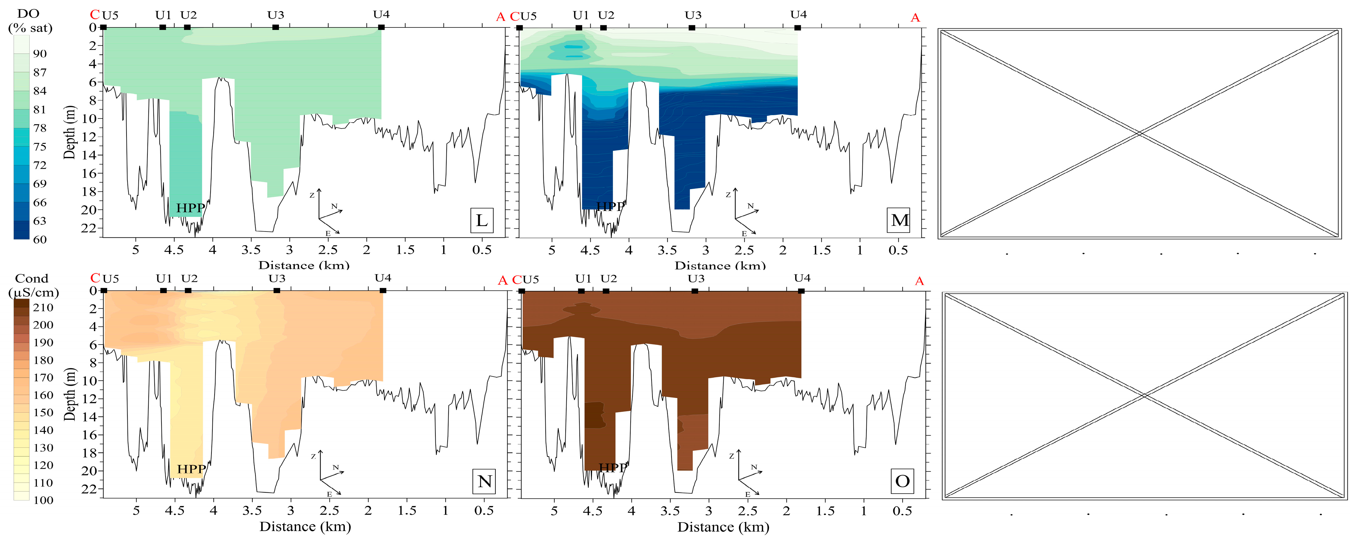
3.2.1. Upstream Area

The distribution of hydrophysical parameters strongly depends on the current, which, in addition to wind drift, is also determined by the variable water discharge through the hydroelectric power plant. Figure 5, Figure 6, Figure 7 and Figure 8 demonstrate this influence. Figure 5 shows the vector fields of currents at the horizon of 0.6 m in the upper and lower water horizons, where <W> is the average magnitude of wind speed for the period of the experiments and <Q> is the average daily water discharge. From Figure 5, it can be seen that in May, with a large daily discharge of 3520 m³/s, the upstream current is structured and directed towards the HPP; its velocity is about 20 cm/s over the channel and 5–7 cm/s over the floodplain. In August, with a noticeably lower discharge of 2260 m³/s, the current characteristics over the channel are close to those of May, but a whirlpool with a scale of several km and a speed increased to 10–12 cm/s is observed over the floodplain. At the lowest discharge in October (900 m³/s), the currents are similar to currents in August, but there is no noticeable intensification of the channel flow: the current velocities over the channel and floodplain are close, about 5–10 cm/s.

The vertical structure of the currents on the AC transect (Figure 2) of the upstream area is shown in Figure 6. The origin of the transect is taken as the point of departure from the channel (A). An interval of 4–4.7 km corresponds to the entrance channel of the HPP (station U1) and the idle discharge channel (station U2). The neighboring deep-water arm between 2.7–3.7 km (station U3) rests against the dam. Current velocity components in the transect–vertical plane are shown with arrows, and the colored background indicates velocity components perpendicular to the transect–vertical plane (the negative component is directed towards the HPP, positive—from the HPP to the north). It can be seen that in May, the whole water flow is formed near the Volga channel and has a constant vertical velocity of 25 cm/s. Below the depth of 16 m, velocity increases to 35–40 cm/s due to the entrance channel of the HPP. The lower layers in the floodplain move away from the Volga channel with minimal velocity. In August, with a typical average daily water flow of 1300 m³/s, the water velocity over the channel is also constant with depth but has lower absolute values (20 cm/s). However, the picture above the floodplain is completely different: the water layer is directed away from the channel and bends northward from the dam (positive velocity values in the range of 0–1.5 km), which is in good agreement with the spatial distribution of the current velocity in Figure 5B. The obtained data indicate that water circulation is formed near the left bank, and this occurs at some “optimal” water discharge (not too small and not too large, i.e., when the entire water column is carried away to the discharge point). Maybe the frequency of discharges also plays a role in circulation formation.

In October, with a minimum water discharge of 900 m³/s, the current velocity over the channel decreases to 10 cm/s, the velocity near the entrance channel of the HPP reaches 15 cm/s, and there is no pronounced current over the floodplain.

The binding of parameters measured by the sonde to the current variations is not obvious (Figure 6). At the same time, significant variations are visible between spring and summer measurements and in space. The stratification of the water column, bottom sediments, the distribution of phytoplankton and benthos, and the specific flow of methane have pronounced heterogeneity.

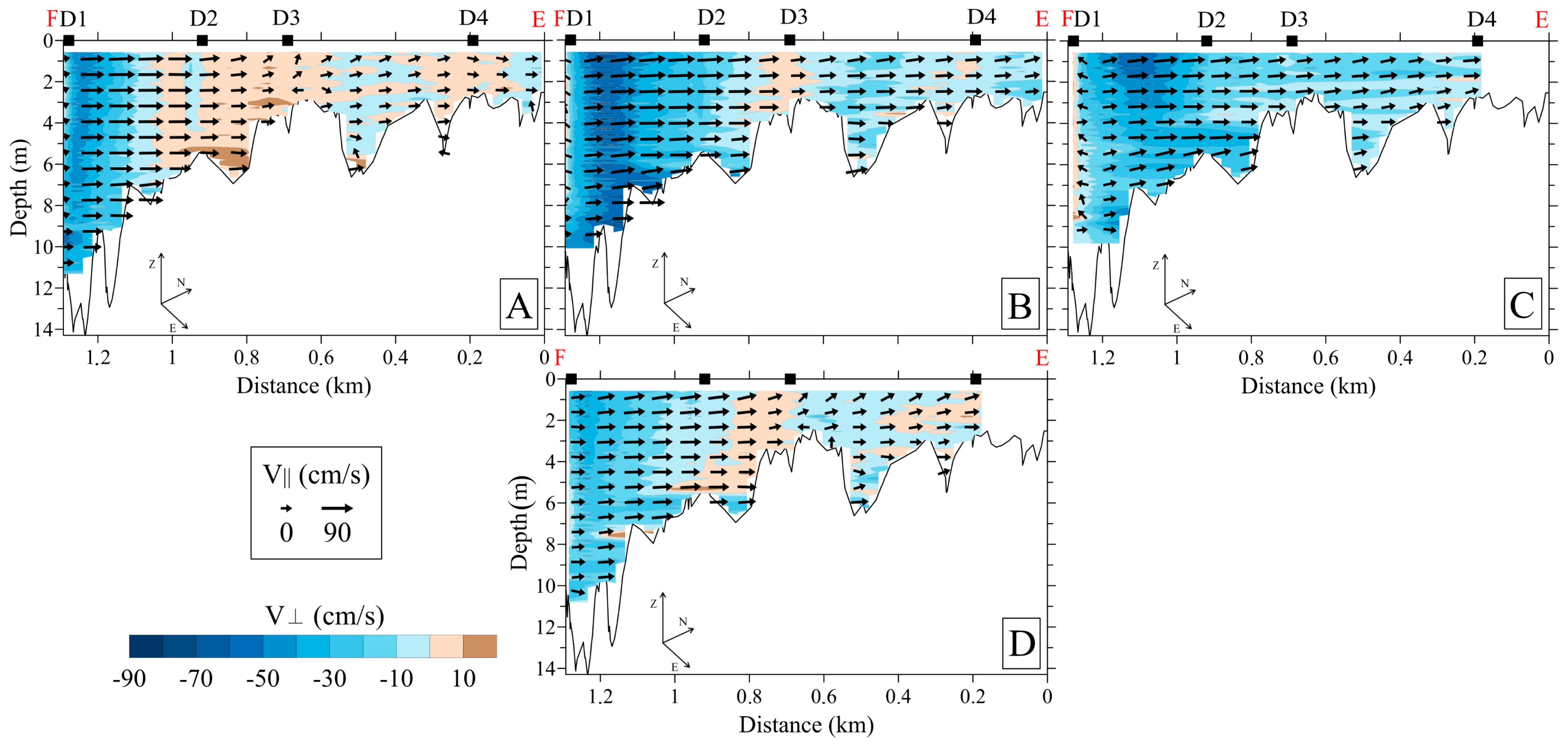
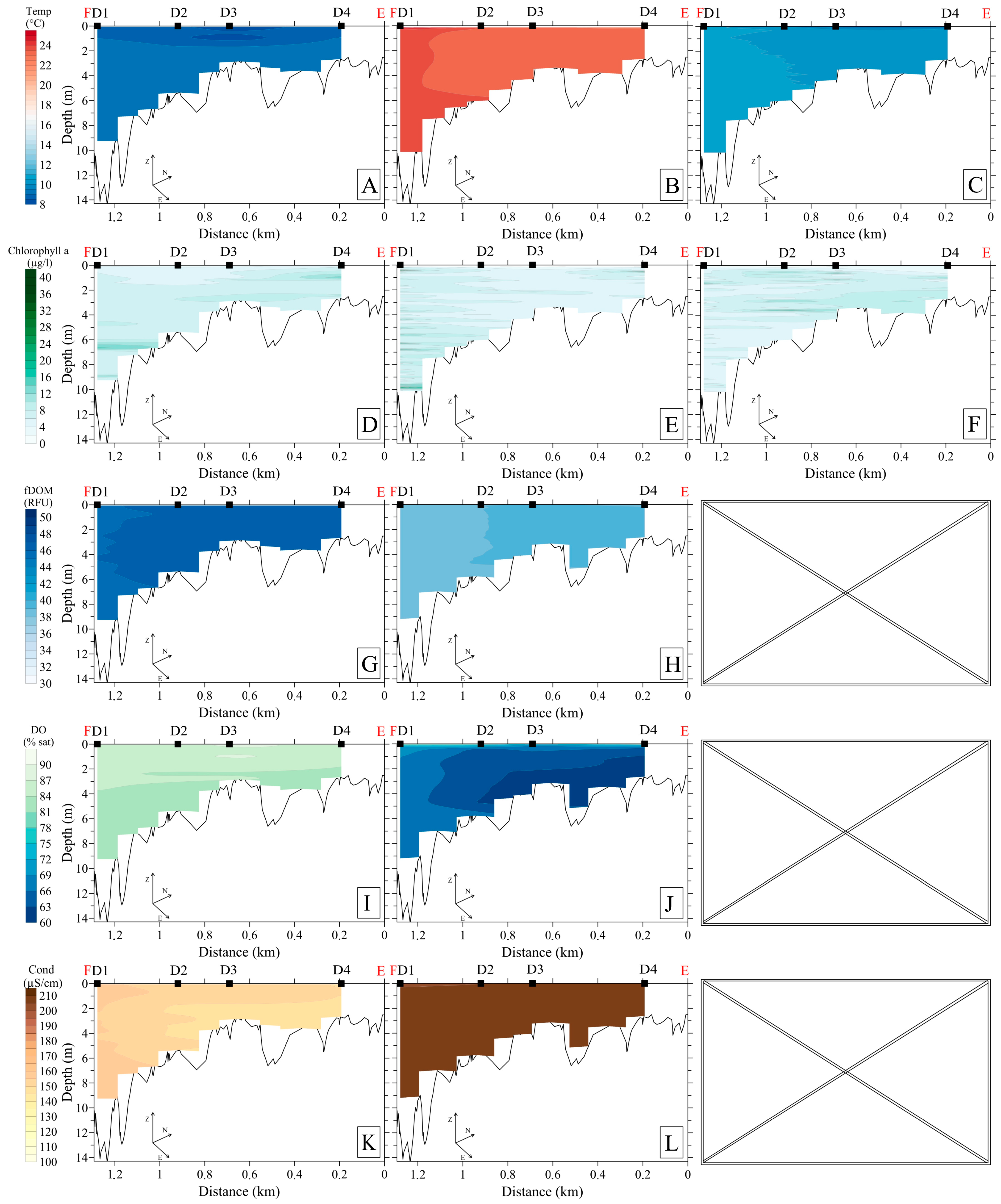
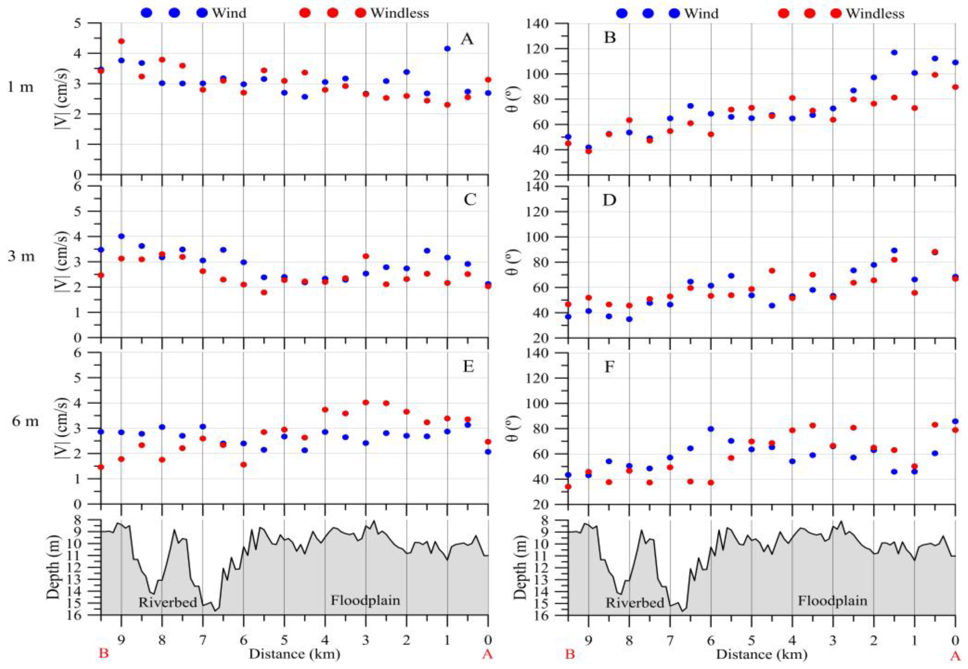
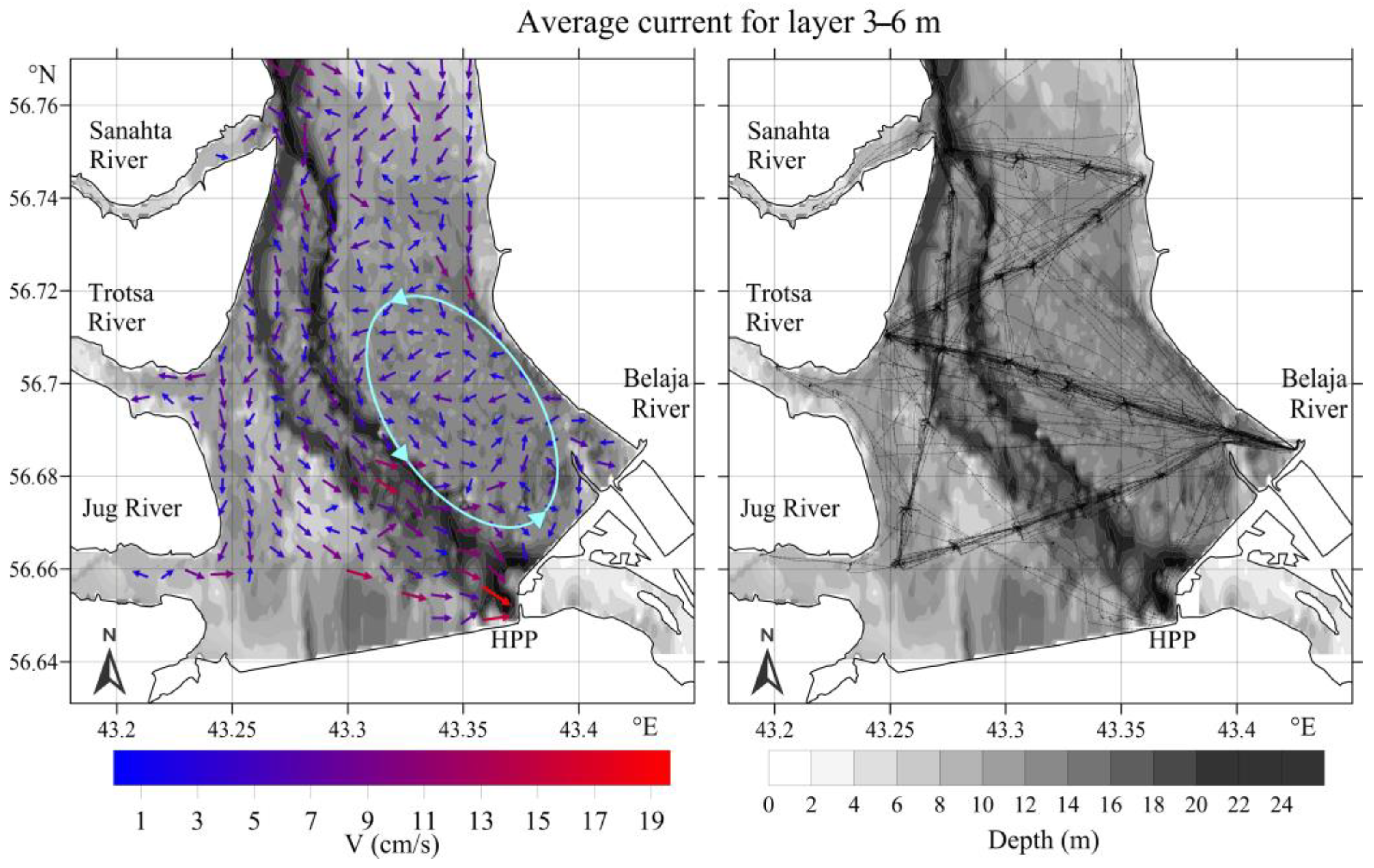
3.2.2. Downstream Area

In May, under the main water entrance channel of the HPP (station D1), the current is directed strictly perpendicular to the dam with a velocity rate from 0.1–0.5 m/s in the upper layer of 0–4 m and up to 1 m/s below (Figure 7, left). Slightly to the left (about 100 m, which is comparable to the length of the entrance channel), the current acquires a perpendicular velocity component with a magnitude of up to 1 m/s, i.e., equal to the longitudinal velocity component. Further to the left (between stations D2 and D3), the stream continues to bend towards the HPP, maintaining this direction to the left (station D4) over the floodplain. At the same time, the magnitude is significantly reduced to 10 cm/s, and the current becomes uniform in depth. In August (Figure 7, in the center), the picture is similar, with the difference that the idle discharge area is usually completely blocked due to the low water level in the reservoir. Probably for this reason, the main river current is slightly shifted to the left (by 100 m), clearly traced throughout the depth, but expanded while maintaining the same speed. The current over the floodplain is similar to that of the previous case. The displacement of and increase in the channel flow, as well as the strengthening of the perpendicular component, can also be associated with a decrease in current through part of the turbines located between stations D1 and D2. In May, measurements were carried out in the downstream area after the daily peak discharge, which may be accompanied by a partial overlap of turbines. In August, the measurements were carried out close to the daily peak of discharge, when, probably, the flow in all turbines decreased evenly. The structure of currents in the downstream area in May is similar to the structure of currents in August, measured at a later time with a lower discharge (Figure 7, bottom row). With minimal discharge in autumn (Figure 7, right), the current also retains the channel component, but at a lower speed (up to 1 m/s in the upper layer of 0–3 m, and up to 60 cm/s below). There is an increase in the flow of up to 20 cm/s over the floodplain. Downstream at a distance of 4 km, the channel flow retains its severity and significant speed up to 1 m/s (station D5).

The identified features of the flow dynamics are reflected in the distribution of some hydro-ecological characteristics (Figure 8). Compared to upstream, downstream of the dam, the water column is well mixed and transverse differences in water temperature and dissolved organic matter are not pronounced. In spring, the water conductivity has its minimum value in the stream upstream of the dam and, in summer, there is a weak vertical stratification. In the downstream section, transverse differences are not significant. Of all the measured characteristics, the distribution of dissolved oxygen is most contrasting in summer, when its content in the near-dam area (U1, U2) in the bottom layers decreases by 40% and this oxygen-depleted water mass is discharged downstream. The lowest values are observed at stations D3 and D4 along the back part of the dam body, where flow and aeration are reduced during discharges.

The presented results demonstrate current variations in relation to the water discharge through the hydroelectric power plant. However, since this task was set quite recently, our statistics for the downstream area were limited to only three days of measurements in 2022. But for the upstream area, in the course of solving related tasks in the period from 2018 to 2022, we accumulated a significant number of regular measurements which, together with meteorological data [31] and data on water discharge [30], allow us to more fully describe the variability of currents in the upstream area. These measurements, as a rule, took place on a regular route resembling the letter “B” in shape (see below ) for a threefold crossing of the reservoir at different distances from the dam (1.5 km, 5 km, 11 km), as well as for the intersection of two large tributaries—the Trotsa River and the South River.

Based on the results of 27 daily measurements for 2018–2022, Figure 9 shows statistics on variations in magnitude and direction of current measured on the AB cross section of the reservoir for windy (blue line) and windless (red line) days and at three depths (1 m, 3 m, 6 m). On calm days, the current over the channel is pronounced (the interval between 6 and 9 km): the average velocity in the upper layer at a depth of 1m is 9 cm/s ± 4 cm/s, 8 cm/s at a depth of 3 m, and 6.5 ± 2.5 cm/s at a depth of 6 m. Over the floodplain, the current velocity was about 1.5 times weaker: 6 ± 2.5 cm/s (horizon: 1 m), 4–6 ± 2.2 cm/s (horizon: 3 m), and 4–7± 3–4 cm/s (horizon: 6 m). At the same time, three local maxima can be traced on the first horizon at distances of 1.5 km, 3 km, and 4.5 km. With increasing depth, two maxima remain (left and middle), and their severity becomes more significant.

An equally important parameter is the variability of the current direction. Thus, the average current direction in the upper layer of 1 m in the right arm of the Volga channel (the left arm in the figure) is 220 degrees, i.e., it is directed towards the tributary of the Trotsa River, while in the right arm—180 degrees. The root-mean-square error (RMSE) is at the level of 50 degrees for both channels. With increasing depth, the current in both channel arms is directed towards the south (180 degrees) with a similar RMSE of 40–50 degrees. On the floodplain, the situation is less regular. It is not difficult to see that on the first horizon, the average flow direction lies in the range of 200–250 degrees with a RMSE of 70–100 degrees, i.e., the flow can change its direction from south to north. In this direction, 200 refers to the central part of the transect AB, i.e., closer to the Volga channel, and 250—to the coastal area. With depth increasing, the average current direction is maintained, but fluctuations increase. At an increased depth of 6 m, in the central part of transect AB, the current fluctuates within 40 degrees, while in the coastal part—within 80. The manifestation of this result is more clearly presented below. It is also worth emphasizing here that the observed variations due to the absence of wind can only be associated with the operating mode of the HPP.

In the presence of wind (blue curves), the average current in the upper layer above the channel is, on average, 20% lower, while in the central part, the opposite situation is observed, and near the shore, currents with and without wind are close in magnitude. The RMSE along the transect AB is closed for windy and windless weather conditions. With an increase in depth up to 6 m, the current velocity becomes more uniform throughout the section, in contrast to windless weather, namely 5 ± 3 cm/s. As for the variability of the direction, in the upper layer, the variability repeats the situation in windless weather; however, on the floodplain, with increasing depth, the direction is irregular along the section and differs by 20–30% from the situation with windless weather. Summarizing graphs of the variability of current velocity and direction are shown in Figure 10.

The obtained results indicate the regular existence of an eddy in the coastal part of the reservoir, which is confirmed by the results of the calculation of the average current over all data (on windy and windless days) presented in Figure 11.

Finally, let us consider the current variability depending on the hourly flow rate through the HPP at transect AB at the 6 m horizon, where, according to Figure 9, the wind has no strong influence on the currents. Depending on the water discharge, three characteristic regimes of HPP can be distinguished (Figure 12):

(a)

800–1000 m³/s: pronounced whirlpool, return current velocity over the floodplain is higher than the velocity over the channel (on average, 8 cm/s and 5 cm/s, respectively);

(b)

3000–3500 m³/s: pronounced channel flow, the current is directed towards the HPP, velocity over the channel is 1.5 times higher than the velocity over the floodplain;

(c)

1000–3000 m³/s: transitional regime: the current velocity increases on the Volga channel, but velocity decreases with increasing water discharge and turns towards the HPP on the floodplain

Thus, there is a positive correlation between velocity magnitude and water discharge over the channel and a negative correlation on the floodplain.

3.3. Hydrobiology

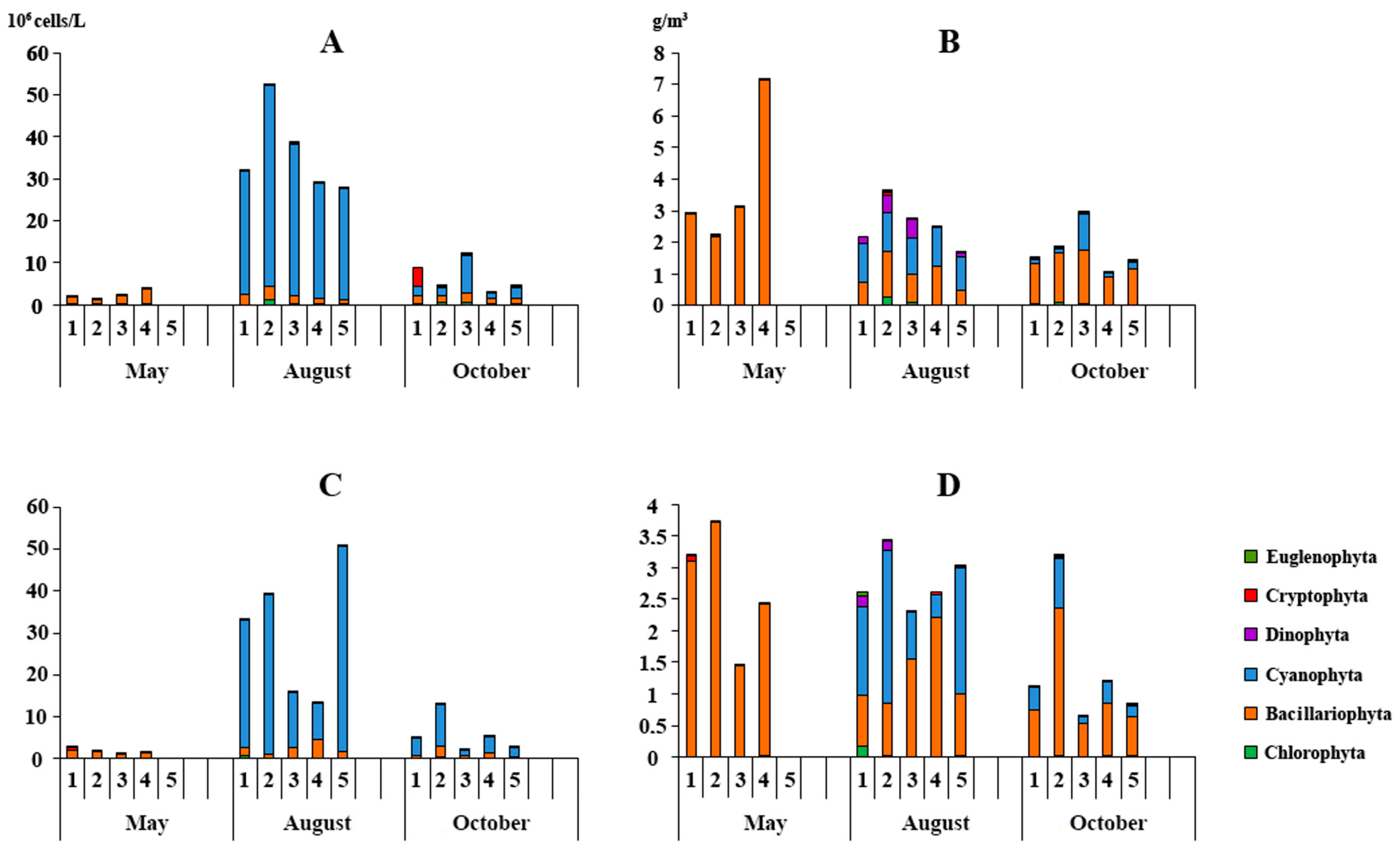
3.3.1. Phytoplankton

The taxonomic diversity of phytoplankton found in the upstream and downstream parts of the HPP amounted to 250 species taxa of algae and cyanobacteria, which belonged to eight divisions: Chlorophyta (36% of the total composition), Cyanobacteria (24%), Bacillariophyta (22%), Ochrophyta (8%), Dinophyta (5%), and others (1–3%). In the upstream, the abundance of phytoplankton during the growing season varied from 1.02 to 73.26 × 10⁶ cells/L, biomass—0.86–8.76 g/m³; in the downstream—from 1.08 to 52.31 × 10⁶ cells/L and 0.64–3.72 g/m³, respectively (

Table 1. Phytoplankton abundance (N, 10⁶ cells/L) and biomass (B, g/m³) on stations in the upstream and the downstream (surface horizon).

Stations	25 May 2022		8 August 2022		12 October 2022
	N	B	N	B	N	B
U1	1.66	2.91	31.71	2.19	8.76	1.48
U2	1.02	2.20	52.31	3.61	4.2	1.84
U3	1.99	3.12	38.45	2.77	11.91	2.93
U4	3.73	7.15	29.02	2.48	2.88	1.04
U5	–	–	27.67	1.68	4.18	1.39
D1	2.56	3.21	33.22	2.62	5.04	1.12
D2	1.75	3.73	39.25	3.42	13.04	3.18
D3	1.14	1.44	15.71	2.31	1.99	0.64
D4	1.35	2.43	13.26	2.61	5.32	1.19
D5	1.14	1.64	50.56	3.03	2.69	0.83

). The trophic state, determined by the phytoplankton biomass, was evaluated as mesotrophic–eutrophic in the upstream and as mesotrophic in the downstream.

We noted that the range of changes in quantitative indicators in integral and surface water samples, as well as the average values for the stream, remained similar both by season and in general over the study period (

Table 2. Average values of phytoplankton abundance (N, 106 cells/L) and biomass (B, g/m³) in the upstream and the downstream parts of the hydroelectric power plant during the study period. Designations: N surface *, B surface—abundance and biomass data for surface water horizon samples; N integral, B integral—the same parameters for integrated water samples.

Date	Upstream		Downstream
	N Surface * (N Integral)	B Surface (B Integral)	N Surface * (N Integral)	B Surface (B Integral)
25 May 2022 (spring)	2.10 ± 0.58 (1.85 ± 0.33)	3.85 ± 1.12 (3.81 ± 1.26)	1.70 ± 0.31 (1.29 ± 0.10)	2.70 ± 0.50 (2.41 ± 0.40)
8 August 2022 (summer)	35.83 ± 4.52 (45.05 ± 9.14)	2.55 ± 0.32 (2.87 ± 0.19)	30.43 ± 7.10 (21.95 ± 7.91)	2.80 ± 0.19 (1.78 ± 0.32)
12 October 2022 (autumn)	6.39 ± 1.70 (4.28 ± 0.95)	1.74 ± 0.32 (1.59 ± 0.24)	5.62 ± 1.96 (4.72 ± 0.72)	1.39 ± 0.46 (1.71 ± 0.21)
Seasonal average	15.68 ± 4.49 (17.06 ± 6.01)	2.63 ± 0.34 (2.76 ± 0.47)	13.36 ± 4.31 (9.32 ± 3.44)	2.27 ± 0.28 (1.97 ± 0.19)

). This may indicate a uniform distribution of phototrophic plankton in the photic zone as a result of active water mixing under the influence of currents as well as the operation of the hydroelectric power plant.

The composition of the dominant phytoplankton species varied at different periods of sampling. In May, during the period which was characterized by lower temperature and mineralization values and significant water consumption, diatoms appeared to be the dominant species of phytoplankton. Their contribution to the abundance and biomass was up to 98–99% of the values (Figure 13). The biomass of diatoms had a negative correlation with temperature (R = −0.78), calcium content (R = −0.71), bicarbonates (R = −0.77), and a positive one with water consumption (R = 0.68). On the contrary, with water heating, increasing content of ions and bicarbonates, and a decrease in water consumption observed in August, cyanobacteria predominated. In August, their share in the abundance was 90–95%, although their contribution to the biomass was less, amounting to 20–50% of the total values. A positive correlation was noted between the abundance and biomass of cyanobacteria with temperature (R = 0.93), conductivity (R = 0.83), and the content of calcium ions (R = 0.79), bicarbonates (R = 0.68), and nitrites (R = 0.72) and a negative one with water consumption (R = −0.62). It is known that planktonic cyanobacteria prefer low-flowing, well-heated eutrophic water bodies, and regulation of river flow can provoke their active development [43,44]. It was shown [44] that in the reservoirs of the Volga cascade, the appearance of a significant presence of cyanobacteria in plankton was noted at flow rates not exceeding 0.1 m/s, and their predominance in plankton was found at rates not exceeding 0.04 m/s. In August, we recorded the cyanobacteria predominance in abundance at all stations of upstream and downstream areas, where the variation in flow velocities could noticeably exceed the values mentioned above (up to 0.6 m/s). Despite the favorable temperature values, a sufficient amount of nutrients, and a high proportion of cyanobacteria in the overall indicators of phytoplankton development, the absolute values of abundance and biomass of these microorganisms turned out to be insignificant, corresponding to a low degree of water bloom in the reservoir. Apparently, it was the increased flow velocities and noticeable water circulation that prevented the potentially possible development of cyanobacteria in the zone of hydroelectric power station influence under the conditions of flow regulation. Despite the high buoyancy of cyanobacteria due to the presence of gas vacuoles in their cells, the proportion of these microorganisms in the surface-layer biomass was only slightly higher (1.2–1.3 times) than in the integrated water samples. This once again confirms the noticeable water mixing and the absence of stratification. In the upstream, dinoflagellates were noted among the biomass dominants, while in the downstream, their development was not noticeable. Flagellar algae, as well as cyanobacteria, are sensitive to turbulence [45], which could limit their development under conditions of more active water mixing. In October, an increase in the diatoms’ role was noted again, while the role of cyanobacteria decreased.

In the spatial distribution of the phytoplankton abundance and biomass in the downstream area on the days of sampling, differences were also noted. These differences were most noticeable (up to 2–6 times) during the period of insignificant water discharges in August and October (Table 1). On all sampling days, the lowest abundance and biomass values were recorded in surface-layer samples at station D3, where a shift in the flow direction and pronounced water circulation were noted, which made it difficult for algae cells to concentrate in the surface layers. More noticeable developmental indicators were noted at station D1, where increased concentrations of nutrients (

Table 3. Spatial and temporal distribution of hydrochemical parameters of water in the upstream (mean values with standard deviation).

Concentration. mg/L	Station U1 (in Front of the Entrance Channel)			Station U3 (500 m to the Left)			Station U4 (3 km to the Left)
	25 May 2022	8 August 2022	12 October 2022	25 May 2022	8 August 2022	12 October 2022	25 May 2022	8 August 2022	12 October 2022
Iron	0.05 ± 0.01	0.09 ± 0.02	0.16 ± 0.04	0.07 ± 0.02	0.08 ± 0.02	0.15 ± 0.04	0.06 ± 0.01	0.07 ± 0.02	0.08 ± 0.02
Magnesium	<0.05	<0.05	7.5 ± 1.2	<0.05	<0.05	6.8 ± 1.0	<0.05	<0.05	6.1 ± 0.9
Phosphorus	21.5 ± 3.2	0.19 ± 0.02	0.08 ± 0.02	21.5 ± 3.2	0.36 ± 0.04	0.09 ± 0.03	19.0 ± 2.9	0.28 ± 0.03	0.07 ± 0.02
Calcium	0.02 ± 0.01	21.9 ± 3.3	20 ± 3	0.02 ± 0.01	22.9 ± 3.4	17 ± 3	0.03 ± 0.01	23.1 ± 3.5	20 ± 3
Chlorides	5.1 ± 0.5	4.4 ± 1.1	5.0 ± 1.0	3.5 ± 0.8	4.6 ± 1.1	4.5 ± 1.1	3.8 ± 0.9	4.7 ± 1.1	5.3 ± 0.5
Nitrites	0.10 ± 0.01	0.4 ± 0.1	<0.2	0.02 ± 0.01	0.13 ± 0.04	<0.2	0.10 ± 0.01	0.18 ± 0.05	<0.2
Sulphates	106.0 ± 10.6	127.9 ± 12	17.7 ± 1.2	97.3 ± 9.7	125.7 ± 12	14.6 ± 1.5	106.4 ± 10.6	135.1 ± 13	16.2 ± 1.6
Nitrates	2.8 ± 0.6	0.32 ± 0.09	2.7 ± 0.5	0.9 ± 0.2	1.0 ± 0.2	2.3 ± 0.5	3.1 ± 0.6	0.33 ± 0.09	2.2 ± 0.4
Phosphates	0.05 ± 0.001	0.57 ± 0.11	0.23 ± 0.01	0.10 ± 0.01	1.1 ± 0.2	0.26 ± 0.05	0.10 ± 0.01	0.86 ± 0.17	0.21 ± 0.01
Ammonium ion	0.73 ± 0.11	0.14 ± 0.03	0.28 ± 0.11	0.75 ± 0.11	0.15 ± 0.03	0.29 ± 0.1	0.68 ± 0.10	0.13 ± 0.03	0.30 ± 0.12
Hydrocarbonates	85.4 ± 14.5	109.8 ± 13	104 ± 18	73.2 ± 12.5	103.7 ± 12	107 ± 18	79.3 ± 13.5	115.9 ± 14	110 ± 18
pH. pH units	6.5 ± 0.2	8.2 ± 0.2	7.1 ± 0.2	6.8 ± 0.2	8.14 ± 0.2	7.1 ± 0.2	7.3 ± 0.2	7.9 ± 0.2	7.2 ± 0.2
Total mineralisation	162 ± 31	156 ± 30	110 ± 20	130 ± 25	148 ± 28	115 ± 22	144 ± 27	146 ± 28	115 ± 22

) coming from the water flow were noted. In August, the maximum number of algae cells was noted at station D5, which was the furthest from the dam. The basis of the abundance at that time was created by cyanobacteria. Apparently, the transport with the channel flow, as well as wind surges, contributed to the concentration of cyanobacteria, the cells of which are characterized by buoyancy, in the surface layers of this part of the water area. However, due to the insignificant volumes of cyanobacterial cells, this group of phytoplankton did not make a significant contribution to the total biomass, the value of which turned out to be comparable with those of other stations at that time.

3.3.2. Zooplankton

To analyze the species structure of zooplankton cenosis and calculate ecological indices, it is necessary to accurately identify the species composition of aquatic organisms in the studied water bodies. In the composition of zooplankton in the waters of the pools, 35 species were found, among which rotifers (Rotifera) predominated—19 species. Cladocera and copepods (Copepoda) were represented by 11 and 5 species, respectively. Most of the species were cosmopolitans. An analysis of the ecological confinement of zooplankton species showed that obligate–planktonic species (51%) were more common among ecological groups; phytophilic (31%) and phytophilic–planktonic species (12%) were rare. The demersal species had the smallest share (3%) (Figure 14).

The species compositions of zooplankton in the upstream and downstream areas of the HPP were similar. Both areas were dominated by naupliar and copepodite stages of copepods. In May and August, the dominants and subdominants, along with them, included the cladocerans Bosmina longirostris, Daphnia cucullata, and Daphnia longispina. Rotifers Brachionus calyciflorus and Synchaeta pectinata appeared in the summer.

Indicators of the quantitative development of zooplankton in the upstream and downstream areas differed significantly by season (Figure 15A). The total abundance of zooplankton in the upstream area was higher in May and August; in the downstream area—in October. The maximum values of zooplankton biomass were recorded in August both above and below the HPP (Figure 15B).

The share of dead individuals of planktonic organisms in the total abundance and biomass of zooplankton throughout the study period was higher in the downstream area of the reservoir (Figure 15C,D). At the same time, in August, due to a significant increase in the number of dead individuals in the upstream area (at p ≤ 0.05), these indicators were at the same level.

The natural mortality of rotifers, cladocerans, and copepods as a percentage of the total abundance in the upstream and downstream areas was minimal in May and maximal in August (Figure 15C). Conversely, natural mortality as a percentage of total biomass peaked in May and declined by October (Figure 15D).

The mortality of zooplankton in the Gorky Reservoir can be associated with a number of factors. A fundamental one, in our opinion, is the change in water discharge, the maximum values of which were noted in May. At the known discharge, the proportion of mortality in the total number of zooplankton in the downstream reaches 15%, which is the norm and is confirmed by early studies of this type [36].

In August, the death of large limnic filter feeders of the genera Daphnia (D. cucullata, D. galeata) and Diaphanosoma (D. brachyurum, D. orghidani), predominantly developing here in summer, may be due to the influence of wind, causing convective mixing of water layers and organisms along with them [36]. In the downstream, however, the high numbers of dead individuals of large limnic filter feeders and predators are due to a greater extent to hydromechanical effects [36].

Another important factor affecting the mortality of populations is temperature, which has not a direct, but rather an indirect effect. Thus, an analysis of the literature data showed that the time of the peak and the magnitude of the natural mortality of zooplankton are controlled by the water temperature in the previous winter, early spring, and early summer [36].

3.4. Hydrochemistry

Table 3 and

Table 4. Spatial and temporal distribution of hydrochemical indicators of downstream water (mean values with standard deviation).

Concentration. mg/L	Station D1 (below the Entrance Channel)			Station D3 (500 m to the Left)			Station D4 (1 km to the Left)
	25 May 2022	8 August 2022	12 October 2022	25 May 2022	8 August 2022	12 October 2022	25 May 2022	8 August 2022	12 October 2022
Iron	0.07 ± 0.02	0.10 ± 0.02	0.098 ± 0.02	0.10 ± 0.02	0.09 ± 0.02	0.13 ± 0.03	0.10 ± 0.02	0.09 ± 0.02	0.22 ± 0.05
Magnesium	<0.05	<0.05	5.3 ± 0.8	<0.05	<0.05	7.4 ± 1.1	<0.05	<0.05	10.5 ± 1.6
Phosphorus	18.9 ± 2.8	0.23 ± 0.02	0.07 ± 0.02	18.1 ± 2.7	0.27 ± 0.03	0.09 ± 0.03	18.3 ± 2.8	0.21 ± 0.02	0.08 ± 0.02
Calcium	0.5 ± 0.2	21.6 ± 3.2	16.5 ± 2.5	0.02 ± 0.01	21.8 ± 3.3	21 ± 3	<0.02	22.8 ± 3.4	41 ± 5
Chlorides	2.6 ± 0.6	5.7 ± 1.4	5.7 ± 0.6	3.6 ± 0.9	4.4 ± 1.1	4.9 ± 1.2	4.1 ± 1.0	4.5 ± 1.1	5.2 ± 0.5
Nitrites	0.4 ± 0.1	0.41 ± 0.12	<0.2	0.06 ± 0.01	0.39 ± 0.11	<0.2	0.08 ± 0.01	0.41 ± 0.12	˂ 0.2
Sulphates	172.2 ± 17.2	121 ± 12	16.0 ± 1.6	83.0 ± 8.3	117 ± 12	14.9 ± 1.5	109.3 ± 10.9	132 ± 13	17.3 ± 1.7
Nitrates	6.9 ± 0.7	1.1 ± 0.2	1.8 ± 0.4	0.9 ± 0.1	1.8 ± 0.4	2.7 ± 0.5	2.7 ± 0.6	0.53 ± 0.11	1.8 ± 0.4
Phosphates	1.5 ± 0.2	0.72 ± 0.14	0.21 ± 0.01	0.10 ± 0.01	0.84 ± 0.17	0.26 ± 0.05	0.01 ± 0.001	0.63 ± 0.13	0.20 ± 0.01
Ammonium ion	0.61 ± 0.09	0.16 ± 0.03	0.30 ± 0.12	0.66 ± 0.09	0.16 ± 0.03	0.31 ± 0.12	0.74 ± 0.11	0.13 ± 0.03	0.32 ± 0.13
Hydrocarbonates	75.6 ± 12.9	109.8 ± 13	107 ± 18	72.0 ± 12.2	97.6 ± 11.7	104 ± 18	73.2 ± 12.5	115.9 ± 13	107 ± 18
pH. pH units	7.2 ± 0.2	7.8 ± 0.2	7.2 ± 0.2	7.1 ± 0.2	7.1 ± 0.2	7.2 ± 0.2	6.9 ± 0.2	7.2 ± 0.2	7.2 ± 0.2
Total mineralization	148 ± 28	150 ± 28	112 ± 23	130 ± 25	158 ± 30	114 ± 24	126 ± 24	144 ± 28	128 ± 24

present the results of analyses of water samples collected for hydrochemical parameter determination during the season (25 May 2022, 8 August 2022, and 12 October 2022) at three stations upstream of the HPP and three mirrored stations downstream of the HPP. It can be seen that most of the studied parameters have no significant spatial heterogeneity except for water salinity and nutrients in May and August sampling. Elevated values of mineralization at station U1 may be related to the inflow of water masses from right-bank tributaries (Yug and Trotsa). A comparison of the data on phytoplankton abundance and biomass with the content of nitrates and phosphates in water indicates their direct dependence. The highest values of both biogenic elements (phosphates and nitrates) and phytoplankton abundance and biomass on 25 May were typical for station U4 and on 8 August and 12 October for station U3. Such heterogeneity may be related to the difference in the current system (see Figure 5). In May, the highest water discharge was observed and in the vicinity of stations U1-U3, the flow was directed towards the discharge holes, while U4 was located at the side of the flow bringing water from the right bank. In other cases, flow vectors are directed toward station U3. There is also significant heterogeneity of nutrients in the downstream reach, with the highest values gravitating towards station D1, especially in May, which is associated with the discharge of bottom water.

3.5. Bottom Sediments, Benthos, and Specific Methane Flux

At stations away from the dam, despite the flow of the reservoir, the difference between bottom and surface water temperatures is greater, even during cool weather in late May (

Table 5. Results of measurements of hydro-ecological characteristics (nd—no data).

Station	Depth. m	Tsurf-Tbot. °C	Hygroscopic Humidity. %	OM. %	Diffusion Flux CH4 from BS mgC/m2 day	CH4. mkl/l (Surface/Bottom)	Specific Flux CH4. mgC/m2 day	CBW. mgO/m2 day	Aerobic Destruction. mgC/m2 day	Total Destruction. mgC/m2 day	Turbidity. NTU (Surface/Bottom)	pH (Surface/Bottom)
25–26 May 2022
U3	8	0.5	2.8	6.7	nd	2.6/1.6	nd	25	nd	nd	14/7	8.4/8.2
U2	8	0.1	1.3	4.0	0.03	1.5/1.3	nd	32	58	140	6/10	8.1/8.0
U11	11	1.4	7.9	23.3	0.20	3.7/2.7	2.5–8.0	84	177	181	6/nd	8.1/nd
U9	16	1.1	7.1	17.4	1.89	1.5/2.0	0.25	108	135	193	6/12	8.1/8.1
U13	9	1	5.5	11.8	0.14	3.1/3.1	1.9	98	213	272	5/5	8.1/8.1
24–25 August 2022
U1	20	0.9	0.7	1.9	nd	0.5/1.4	0.5	nd	nd	nd	nd/4.8	8.5/8.3
U3	8.5	2.0	1.6	8.6	1.89	0.4/0.5	1.8	235	262	418	nd/5.5	8.4/8.1
U5	14.5	2.2	3.1	7.1	3.34	0.5/4.3	468	176	88	913	nd/10.7	8.2/7.8
U6	9.5	2.8	8.5	13.9	0.35	0.6/3.3	0.1	309	221	974	nd/5.4	8.3/8.0
U12	18.5	3.2	6.8	17.1	2.45	0.4/61.9	1.7	349	334	366	nd/6	8.7/8.1
U11	9	2.9	nd	nd	nd	0.9/15.9	974	315	254	312	nd/6.3	8.9/8.4
U7	9.5	2.9	5.0	10.3	0.06	0.9/0.7	nd	362	317	515	nd/4.6	8.9/8.1
U14	18	3.1	7.1	16.2	0.95	0.2/0.2	1.9	424	352	229	nd 6/24	8.6/8.1
U8	17.5	3.1	6.6	14.9	8.13	0.2/1.1	3.1	235	262	418	11.4/30.9	9.0/7.8

). In August, at a distance from the dam, this difference over the channel stations increases from 0.9 at U1 to 3.1–3.2 °C at U12 and U14. This is due to the breakdown of stratification during the activation of runoff currents in the channel trough during releases, as discussed in the relevant section. At stations close to the dam at distances up to 2 km (U1–U3), the organic matter (OM) content in the bottom sediments (BS) does not exceed 10%. At distances of 4–5 km (U5–U7), its content increases to 10–14% and only at distances of 6–7 km (U8, U9, U12, U14) does it increase to 14–17%.

The hygroscopic moisture, as well as the organic matter content, were unevenly distributed in the dam area. Hygroscopic moisture is determined by particle size, on which the total surface area of particles per unit volume of soil and the size of pores between particles depend. Accordingly, the lowest values (0.7–1.6%) were observed at stations U1 and U3, where the BS were represented by silty sand and dense grey silt with thin (1–3 mm) fresh silt. Small values of hygroscopic moisture content were also observed at stations U2 and U5 (3.1–4.0), where dense brown and grey silt were sampled, respectively. Only at U5 was fresh silt observed, and this was found immediately above the dense silt with no transitional semi-liquid layer. The highest hygroscopic humidity is characteristic of BS at stations U6 and U11 (7.9–8.5%), which are located above the floodplain away from the channel trough. The bottom sediments there are represented by light brown silt with black interlayers and olive silt with plant remains. This suggests that in areas away from the mainstream, more organic-rich fine-dispersed silts are formed above the channel. At the surveyed channel stations U8 and U14 furthest from the dam, the bottom sediments are represented by two-layer light brown and grey silt with fresh silt of 1 mm, with black veins in the lower part of the column. The silt is of a sweeping consistency and differs from the sediments in the channel bed at the dam. Such differentiation of bottom sediments testifies to the influence of HPP discharges on the formation of the bottom complex, first of all, and also on the washing away of fine fractions due to mechanical impact during the activation of currents during discharges.

The characteristics caused by the interaction of the bottom water layer with BS also change in a regular way: oxygen consumption by bottom water (CBW) has the lowest values near the dam and increases at a distance from it by 3–4 times in May (from 25–32 to 135–213 mgC/m²day) and by 1.5–2 times in August (from 189–235 to 362–424 mgC/m²day). At channel stations, total degradation is slightly lower than at floodplain stations (229–418 and 312–515 mgC/m²day, respectively), which may be related to better aeration of bottom horizons at depths of up to 10 m. The specific methane flux from the water surface above the channel and floodplain stations is of the same order: 0.25–1.9 and 0.1–1.9, respectively. The small values are due to good aeration of the water column. However, two stations with exceptions were found: in the area of the left-bank floodplain (U11) and on the right bank (U5). The impressive values of methane flux may be due to the circulation peculiarities forming BS. Thus, at station U11, there is olive silt with small remains of vegetation, wood, and Dreissena polymorpha. At U5, the silt is grey, with black inclusions, but with a 1 cm layer of red silt. Compared to the neighboring stations, where the fresh silt layer is considerably thinner, it can be assumed that organic matter sinking to the bottom during water blooms is redistributed and accumulated away from the flow towards the dam.

At the neighboring station U6, there is no similar layer of fresh silt and the specific methane flux values are significantly lower. Station U5 is far enough away from the dam that the silt is not completely washed away at this site, but it is still under the dynamic influence of the dam: this station has maximum methane fluxes from the BS and from the surface, indicating the role of sediment agitation. Methane yield from bottom sediments could not be determined by the tube method at all stations due to difficulties in BS sampling. The patterns obtained indicate a lower flux from floodplain stations (0.06–1.81 mgC/m²day) than from channel stations (0.95–8.13 mgC/m²day), with the highest flux at station U8, which is farther away from the dam.

The results of benthic sampling revealed that the dam compartment within the study area is poor in benthic organisms. No benthos was found in the sediments at stations U3 and U9; chironomid biomass at U2, U11, and U13 was 1.7, 4.4, and 0.9 g/m² respectively, and mollusc biomass was 1.2–6.8 g/m², which differs from the data given for the whole of the dam’s reach in [46]. At the same time, the flooded channel areas were characterized by the presence of predominantly Dreissena polymorpha, whereas gastropod mollusks were found on the flooded floodplain.

In the downstream reach, the hydro-ecological characteristics at the stations were not fundamentally different, the bottom sediments were sand, and along the channel trough, it was sand with gravel. At station D1, the highest benthic (Dreissena polymorpha) biomass of 1000 g/m² was observed. Conditions in this area are very favorable for mollusks, providing hard substrate, good aeration, and flow. At station D5, the total biomass decreased to 206.5 g/m² and, in addition to Dreissena, Trichoptera was encountered.

4. Conclusions

This paper presents the results of the study of spatial and temporal variability of a wide range of hydrological parameters in the upstream section of the Gorky Reservoir based on the results of three expeditions in 2022 in connection with the task of assessing the impact of HPPs on the water environment. The paper presents data of measurements of hydrophysical, hydrooptical, hydrobiological, and hydrochemical water parameters, as well as benthos parameters, finds preliminary relationships between these parameters, and establishes the boundaries of HPP manifestation in the water area of the Gorki Reservoir. The results obtained from an idea of variable dynamics of water masses in connection with changes in water discharge through hydroelectric power plants, quickly manifested in a significant change in the structure of surface currents and, as a result, in the transfer of impurities (including areas of intensive blooming).

Active mixing of waters under the influence of currents, as well as the operation of the hydroelectric complex, contributed to the uniform distribution of phytoplankton in the water column of the photic zone of the reservoir. The horizontal distribution of phytoplankton was formed by local flow processes. The seasonal change in the main dominant groups (cyanobacteria, diatoms) was determined both by hydrological conditions and environmental parameters correlated with them (temperature, mineralization, nutrients).

The natural mortality of zooplankton, not related to predation, varied seasonally in accordance with quantitative development indicators. In percentage terms, the proportion of dead individuals was higher in the downstream of the HPP during the entire study period. A significant impact on mortality rates was exerted by the direct influence of hydroelectric power stations and a combination of hydrophysical parameters.

A complex system of currents, which is formed due to the periodicity of water discharges, leads to differences in the vertical distribution of characteristics in the water column with distance from the dam. Resuspension and sedimentation lead to the washout of secondary sediments in the vicinity of the dam, which affects the magnitude of the methane flux, exchange processes with the bottom, and the state of the benthos. The obtained results will be useful for the correct interpretation of satellite data, taking into account the spatial variability of the specific methane flux when calculating the total emission, and assessing potential sites of bottom sediment contamination as a result of sedimentation within dam areas.

References

1. Savichev, O.G.; Krasnoshchèv, S.Y.; Nalivaiko, N.G. River Flow Regulation; Tomsk Polytechnic University: Tomsk, Russia, 2009; p. 114. [Google Scholar]
2. Jorgensen, S.E.; Loffler, H.; Rast, W.; Straskraba, M. Lake and Reservoir Management, 1st ed.; Elsevier: Amsterdam, The Netherlands, 2005; p. 512. [Google Scholar]
3. Nilsson, C.; Reidy, C.A.; Dynesius, M.; Revenga, C. Fragmentation and Flow Regulation of the World’s Large River Systems. Science 2005, 308, 405–408. [Google Scholar] [CrossRef]
4. Palmer, M.; Ruhi, A. Linkages between flow regime, biota, and ecosystem processes: Implications for river restoration. Science 2019, 365, eaaw2087. [Google Scholar] [CrossRef]
5. Edelstein, K.K. Reservoirs of Russia: Ecological Problems, Ways of Their Solution; GEOS Publishers: Moscow, Russia, 1998; p. 277. [Google Scholar]
6. Goldenfum, J.A. Challenges and solutions for assessing the impact of freshwater reservoirs on natural GHG emissions. Ecohydrol. Hydrobiol. 2012, 12, 115–122. [Google Scholar] [CrossRef]
7. De Faria, F.A.; Jaramillo, P.; Sawakuchi, H.O.; Richey, J.E.; Barros, N. Estimating greenhouse gas emissions from future Amazonian hydroelectric reservoirs. Environ. Res. Lett. 2015, 10, 124019. [Google Scholar] [CrossRef]
8. Whiting, G.J.; Chanton, J.P. Greenhouse carbon balance of wetlands: Methane emission versus carbon sequestration. Tellus B 2001, 53, 521–528. [Google Scholar] [CrossRef]
9. Prairie, Y.T.; Alm, J.; Beaulieu, J.; Barros, N.; Battin, T.; Cole, J.; del Giorgio, P.; DelSontro, T.; Guérin, F.; Harby, A.; et al. Greenhouse gas emissions from freshwater reservoirs: What does the atmosphere see? Ecosystems 2018, 21, 1058–1071. [Google Scholar] [CrossRef]
10. Chen, Z.; Liu, Z.; Yin, L.; Zheng, W. Statistical analysis of regional air temperature characteristics before and after dam construction. Urban Clim. 2022, 41, 101085. [Google Scholar] [CrossRef]
11. Iakunin, M.; Abreu, E.F.; Canhoto, P.; Pereira, S.; Salgado, R. Impact of a large artificial lake on regional climate: A typical meteorological year Meso-NH simulation results. Int. J. Climatol. 2022, 42, 1231–1252. [Google Scholar] [CrossRef]
12. Karadžić, V.; Subakov-Simić, G.; Krizmanić, J.; Natić, D. Phytoplankton and eutrophication development in the water supply reservoirs Garaši and Bukulja (Serbia). Desalination 2010, 255, 91–96. [Google Scholar] [CrossRef]
13. Korneva, L.G. Phytoplankton of Volga River Basin Reservoirs; Kostroma Printing House: Kostroma, Russia, 2015; p. 284. [Google Scholar]
14. Mineeva, N.; Lazareva, V.; Livinov, A.; Stepanova, I.; Chuiko, G.; Papchenkov, V.; Korneva, L.; Shcherbina, G.; Pryanichnikova, E.; Perova, S.; et al. Chapter 2. The Volga River. In Rivers of Europe, 2nd ed.; Tockner, K., Zarfl, C., Robinson, C.T., Eds.; Elsevier: Amsterdam, The Netherlands, 2021; pp. 27–79. [Google Scholar]
15. Genkal, S.I.; Okhapkin, A.G.; Vodeneeva, E.L. Planktonic Centric Diatoms (Bacillariophyta, Coscinodiscaceae) of the Cheboksary Reservoir, Russia. Inland Water Biol. 2022, 15, 750–759. [Google Scholar] [CrossRef]
16. Molkov, A.; Fedorov, S.; Pelevin, V. Toward Atmospheric Correction Algorithms for Sentinel-3/OLCI Images of Productive Waters. Remote Sens. 2022, 14, 3663. [Google Scholar] [CrossRef]
17. Dobrokhotova, D.V.; Kapustin, I.A.; Molkov, A.A.; Leshchev, G.V. A study of the effect of hydropower operation regime on the redistribution of phytoplankton in the upper water layer in the dam section of the Gorki Reservoir. Sovrem. Probl. Distantsionnogo Zondirovaniya Zemli Iz Kosmosa 2023, 20, 242–252. [Google Scholar] [CrossRef]
18. Litvinov, A.C. About measurement of currents in reservoirs by EPV-2r recorders. Proc. Inst. Biol. Inland Waters USSR Acad. Sci. 1968, 16, 259–268. [Google Scholar]
19. Hydrometeorological Regime of Lakes and Reservoirs of the USSR. Reservoirs of the Upper Volga; Gidrometeoizdat: Leningrad, Russia, 1975; p. 292.
20. Kapustin, I.A.; Molkov, A.A. Structure of currents and depth in the lake part of the Gorky Reservoir. Russ. Meteorol. Hydrol. 2019, 7, 110–117. [Google Scholar]
21. Kapustin, I.A.; Ermakov, S.A.; Smirnova, M.V.; Vostryakova, D.V.; Molkov, A.A.; Cheban, E.Y.; Leshchev, G.V. On the formation of an isolated lens of a river runoff by a whirlpool in the Gorky reservoir. Sovrem. Probl. Distantsionnogo Zondirovaniya Zemli Iz Kosmosa 2021, 18, 214–221. [Google Scholar] [CrossRef]
22. Kapustin, I.A.; Vostryakova, D.V.; Molkov, A.A.; Danilicheva, O.A.; Leshchev, G.V.; Ermakov, S.A. Field observations of convergent currents in the near-surface layer of water using foam patterns in quasi-synchronous satellite optical images. Sovrem. Probl. Distantsionnogo Zondirovaniya Zemli Iz Kosmosa 2021, 18, 188–196. [Google Scholar] [CrossRef]
23. Schlezinger, D.R.; Taylor, C.D.; Howes, B.L. Assessment of zooplankton injury and mortality associated with underwater turbines for tidal energy production. Mar. Technol. Soc. J. 2013, 47, 142. [Google Scholar] [CrossRef]
24. Bickel, S.L.; Hammond, J.D.M.; Tang, K.W. Boat-generated turbulence as a potential source of mortality among copepods. J. Exp. Mar. Biol. Ecol. 2011, 401, 105. [Google Scholar] [CrossRef]
25. Dubovskaya, O.P. Natural Mortality of Zooplankton in the Reservoirs of the Yenisei Basin; Author’s Abstract of Ph.D. in Biological Sciences; The Zoological Institute RAS: St. Petersburg, Russia, 2006. [Google Scholar]
26. Zakonnov, V.V.; Zakonnova, A.V.; Tsvetkov, A.I.; Sherysheva, N.G. Hydrodynamic processes and their role in formation of bottom sediments in reservoirs of the Volga—Kama cascade. Trans. IBIW RAS 2018, 81, 35–46. [Google Scholar]
27. Labay, V.S. Benthos distribution in the lower rithral of the poronai river under the impact of some abiotic environmental factors. Trans. “SakhNIRO 2007, 9, 184–206. [Google Scholar]
28. Kemenes, A.; Melack, J.; Forsberg, B. Downstream emissions of CH4 and CO2 from hydroelectric reservoirs(Tucuruí, Samuel, and Curuá-Una) in the Amazon basin. Columbia Inland Waters 2016, 6, 1–8. [Google Scholar] [CrossRef]
29. Butorin, N.V.; Ziminova, N.A.; Kurdin, V.P. Bottom Sediments of Upper Volga Reservoirs; Nauka: Leningrad, Russia, 1975; p. 157. [Google Scholar]
30. RusHydro. Hydroelectric Power Station Reservoir Levels. Available online: https://rushydro.ru/informer/ (accessed on 14 July 2023).
31. Weather Archive in the Volga Hydro-Meteorological Observatory. Available online: https://rp5.ru/%D0%90%D1%80%D1%85%D0%B8%D0%B2_%D0%BF%D0%BE%D0%B3%D0%BE%D0%B4%D1%8B_%D0%B2_%D0%92%D0%BE%D0%BB%D0%B6%D1%81%D0%BA%D0%BE%D0%B9_%D0%93%D0%9C%D0%9E (accessed on 14 July 2023).
32. Vodeneeva, E.L.; Kulizin, P.V. Algae of the Mordovian Nature Reserve (Annotated List of Species); Flora and Fauna of Nature Reserves: Moscow, Russia, 2019; Volume 134, p. 62. [Google Scholar]
33. Guiry, M.D.; Guiry, G.M. AlgaeBase; World-Wide Electronic Publication; National University of Ireland: Galway, Ireland, 2021; Available online: http://www.algaebase.org (accessed on 14 July 2023).
34. Zhikharev, V.; Vodeneeva, E.; Kudrin, I.; Gavrilko, D.; Startseva, N.; Kulizin, P.; Erina, O.; Tereshina, M.; Okhapkin, A.; Shurganova, G. The Species Structure of Plankton Communities as a Response to Changes in the Trophic Gradient of the Mouth Areas of Large Tributaries to a Lowland Reservoir. Water 2023, 15, 74. [Google Scholar] [CrossRef]
35. Okhapkin, A.; Sharagina, E.; Kulizin, P.; Startseva, N.; Vodeneeva, E. Phytoplankton community structure in highly-mineralized small gypsum karst lake (Russia). Microorganisms 2022, 10, 386. [Google Scholar] [CrossRef] [PubMed]
36. Dubovskaya, O.P. Non-predatory mortality of the crustacean zooplankton, and its possible causes (a review). Biol. Bull. Rev. 2009, 70, 168–192. [Google Scholar]
37. Dzyuban, A.N. Experiment in evaluating methane emissions in water bodies of urbanized territories in the Rybinsk reservoir basin. Water Resour. 2010, 37, 583–585. [Google Scholar] [CrossRef]
38. Sweerts, J.; Bar-Gilissen, M.; Cornelse, A.; Cappenberg, T.E. Oxygen-consuming processes at the profundal and littoral sediment-water interface of a small meso-eutrophic lake. Limnol. Oceanogr. 1991, 36, 1124–1133. [Google Scholar] [CrossRef]
39. Elrod, V.A.; Berelson, W.M.; Coale, K.N.; Johnson, K.S. The flux of iron from continental schelf sediments: A missing sourse of global budgets. Geophys. Res. Lett. 2004, 31, L12307. [Google Scholar] [CrossRef]
40. Martynova, M.V. Bottom Sediments as a Component of Limnic Ecosystems; Nauka: Moscow, Russia, 2010; p. 243. [Google Scholar]
41. Bastviken, D.; Santoro, A.; Marotta, H. Methane emissions from Pantanal, South America, during the low water season: Toward more comprehensive sampling. Environ. Sci. Technol. 2010, 44, 5450–5455. [Google Scholar] [CrossRef]
42. Bastviken, D.; Cole, J.; Pace, M.; Tranvik, L. Methane emissions from lakes: Dependence of lake characteristics, two regional assessments, and a global estimate. Glob. Biochem. Cycles 2004, 18, GB4009. [Google Scholar] [CrossRef]
43. Mihaljević, M.; Stević, F. Cyanobacterial blooms in a temperate river-floodplain ecosystem: The importance of hydrological extremes. Aquat. Ecol. 2011, 45, 335–349. [Google Scholar] [CrossRef]
44. Rakhuba, A.V. Assessment of the Influence Exercised by the Hydrodynamic Regime on the Phytoplankton Development and the Water Quality of the Kuibyshev Reservoir. Uchenye Zap. Kazan. Univ. Seriya Estestv. Nauk. 2020, 162, 430–444. [Google Scholar] [CrossRef]
45. Miracle, M.R.; Vicente, E.; Pedrós-Alió, C. Biological studies of Spanish meromictic and stratified karstic lakes. Limnetica 1992, 8, 59–77. [Google Scholar] [CrossRef]
46. Frolova, E.A.; Bayanov, N.G.; Minin, A.E.; Minina, L.M. Macrozoobenthos of the Gorky reservoir. Taxonomic structure and quantitative development. Proc. Mordovian State Nat. Reserve 2020, 25, 381–392. [Google Scholar]
Figure 1. Location of the Gorky Reservoir and general view of its lake part (NASA “Blue Marble” image (https://visibleearth.nasa.gov/collection/1484/blue-marble, accessed on 20 July 2023).
Water 15 03070 g001
Figure 2. Scheme of the studied area in the upstream section of the Gorky Reservoir in 2022. Blue points correspond to stations in upstream (U) and downstream (D) areas. Red lines define transects AB and AC in the upstream area as well as EF in the downstream area, where vertical profiling was performed; start point of each transect (A, E) is marked by a rhombus; arrows define movement direction. Green arrows indicate the direction of the Volga River’s flow.
Water 15 03070 g002
Figure 3. Daily-averaged water discharge at the hydropower plant based on 2018–2022 data.
Water 15 03070 g003
Figure 4. Graphs of water discharge by month for the ice-free period of the 2022 year.
Water 15 03070 g004
Figure 5. The spatial distribution of water currents on the 0.6 m horizon in the upstream and downstream areas of the hydroelectric power plant on 25 May 2022 (A), 8 August 2022 (B), and 12 October 2022 (C).
Water 15 03070 g005
Figure 6. Vertical distributions of water current velocity characteristics (AC), temperature (Temp) (DF) chlorophyll a concentration (GI), fluorescence component of dissolved organic matter (fDOM) (J,K), dissolved oxygen (DO) (L,M), and conductivity (Cond) (N,O) in the upstream area of the hydroelectric power plant on 25 May 2022 (A,D,G,J,L,N), 8 August 2022 (B,E,H,K,M,O), and 12 October 2022 (C,F,I). Designations A and B correspond to start and end points of transect AB (see Figure 2).
Water 15 03070 g006aWater 15 03070 g006b
Figure 7. Vertical flow profiles 400 m below the hydroelectric power plant on 25 May 2022 (A), 8 August 2022 (B), and 12 October 2022 (C). The drawing in the bottom (D) row is similar to the one above it, but it is based on measurement data obtained after 2 h. Designations E and F correspond to start and end points of transect EF (see Figure 2).
Water 15 03070 g007
Figure 8. Vertical distribution of temperature (Temp) (AC) chlorophyll a concentration (DF), fluorescence component of dissolved organic matter (fDOM) (G,H), dissolved oxygen (DO) (I,J), and conductivity (Cond) (K,L) below the hydroelectric power plant on 25 May 2022 (A,D,G,J,K), 8 August 2022 (B,E,H,J,L), and 12 October 2022 (C,F). Designations E and F correspond to start and end points of transect EF (see Figure 2).
Water 15 03070 g008
Figure 9. Variations in current magnitude (A,C,E) and direction (B,D,F) at three depths of 1 m (A,B), 3 m (C,D), and 6 m (E,F) on windy (blue curves) and windless (red curves) days. Designations A and B correspond to start and end points of transect AB (see Figure 2).
Water 15 03070 g009
Figure 10. The standard deviation of current magnitude (A,C,E) and direction (B,D,F) at three depths of 1 m (A,B), 3 m (C,D), and 6 m (E,F) on windy (blue curves) and windless (red curves) days. Designations A and B correspond to start and end points of transect AB (see Figure 2).
Water 15 03070 g010
Figure 11. Averaged current for the 3–6 m layer plotted over all days of measurements.
Water 15 03070 g011
Figure 12. Variations in flow magnitude (A) and direction (B) at 6 m depth as a function of water discharge of the hydroelectric power plant. Designations A and B correspond to start and end points of transect AB (see Figure 2).
Water 15 03070 g012
Figure 13. Seasonal abundance (A,C) and biomass (B,D) dynamics of different phytoplankton groups in the nearby hydroelectric power plant (1st row—upstream; 2nd row—downstream). Numbers 1–5 indicate station numbers.
Water 15 03070 g013
Figure 14. The ratio of the presence of zooplankton species of the main ecological groups nearby the hydroelectric power plant.
Water 15 03070 g014
Figure 15. Seasonal dynamics of the abundance (A,C) and biomass (B,D) of zooplankton within 2022 (1 row—total abundance and biomass; 2 series—abundance and biomass of dead individuals; U—upstream, D—downstream).
Water 15 03070 g015