Abstract
Large-amplitude internal waves (IWs) with strong lateral shear forces can cause destructive effects on marine engineering structures. In this study, a large eddy simulation (LES) method was employed to simulate the generation and propagation of IWs in a three-dimensional numerical wave tank, and the pressure distribution, flow field characteristics, and force behaviors of two tandem cylinders under the coupling effect of the IWs and slope terrain were studied. The influence mechanism of the normalized value of center-to-center spacing (L) and the diameter of the cylinder (D), i.e., (L/D), on the strength of the vortex disturbance between cylinders was studied by comparing the simulation results of two tandem cylinders with those of a single cylinder (SC) to further explore the mechanical response characteristics of the upstream cylinder (P1) and downstream cylinder (P2). The simulation results showed that the vortex interaction between cylinders is the critical factor that affects the forces acting on the cylinders. The strength of the vortex disturbance could be distinguished by the dimensionless critical center-to-center spacing between cylinders (Lc/D = 3.0). When L/D ≤ Lc/D, the vortex disturbance was severe, causing P1 and P2 to experience significant horizontal positive forces and negative forces, respectively. In the case of L/D > Lc/D, the forces acting on both cylinders gradually returned to those on a single cylinder.
1. Introduction
Internal waves (IWs) are the density stratification phenomena caused by vertical density differences in fluid salinity or temperature in various waters, which then cause fluctuations in the density interface (pycnocline) [1]. IWs have the characteristics of large amplitude, long period, and tremendous energy [2]. The IWs generated in stratified strong shear environments pose a serious threat to the supporting structures of risers, drilling platforms, or cross-sea bridges in the complex hydrodynamic environments of the near shore or estuaries [3]. Therefore, IWs are an important consideration in the design of underwater supporting structures.
Many scholars have conducted research on the characteristics of IW forces acting on underwater structures. Cai et al. [4] adopted Morison’s empirical formula to study the characteristics of the forces and moments exerted by IWs on a cylinder in a shear flow environment. Yang Fan et al. [5] established a mathematical model simulating the interaction between IWs and underwater vehicles in a two-layer fluid system, and analyzed the changes in horizontal forces, vertical forces, and moment of the submarine under the action of IWs. Wang Lingling et al. [6,7] employed physical experiments and numerical simulations to compare the force characteristics of cylinders with different shapes in IW environments. Helfrich [8] conducted a series of physical investigations to explore the propagation characteristics of IWs over slope terrains, including the phenomena of climbing and shallow fragmentation. The experimental results indicated that the IWs generated significant vertical mixing, and approximately 10–20% of the wave energy was consumed during vertical mixing. During the propagation of IWs over the coastal slope, continuous changes in the waveform had a continuous impact on the hydrodynamic characteristics, leading to shear instability, turbulent mixing [9], and exacerbating the shear effect of the density thermocline [10]. When the slope terrain causes the thickness of the upper and lower layers to be equal, the polarity of the waveform may even flip [11], transitioning from a depression wave to an elevation wave [12], thereby causing flow and vortex direction reversal. Accordingly, the topography has a significant impact on the propagation and evolution of IWs, greatly altering the hydrodynamic characteristics.
Moreover, Zdravkovich [13] noted that when underwater cylinders are arranged at a certain center-to-center distance, the resultant forces on multiple cylinders, as well as the surrounding flow field, are significantly different from those of a single cylinder (SC) at the same Reynolds number. Gopalan [14] numerically studied the flow field characteristics around two tandem cylinders and found that the center-to-center spacing between the cylinders has a significant influence on the flow field. The forces on the cylinders undergo sudden changes at a critical spacing. When the spacing (L) is less than the critical spacing (Lc) [15], the vortex disturbance between the cylinders will greatly affect the flow field evolution, leading to unpredictable changes in the flow field, pressure distribution, and force behaviors [16]. Wang [17] numerically studied the influence of the spacing between two tandem cylinders on the intensity of the vortex disturbance, exploring the mechanical properties of P1 and P2.
In summary, IWs can easily cause instability and damage to underwater engineering supporting structures, even leading to loss of control events. IWs have become a catastrophic environmental factor that must be considered in the design process of engineering supporting structures in complex stratified water environments. However, there have been few investigations on the force characteristics of cylinders in the coupled environment of slope terrain and IWs, and it is rare to find related studies on the forces acting on multicylinder structures in such a complex environment. In this study, a series of numerical simulations were carried out to solve the above engineering problems by establishing a three-dimensional numerical wave tank and adopting LES technology to examine the influence mechanism of IWs on the mechanical response mechanism of two tandem cylinders over the slope topography. The research findings can provide a reference for safety and stability research on cylindrical supporting structures in stratified strong shear slope environments. In Section 1, the research background and significance are presented. Section 2 provides the governing equations used in the numerical simulation. In Section 3, the numerical model is established and validated. In Section 4, the mechanical laws and flow field characteristics of P1 and P2 are discussed, and the conclusions are given in Section 5.
2. Governing Equation
(1) Momentum equations and continuity equations
In the description of the incompressible viscous fluid three-dimensional transient motion process, the Navier–Stokes equations (NS) are adopted:
where ρ is the density of the fluid; (i = 1, 2, 3) are the three direction coordinates of the Cartesian coordinate system; and t is the time. Correspondingly, p is the pressure; u is the velocity term; f is the body force; and µ is the kinematic viscosity.
(2) Scalar transport equation
Scalar transport equations are used to describe the transport processes of water density of different layers in this study:
where C is the scalar volume concentration; k is the molecular diffusion coefficient; S is the source term or the sink term; and is the density of clean water.
(3) Turbulence model
The large eddy simulation (LES) is a spatial low-pass filtering technique employed to capture turbulent fluctuations. It separates large-scale vortexes from small-scale vortexes by a filter function. The large-scale vortexes are directly simulated, and relatively the small-scale vortexes are enclosed by models.
where the overbar represents the filtering function; the subgrid stress tensor ; the subgrid scale flux . As a function that includes the filtering scale and deformation rate tensor, the expression of turbulent eddy viscosity at time t can be described as:
where Cs is the Smagorinsky constant and Δ is the filtered scale. In the IW environment, Cs changes with time and space. In this paper, Germano’s dynamic procedure method is adopted to determine [18]. The deformation rate tensor can be expressed as:
3. Numerical Models
In this study, a three-dimensional numerical tank with slope terrain and two tandem cylinders is used to simulate the generation and evolution of depression IWs and the force mechanism of the cylinders (upstream cylinder P1 and downstream cylinder P2) over the slope using LES technology. The three-dimensional dimensions of the numerical model are length (X) × width (Z) × height (Y) = 4 m × 0.3 m × 0.3 m, respectively. The dimensions of the slope terrain are length (X) × width (Z) × height (Y) = 2.15 m × 0.3 m × 0.1 m, respectively. P1 is located at the width center of the slope platform. The coordinates of the bottom center point are located at: (x, y, z) = (2.0, 0.15, 0.15), and the diameter of the cylinder D = 5 cm. The dimensionless center-to-center spacing between P1 and P2 is defined as L/D. Figure 1 illustrates the sketch map of the three-dimensional numerical tank.
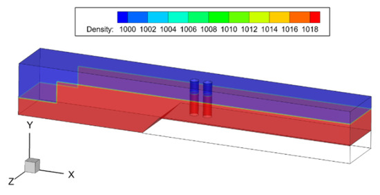
Figure 1.
Sketch map of three-dimensional numerical tank.
The formula for calculating the dimensionless horizontal resultant force acting on a cylinder in an IW environment can be defined as:
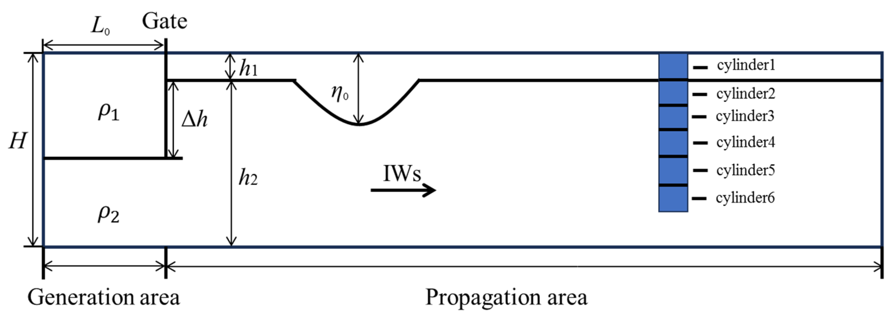
where is the horizontal resultant force on the cylinder in this numerical simulation; A is cylinder windward (frontal) side; g is the gravitational acceleration; and H is the total depth in the water tank. The stratified water parameters in the numerical tank are set as follows: the total water depth of the tank is H = 30 cm; the upper layer water density is 0.998 g/cm3, and the layer thickness ; the lower layer water density is 1.020 g/cm3, and the layer thickness . The depression IWs are produced by the gravity collapse method [19] in this simulation. The numerical tank is divided into two parts along the X direction: the wave generation area and the propagation area. The height difference between the generation area and the propagation area is the step height, and the length of the generation area is the step length. The slope angle in the model is = 45°. The specific parameters of the numerical tank are shown in Figure 2.
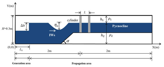
Figure 2.
Layout diagram of the specific parameters of the numerical tank.
3.1. Numerical Methods and Boundary Conditions
The large eddy simulation (LES) technique is used to simulate the generation and evolution of the IWs of a depression type in a three-dimensional numerical tank. The LES model of Smagorinsky type is a versatile turbulence model that can be applied to various flow studies, including wall-bounded turbulence as well as free shear flows like jets [20,21] and stratified flows of internal waves [22,23]. The finite-volume method is employed to discretize the control equations. The pressure implicit with splitting of operators (PISO) algorithm is employed to couple velocity and pressure, ensuring mass conservation and thus obtaining the pressure field. The diffusion and convection terms are discretized using the second-order central difference scheme and the second-order upwind scheme, respectively, and the time step is discretized by the second-order implicit scheme.
The left boundary of the wave generation region, the bottom, the tank sidewalls, and the surface of the cylinders are all set as nonslip solid-rigid wall boundaries. To avoid IWs from reflecting, the right end of the tank is defined as a Sommerfeld radiation boundary [24]. The tank top adopts the “rigid-lid” approximation to ignore the influence of surface waves [25].
3.2. Grid Independent Analysis
The corresponding Reynolds number of the internal waves environment [23] is calculated in this paper, where is the wave amplitude, is the wave phase speed, and is the kinematic viscosity. can be expressed as:
where co is the linear velocity of IWs.
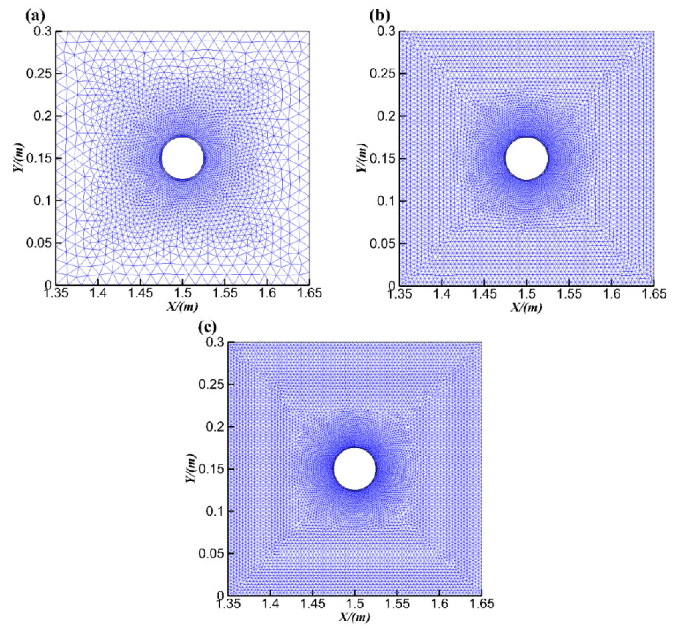
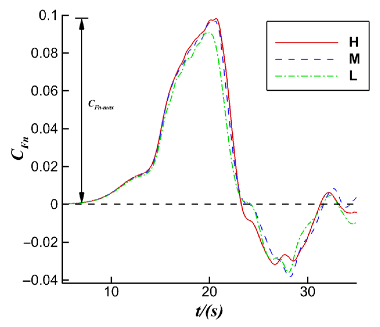
Grid independence analysis is conducted based on an SC in the environment without terrain, when ηo/H = 0.0575, as shown in Figure 3. Detail views of the grid around the cylinder with different grid densities are illustrated in Figure 4a–c. Figure 5 shows the calculation results of the IW horizontal resultant forces corresponding to the three grid density cases. When the grid density increases from a low density (L) to a moderate density (M), on the cylinder clearly changes, with a difference of 7.2% in between the two cases. The difference in between a moderate density (M) and a high density (H) is very slight, with only a difference of 0.5%. Considering that computing resources can be saved and the IWs’ propagation process and the force behaviors of the cylinder can be accurately simulated simultaneously, it is feasible to choose a moderate density grid to discretize the computational domain. The grid independence analysis details are shown in Table 1.
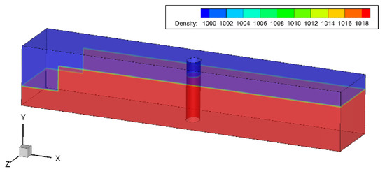
Figure 3.
Schematic diagram of the grid independent analysis model.
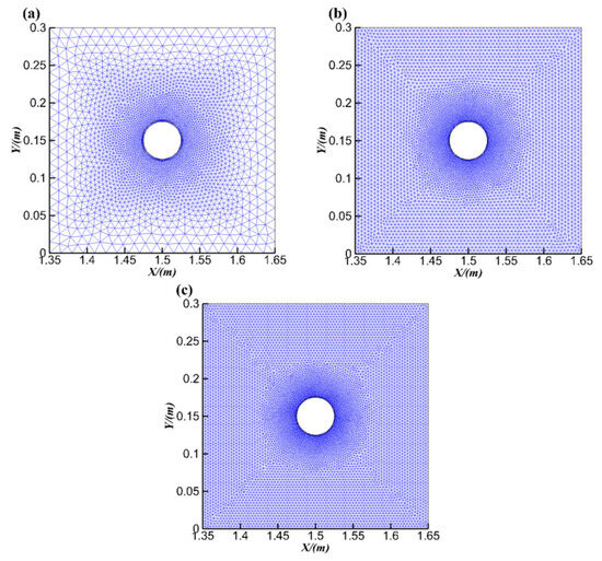
Figure 4.
Detail view of the grid around the cylinder periphery. (a) L (low density), (b) M (moderate density), (c) H (high density).
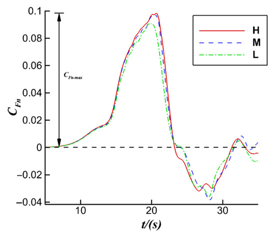
Figure 5.
Grid independence analysis results of the IW forces on the SC (ηo/H = 0.0575).

Table 1.
Details of the grid independence analysis.
3.3. Numerical Simulation Results Verified by the Physical Experimental Results
The physical model experiment conducted by Wang Fei [26] is used to validate the numerical model in this study. The dimensions of the tank are length (X) × width (Z) × height (Y) = 16.0 m × 0.35 m × 0.57 m, respectively. The upper layer of clear water has a thickness of h1 = 0.95 m and a density of = 1000 kg/m3, while the lower layer has a thickness of h2 = 0.475 m and a density of = 1024 kg/m3. By opening the gate, IWs are generated and they propagate towards the right end under the influence of gravity collapse [19,27], as shown in Figure 6. A vertical cylinder is placed at a distance of 10 m from the left end of the tank. The cylindrical body is divided into six segments, each with a length of 8 cm, and numbered from top to bottom as cylinders 1–6.
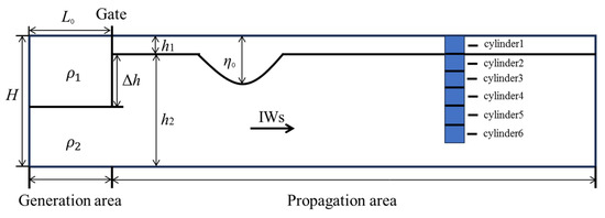
Figure 6.
Schematic diagram of the experimental setup by Wang Fei.
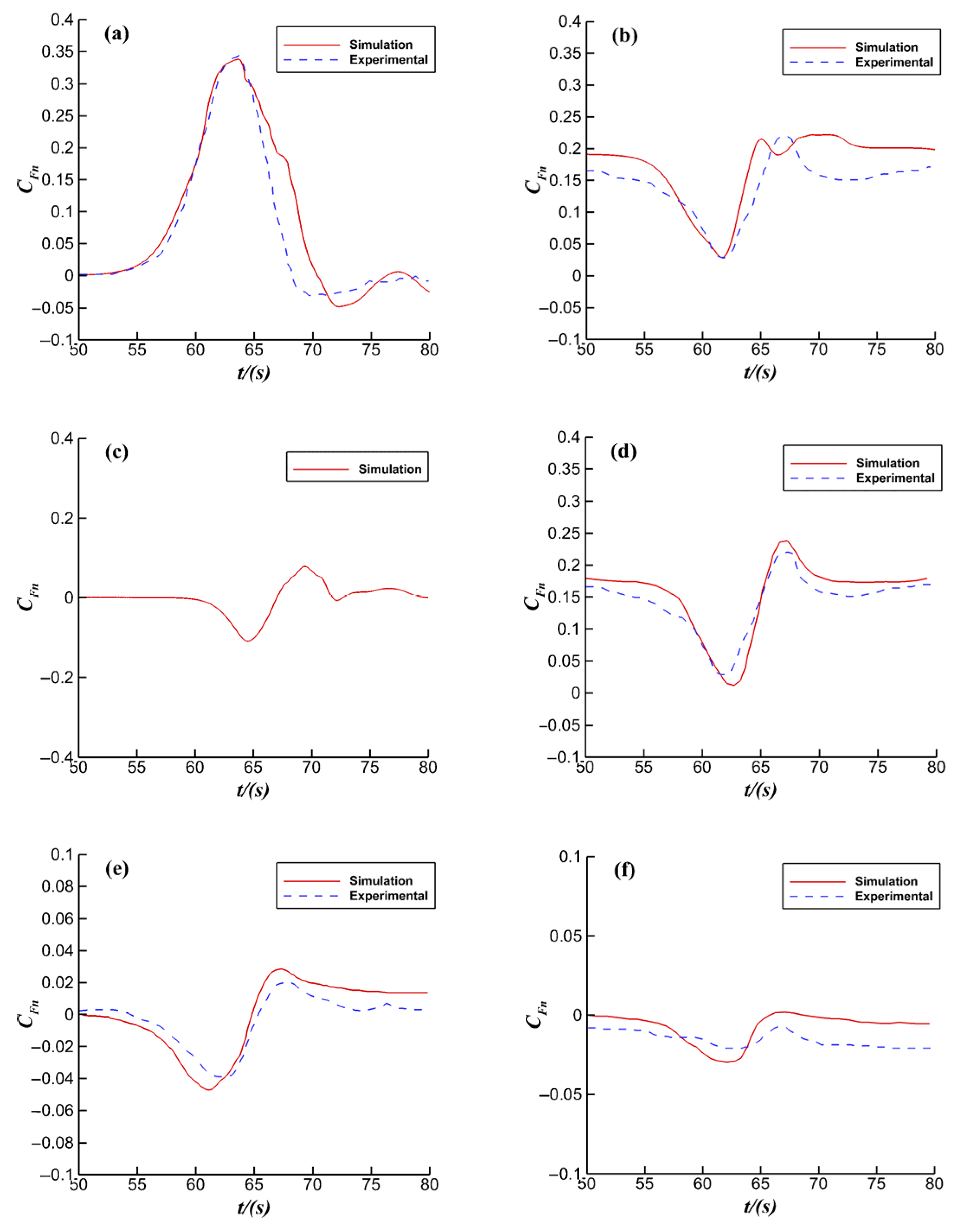
The dimensions and the water stratification parameters of the numerical tank are set according to the physical model experiment conducted by Wang Fei [26]. Following the modeling and meshing methods described earlier, a three-dimensional numerical model was established. The model verification results are shown in Figure 7, where the numerical calculations are in good agreement with the experimental measurements, except for the missing experimental data for case cylinder 3. This indicates that the established numerical tank in this study is reliable and capable of accurately simulating the propagation of IWs and the forces on the cylinders.
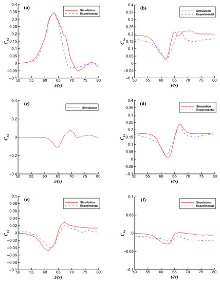
Figure 7.
Comparison of force duration curves between physical model experiments and numerical simulations. (a) Cylinder 1, (b) Cylinder 2, (c) Cylinder 3, (d) Cylinder 4, (e) Cylinder 5, (f) Cylinder 6.
4. Results and Analysis
4.1. Effects of Slope Terrain on the Forces Acting on SC and Two Tandem Cylinders
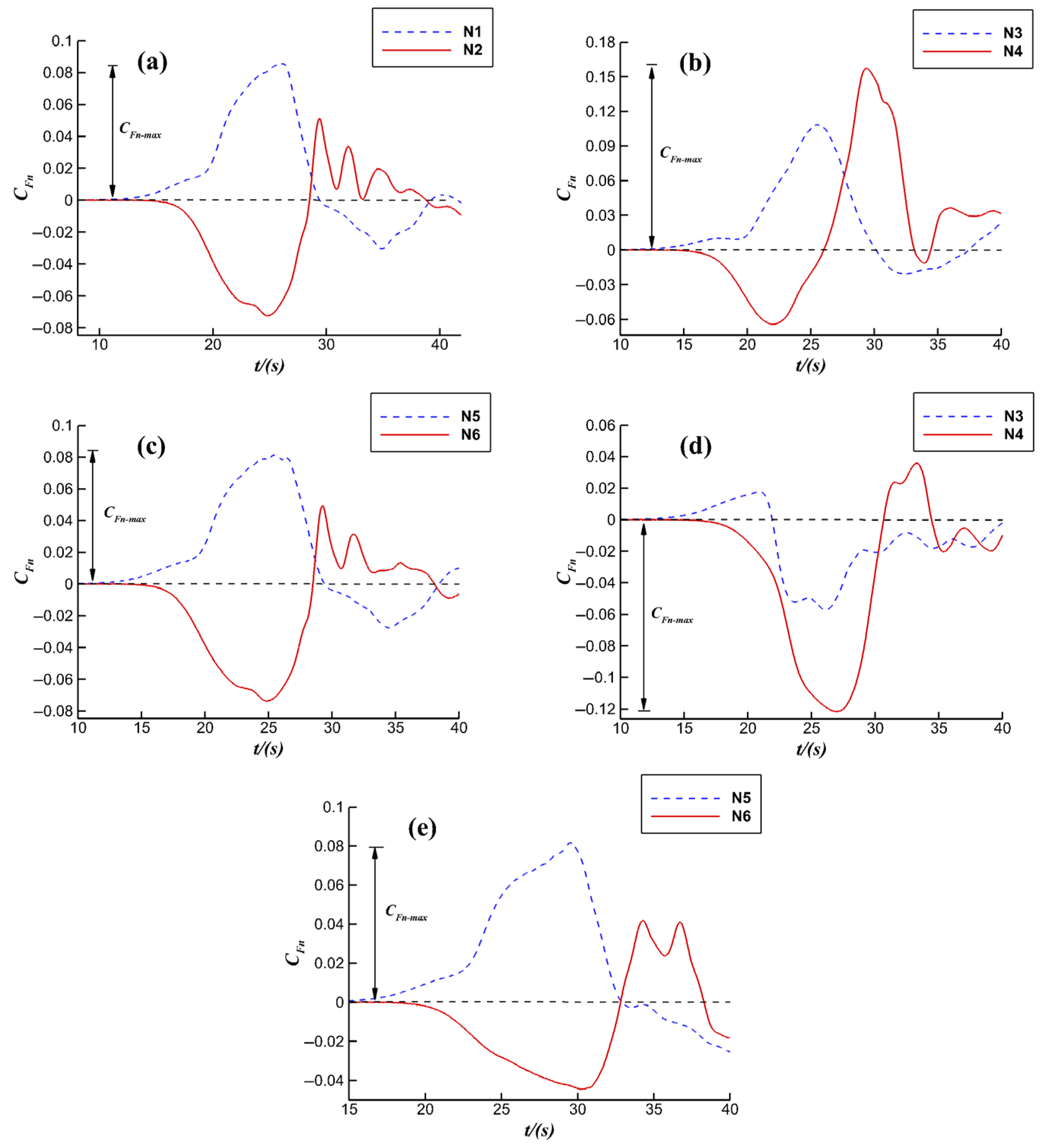
Figure 8a–e presents the duration curves of the dimensionless horizontal resultant forces acting on the single cylinder, upstream cylinder P1, and downstream cylinder P2 for different cases, including the no-slope SC model (Case N1), the slope terrain SC model (Case N2), the no-slope double cylinder model (Cases N3 and N5), and the slope terrain double cylinder model (Cases N4 and N6), with a dimensionless wave amplitude of ηo/H = 0.057. The case details are provided in Table 2.
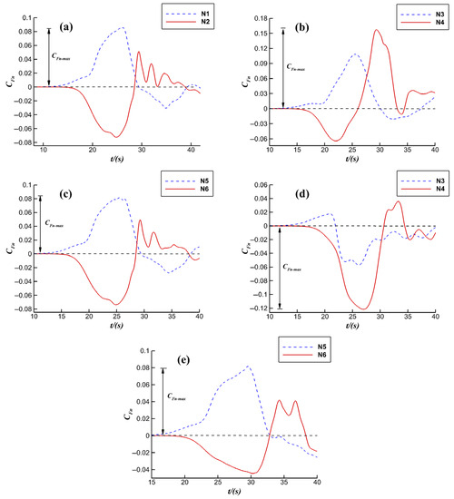
Figure 8.
Comparison of the duration curves of for different cases. (a) SC, (b) P1 (L/D = 1.5), (c) P1 (L/D = 6.0), (d) P2 (L/D = 1.5), (e) P2 (L/D = 6.0).
Table 2.
Detailed parameters in cases.
From Figure 8a,c,e, when the spacing between the two cylinders is large, the maximum values of the horizontal resultant forces on P1 and P2 in the slope terrain cases are negative and slightly smaller in magnitude than those in the no-slope case. When the spacing between the cylinders is small, as shown in Figure 8b,d, there is a strong interaction between P1 and P2, resulting in more complex forces on the cylinders. A detailed analysis will be provided in the following sections. To further analyze the force characteristics of the cylinders under different cases, the worst condition of the forces on the cylinders () in each case is selected as the research object.
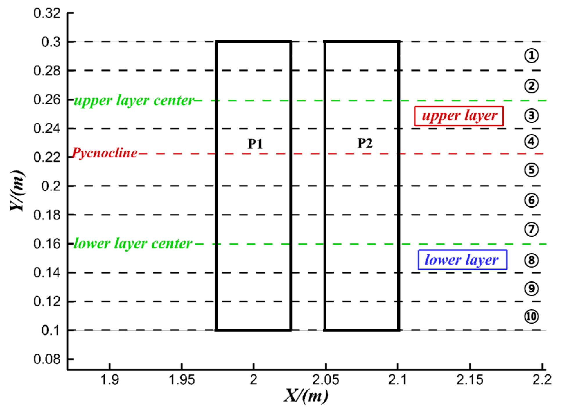
When depression-type IWs propagate, the flow in the upper and lower layers is in opposite directions. In the upper layer, the direction of the flow is the same as the IW propagation direction. In the lower layer, however, the flow direction is opposite to the IW propagation direction. Each cylinder body is divided into 10 segments along the vertical direction, with each segment having a length of 0.02 m, as shown in Figure 9. The portion of the cylinder located in the upper water layer is called the “upper parts”, while the portion in the lower water layer is referred to as the “lower parts”. In the following analysis, the vertical distribution of the dimensionless horizontal force coefficient () along the cylinder sections is calculated. The definition of is based on Equation (10), which is similar to that of .

Figure 9.
Schematic diagram of cylinder vertical segments.
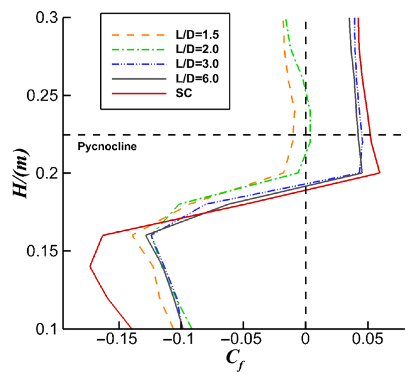
When the spacing between the cylinders is large, as observed from Figure 10a,c,e, the slope terrain leads to a decrease in the positive horizontal force on the cylinder (in the same direction to that during IW propagation) in the upper layer and an increase in the negative horizontal force on the cylinder (in the opposite direction to that during IW propagation) in the lower layer. This results in a negative on the cylinders in the presence of slope terrain. When the spacing between the cylinders is small, see Figure 10b,d, the vertical distribution of for the cylinders can be either positive or negative. However, the presence of slope terrain increases the magnitudes of for both P1 and P2 (as shown in Figure 8b,d).
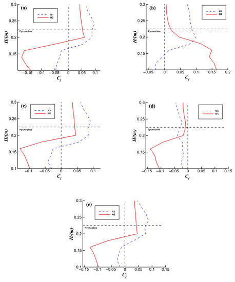
Figure 10.
Vertical distribution of comparison diagram for different cases (CFn = CFn−max). (a) SC, (b) P1 (L/D = 1.5), (c) P1 (L/D = 6.0), (d) P2 (L/D = 1.5), (e) P2 (L/D = 6.0).
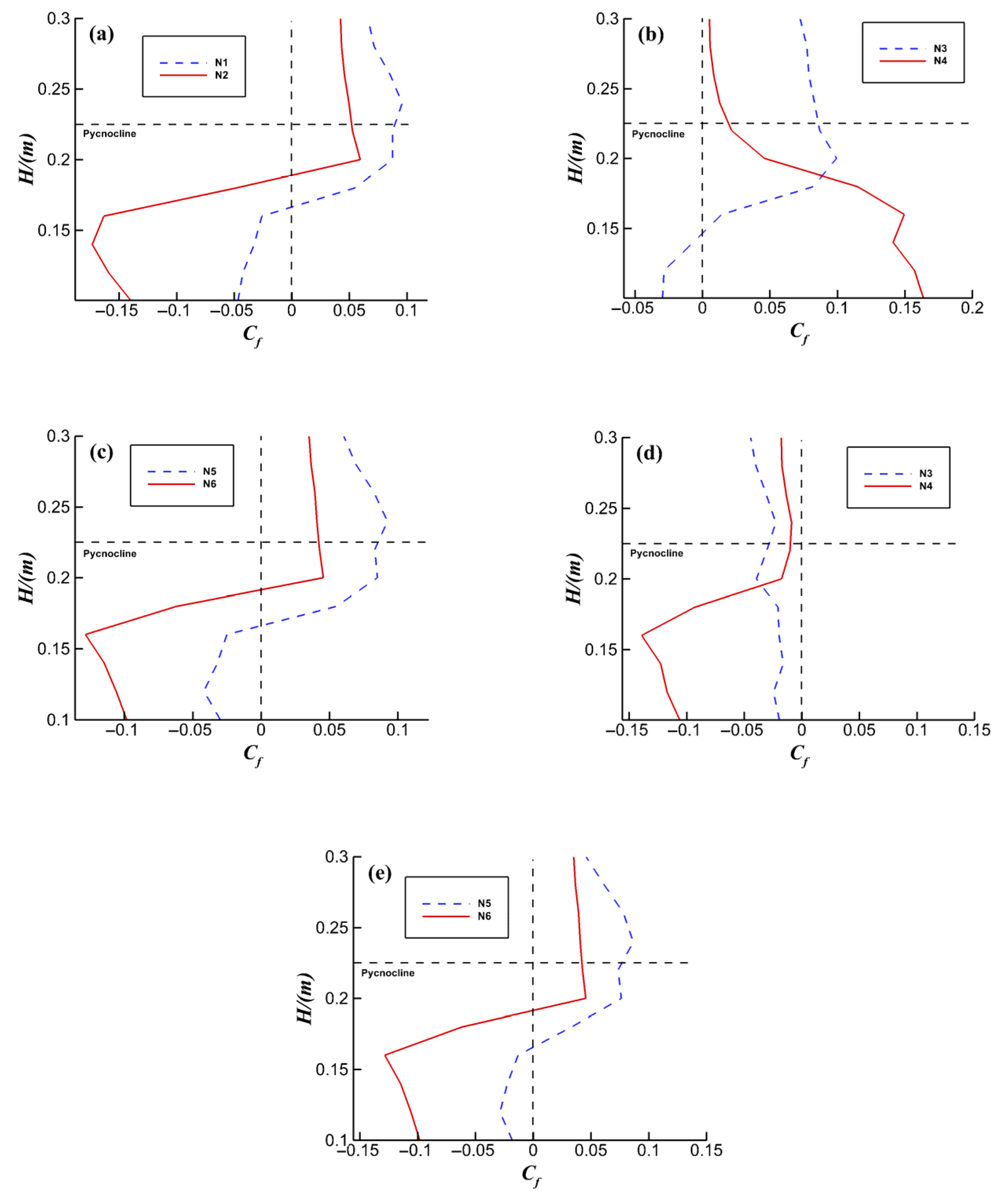
Further analysis of the differences in forces under different cases is conducted by comparing the pressure distribution along the circumference of the cylinder at two specific sections: Y = 0.16 m (the mid-depth of the lower layer) and Y = 0.26 m (the mid-depth of the upper layer). The schematic diagram of the cylinder circumferential angles is shown in Figure 11.

Figure 11.
Schematic diagram of circumferential angle definition.
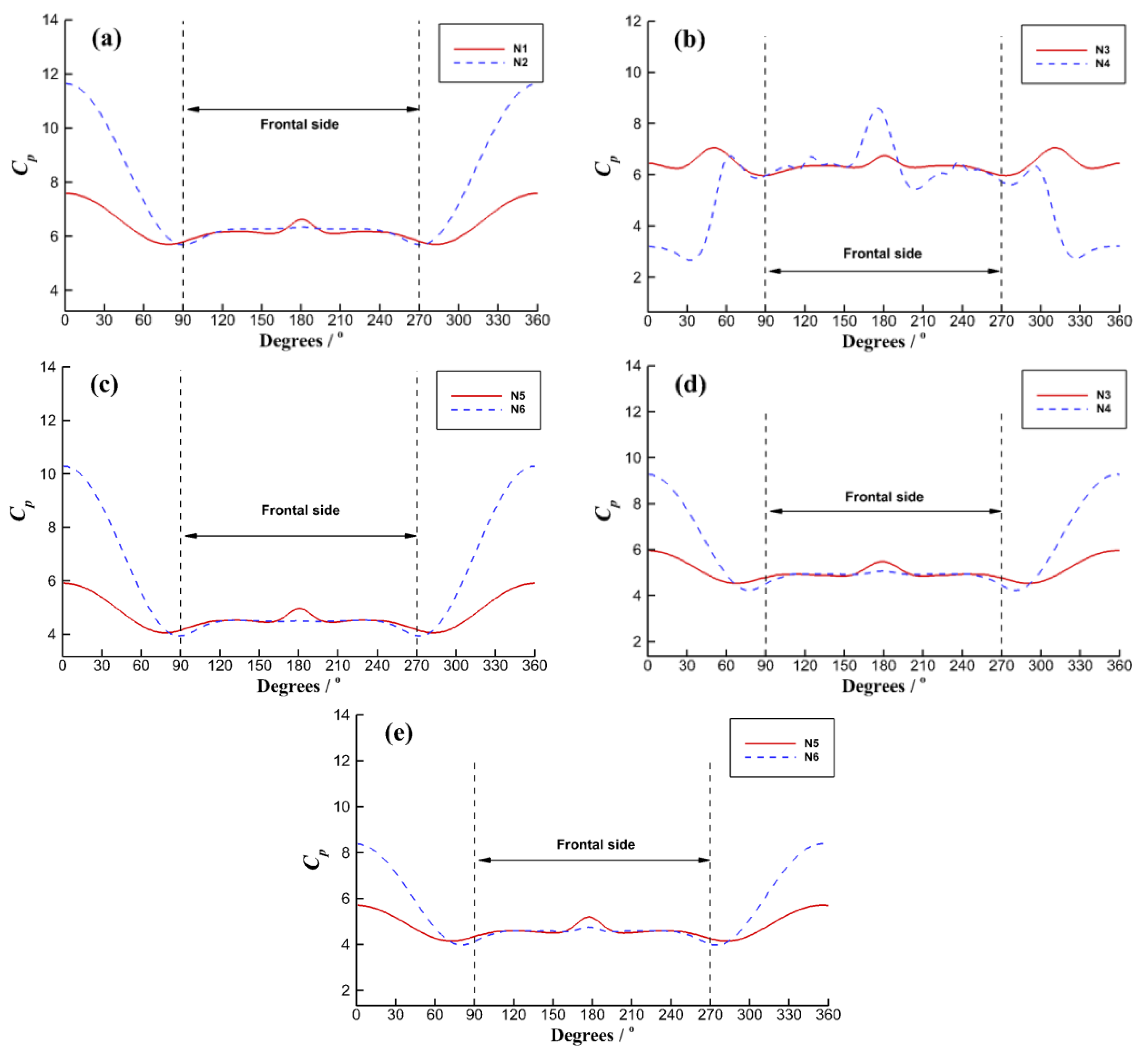
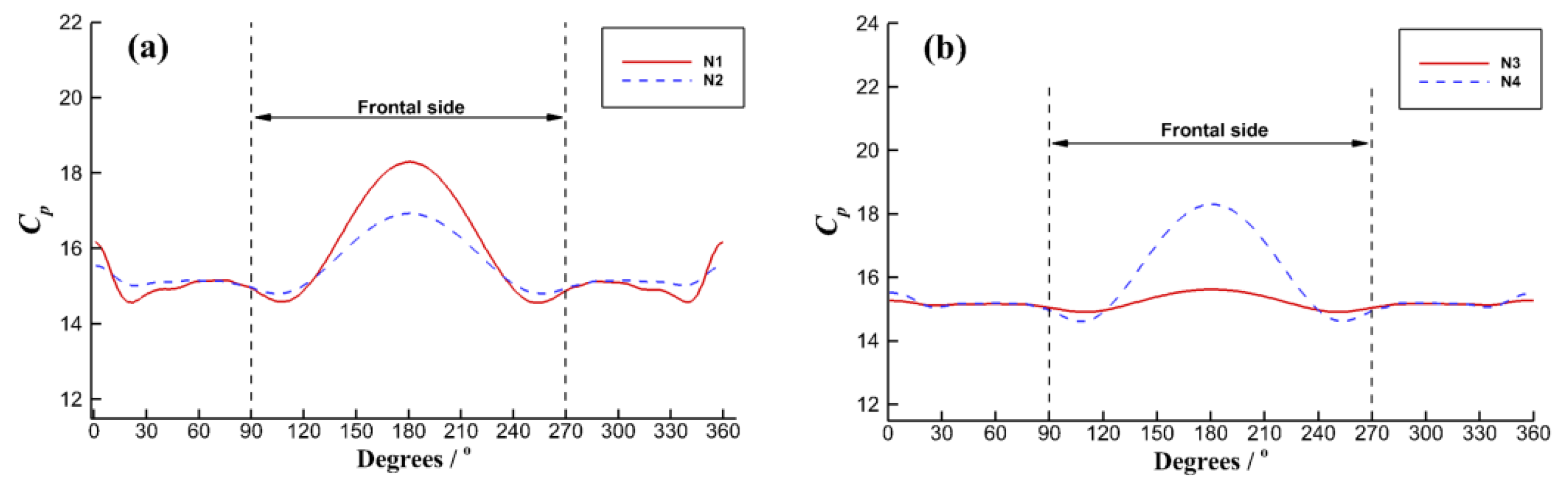
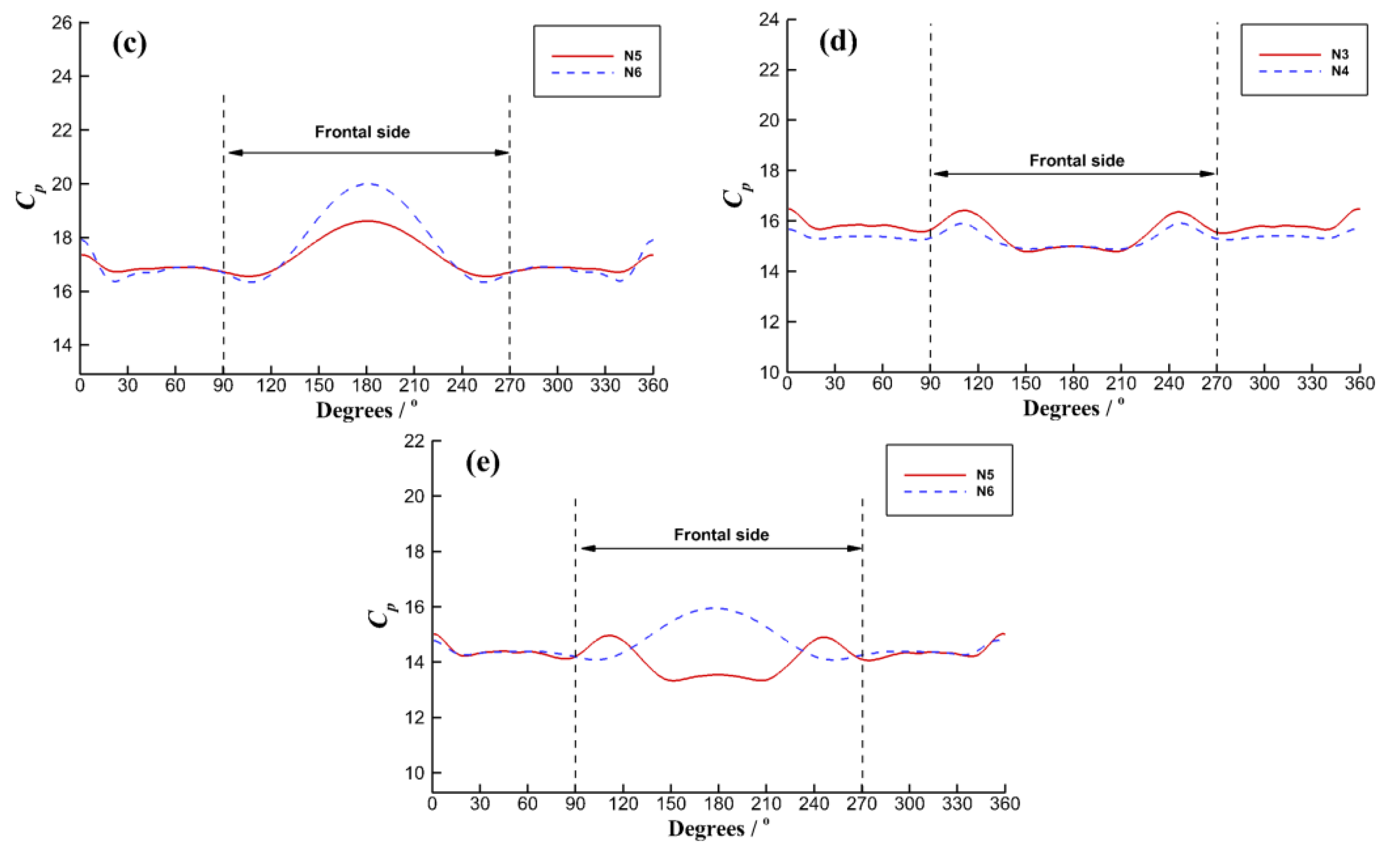
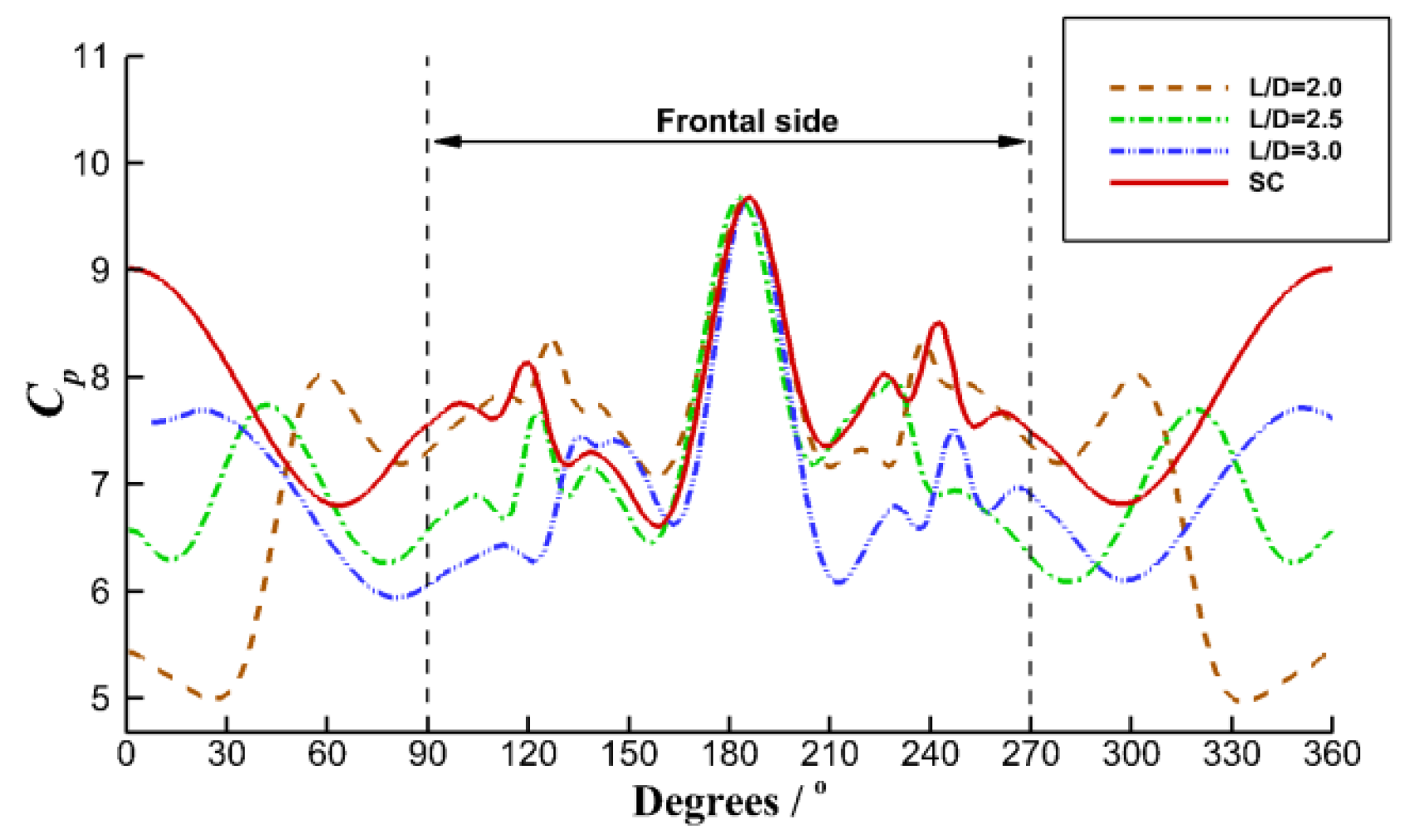
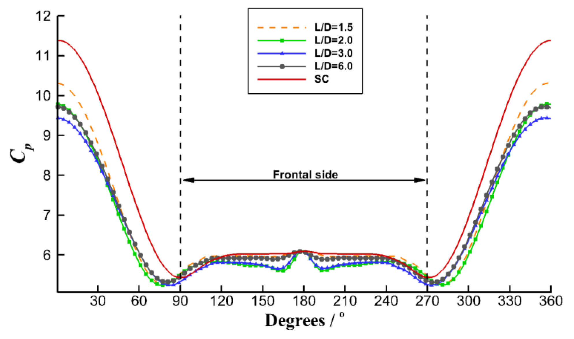
Figure 12a–e presents the circumferential pressure distribution for different cases at Y = 0.16 m, where Cp is the pressure on the periphery of the cylinder cross section. In the lower layer, the slope terrain has a significant impact on the pressure on the lee side of P1 and P2, while the pressure differences on the frontal side are minimal. In the upper layer, as shown in Figure 13, the presence of slope terrain leads to significant changes in the pressure distribution on the frontal side of P1 and P2, with minimal differences in the pressure distribution on the lee side. These results indicate that the slope terrain has a substantial influence on the pressure and forces experienced by single and two tandem cylinders. In the following sections, the mechanisms of the combined effects of slope topography and IWs on the flow field, pressure distribution, and forces acting on P1 and P2 will be specifically analyzed, considering different L/D cases.
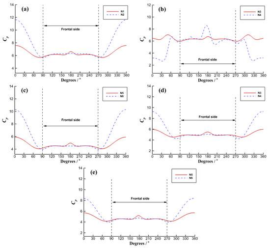
Figure 12.
Comparison of cylinder circumferential pressure distribution (Y = 0.16 m). (a) SC, (b) P1 (L/D = 1.5), (c) P1 (L/D = 6.0), (d) P2 (L/D = 1.5), (e) P2 (L/D = 6.0).
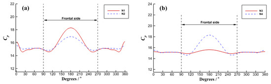
Figure 13.
Comparison of cylinder circumferential pressure distribution (Y = 0.26 m). (a) SC, (b) P1 (L/D = 1.5), (c) P1 (L/D = 6.0), (d) P2 (L/D = 1.5), (e) P2 (L/D = 6.0).
4.2. Effects of L/D on the Force Behaviors and Flow Field Characteristics for P1
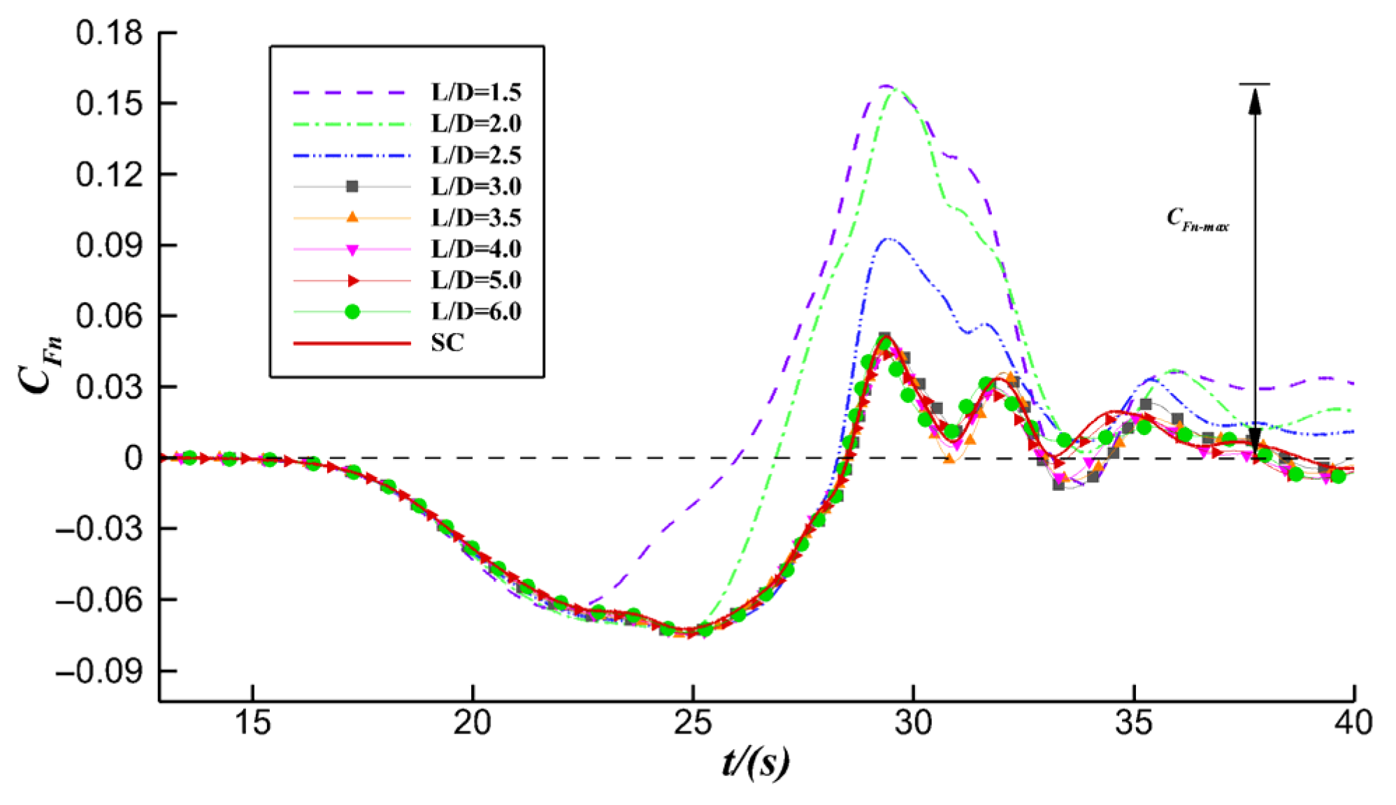
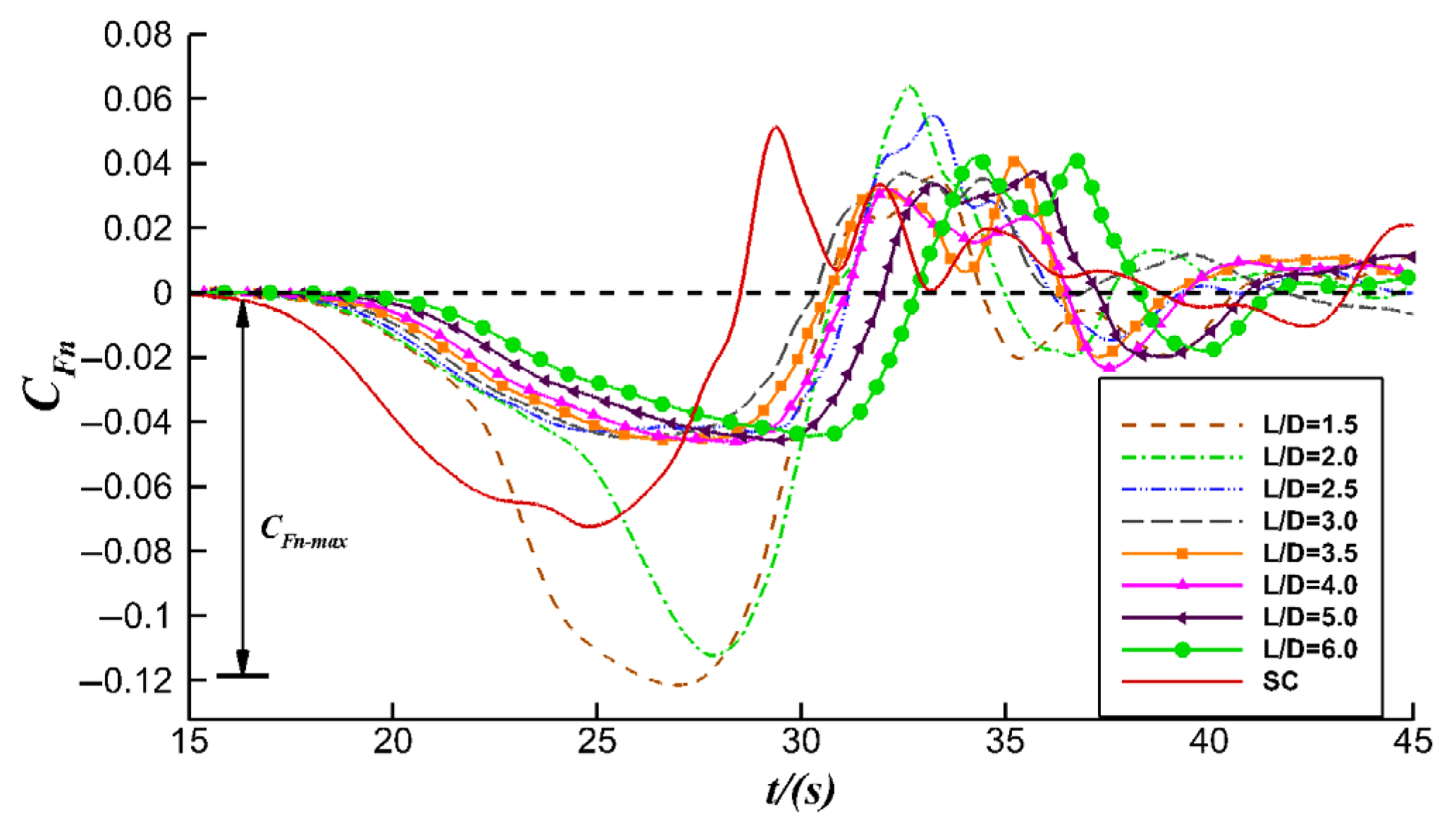
Figure 14 presents the duration curves of acting on P1 for eight different L/D cases (1.5 ≤ L/D ≤ 6, cases C2–C9) compared with an SC case (case C1), when ηo/H = 0.057. As shown in the figure, acting on the cylinder changes with time, and the overall trend of the force curves remains consistent across the nine cases. When L/D < 3.0, the maximum value for P1 is observed at L/D = 1.5. For 3.0 ≤ L/D ≤ 6, the force duration curves of P1 exhibit a high degree of similarity, with less variation in the value as L/D changes. These results indicate that L/D = 3.0 can be defined as the dimensionless critical spacing Lc/D. When L/D < Lc/D, there is strong mutual interference between the cylinders. Alternatively, when L/D ≥ Lc/D, the mutual interference gradually diminishes. Moreover, when the spacing between the cylinders is sufficiently large, the force acting on P1 approaches that on the SC.
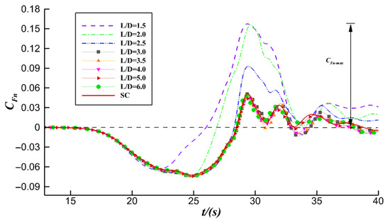
Figure 14.
Comparison of the duration curves of for different cases for P1.
Next, we will compare the pressure distribution and flow field of P1 and SC for different L/D ratios to reveal the mechanical mechanism of P1 in an IW environment. The specific cases are detailed in Table 3.
Table 3.
Simulation cases for studying the forces acting on P1.
4.2.1. Distinction of the Flow Field and Pressure Distribution between P1 and SC (L/D = 1.5)
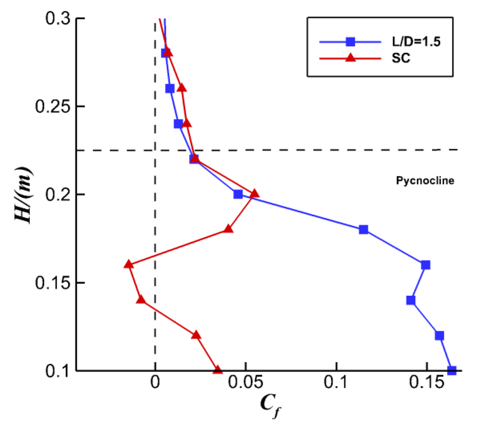
Figure 15 shows the vertical distribution of for P1 for the cases of SC and L/D = 1.5. P1 and the SC exhibit almost identical distributions in the upper layer. However, in the lower layer, P1 experiences significantly higher values compared to the SC, resulting in a larger postive on P1. Therefore, when L/D = 1.5, the focus is primarily on examining the force characteristics of the lower parts of the cylinder. The following analysis will further investigate the force mechanisms acting on P1 by comparing the flow field evolution and circumferential pressure distribution when Y = 0.16 m.
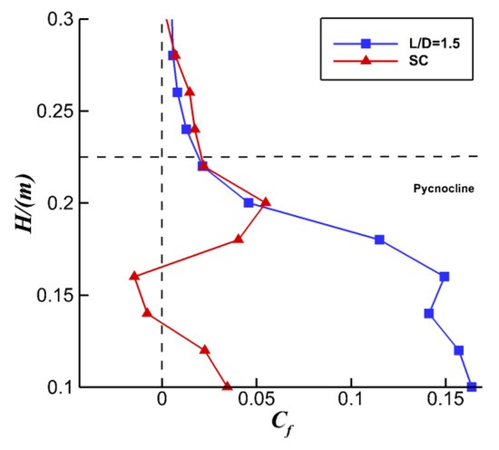
Figure 15.
Vertical distribution of comparison diagram of SC and P1 (CFn = CFn−max), L/D = 1.5.
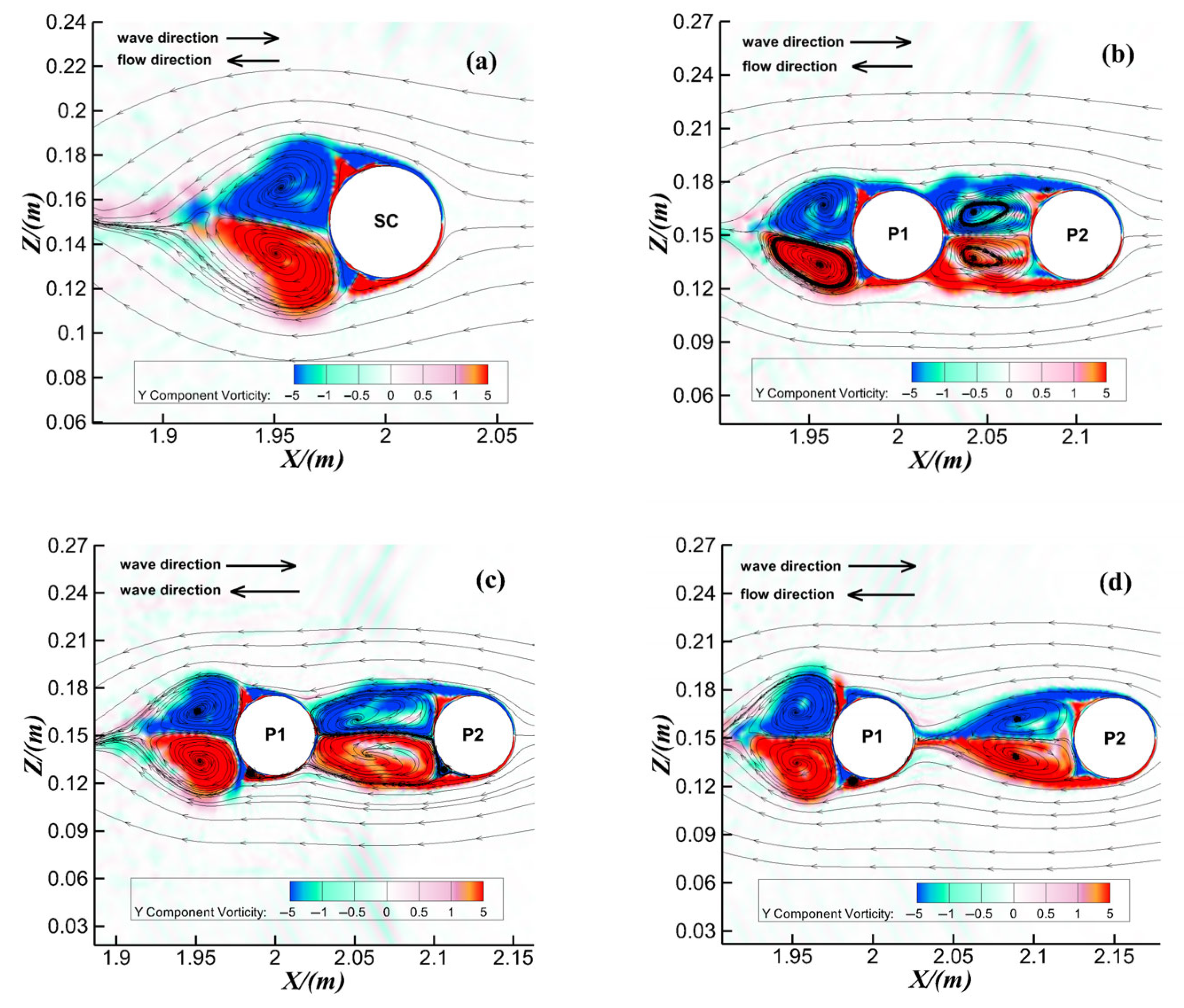
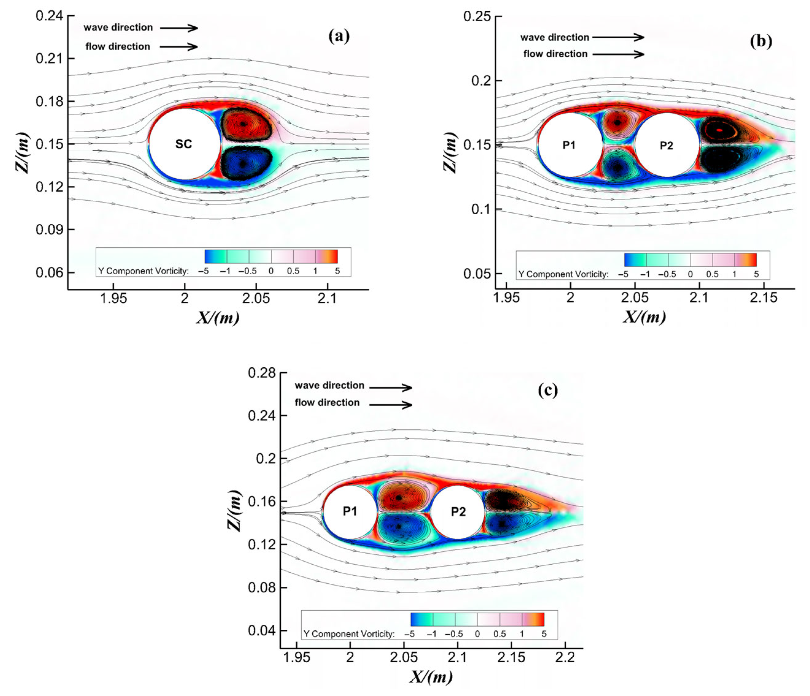
Based on the vorticity contour maps shown in Figure 16a,b, it can be observed that when L/D = 1.5, there is an intense disturbance between the two cylinders, and the development of vortices behind P1 is suppressed. The presence of vortices caused by P2 clearly contributes to altering the flow field distribution around P1 in the downstream vortex region.
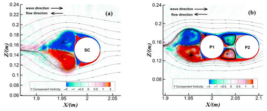
Figure 16.
Flow field characteristics comparison diagram (Y = 0.16 m). (a) SC, (b) L/D = 1.5.
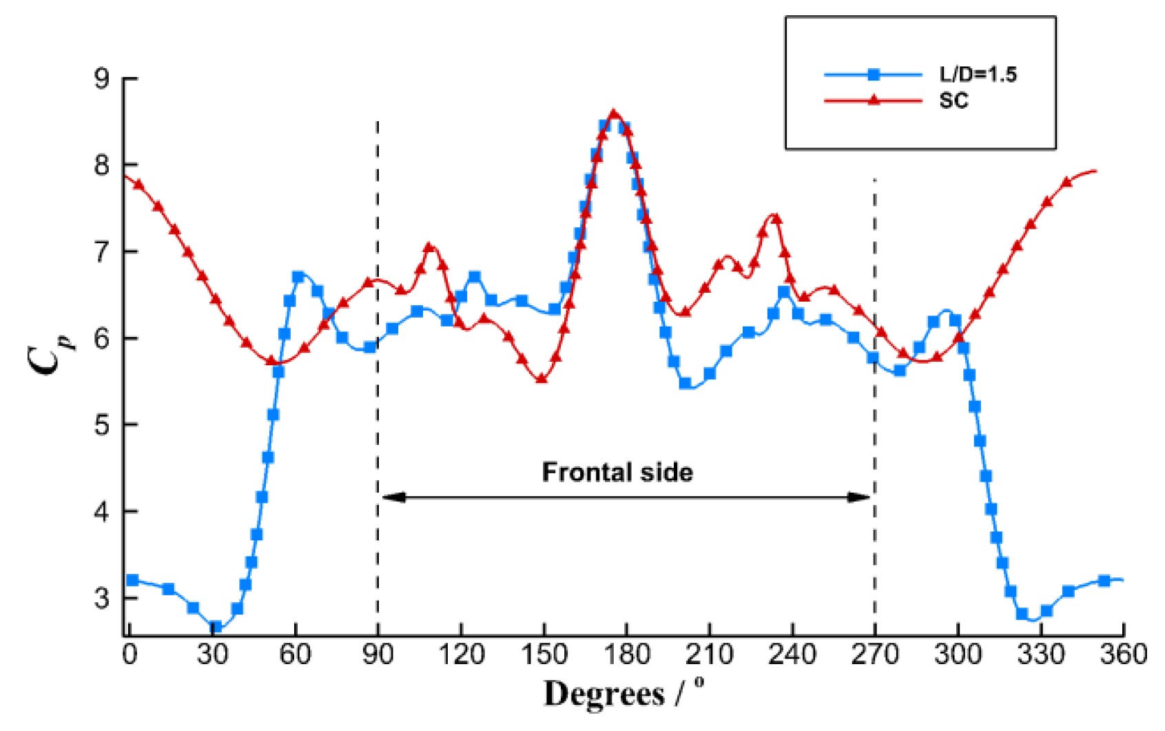
From the pressure distribution diagram shown in Figure 17, the presence of P2 causes the lee side of P1 to be submerged in an area of low pressure. The vortices between the two cylinders are suppressed, significantly reducing the pressure on the lee side of P1. On the other hand, the pressure on the frontal side of P1 changes slightly. As a result, acting on P1 in the positive direction increases. This explains why acting on P1 is larger than that on the SC (as shown in Figure 15) in the lower layer.
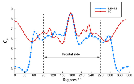
Figure 17.
Pressure distribution comparison diagram of SC and P1 (Y = 0.16 m), L/D = 1.5.
4.2.2. Distinction of the Flow Field and Pressure Distribution between P1 and SC (2.0 ≤ L/D ≤ 3.0)
As shown in Figure 14, the maximum on P1 occurs at L/D = 1.5, and it gradually decreases with increasing L/D. When L/D ≥ 3.0, the forces on P1 approach those on the SC. Therefore, a comparison between P1 at L/D = 2, L/D = 2.5, L/D = 3.0, and SC is conducted to explore the corresponding mechanical characteristics and flow field.
The comparison of the vertical distribution of on P1 in the SC, L/D = 2, L/D = 2.5, and L/D = 3.0 is illustrated in Figure 18. For L/D = 2.0, L/D = 2.5, and L/D = 3.0, the upper parts of the cylinder exhibit a slightly smaller than the SC. However, on the lower parts of the cylinder are significantly greater than those on the SC. As a result, the horizontal resultant force acting on P1 is greater than that on the SC.
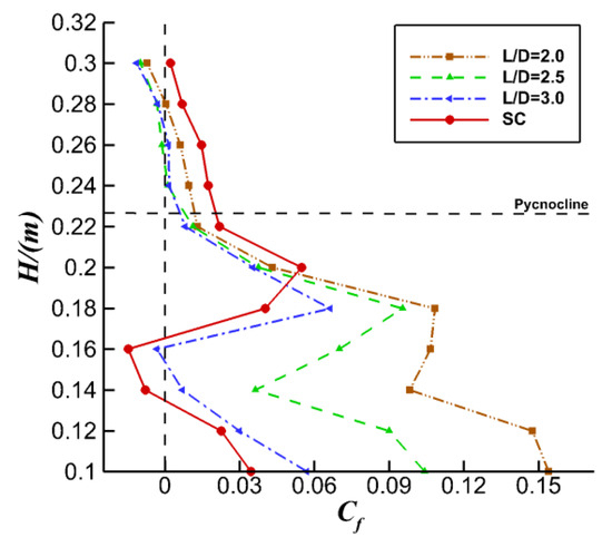
Figure 18.
Vertical distribution of comparison diagram of SC and P1 (CFn = CFn−max), L/D = 2.0, 2.5, 3.0.
Similarly, the flow field and pressure distribution at Y = 0.16 m are illustrated in Figure 19 and Figure 20, respectively. Compared to the SC, with increasing L/D from 2.0 to 3.0, the suppression of vortices between the two cylinders gradually diminishes (see Figure 19), and the pressure distribution around the circumference of P1 gradually returns to a state similar to that of the SC (see Figure 20). Therefore, when 2.0 ≤ L/D ≤ 3.0, the differences in forces on the cylinder are also evident in the lower layer, mainly concentrated in the 0°–30° and 330°–360° sections of the cylinder circumference.

Figure 19.
Flow field characteristics comparison diagram (Y = 0.16 m). (a) SC, (b) L/D = 2.0, (c) L/D = 2.5, (d) L/D = 3.0.
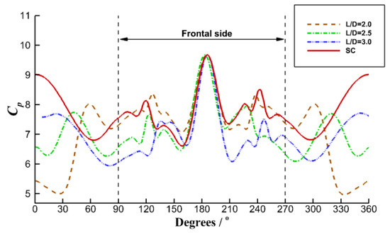
Figure 20.
Pressure distribution comparison diagram of SC and P1 (Y = 0.16 m), L/D=2.0, 2.5, 3.0.
4.2.3. Distinction of the Flow Field and Pressure Distribution between P1 and SC (3.0 < L/D ≤ 6.0)
As shown in Figure 21, when L/D > 3.0, the values on the upper and lower parts of P1 are both similar to those on the SC. Therefore, if L/D is larger than Lc/D, then the mutual interference between the two cylinders gradually transitions to an undisturbed state, and the flow field and circumferential pressure distribution around the two cylinders gradually return to a state similar to that of SC. Consequently, further discussion on the flow field and pressure distribution characteristics is not necessary.
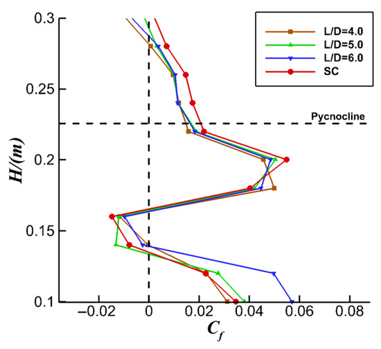
Figure 21.
Vertical distribution of comparison diagram of SC and P1 (CFn = CFn−max), L/D = 4.0, 5.0, 6.0.
In conclusion, the size and location of the vortex region are determined by L/D, evidently affecting the forces acting on P1. Figure 15, Figure 18 and Figure 21 show that the presence of P2 has a significant impact on the forces acting on P1 when L/D < Lc/D, with the force differences mainly manifesting in the lower layer.
4.3. Effects of L/D on the Force Behaviors and Flow Field Characteristics for P2
Similarly, when ηo/H = 0.057, the duration curves of for P2 under different L/D cases (1.5 ≤ L/D ≤ 6) are shown in Figure 22. on P2 varies significantly over time. When L/D ≥ 3, the overall trend of the curves for P2 is similar to that of the SC, although the on the SC is slightly larger than that of L/D ≥ 3. However, when 1.5 ≤ L/D ≤ 2, P2 experiences a larger negative (opposite to the wave propagation direction), and the on P2 is negative. By employing the same analysis method as that for P1, the comparison of the flow field and pressure distribution between the SC and P2 at different L/D cases is shown to reveal the force characteristics of P2 in an IW environment. The specific cases are detailed in Table 4.

Figure 22.
Comparison of the duration curves of for different cases for P2.
Table 4.
Simulation cases for studying the forces acting on P2.
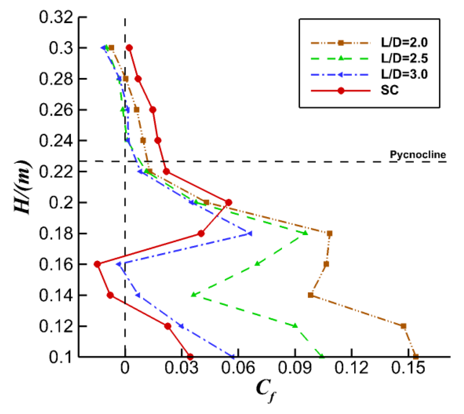
Figure 23 illustrates the vertical distribution of for P2 at different L/D cases. When 1.5 ≤ L/D < 3.0, the upper parts of P2 experience significantly smaller forces compared to the SC. However, in the lower layer, the situation is reversed, and the lower parts of P2 suffer significantly higher forces than those of the SC. When 3 ≤ L/D ≤ 6.0, the forces on the upper parts of P2 are similar to those on the SC, but the forces on the lower parts are significantly higher. Therefore, the investigation of the forces on P2 primarily focuses on the flow field and pressure distribution characteristics in the upper layer for 1.5 ≤ L/D < 3.0 and in the lower layer for 1.5 ≤ L/D ≤ 6.
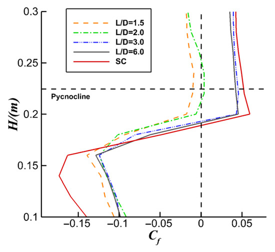
Figure 23.
Vertical distribution of comparison diagram of SC and P2 (CFn = CFn−max).
4.3.1. Distinction of the Flow Field and Pressure Distribution in the Upper Layer between P2 and SC (1.5 ≤ L/D < 3.0)
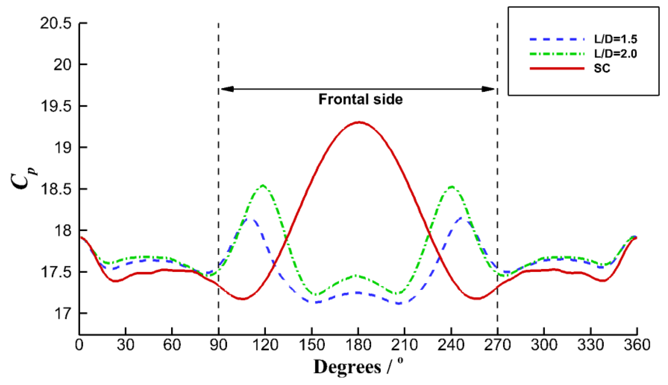
Figure 24a–c presents the flow field contour maps. It can be observed that when 1.5 ≤ L/D < 3.0, the frontal side of P2 is immersed in a low-pressure vortex area, significantly reducing the pressure on the frontal side of P2 (see Figure 25). Clearly, the pressure on the frontal side of P2 is significantly lower than that on the SC. Consequently, the pressure on the frontal side of P2 is lower than that on the lee side, compelling the forces on P2 to be negative.
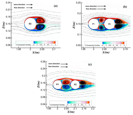
Figure 24.
Flow field characteristics comparison diagram (Y = 0.26 m). (a) SC, (b) L/D = 1.5, (c) L/D = 2.0.
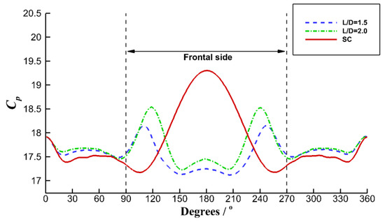
Figure 25.
Pressure distribution comparison diagram of SC and P2 (Y = 0.26 m).
4.3.2. Distinction of the Flow Field and Pressure Distribution in the Lower Layer between P2 and SC (1.5 ≤ L/D ≤ 6)
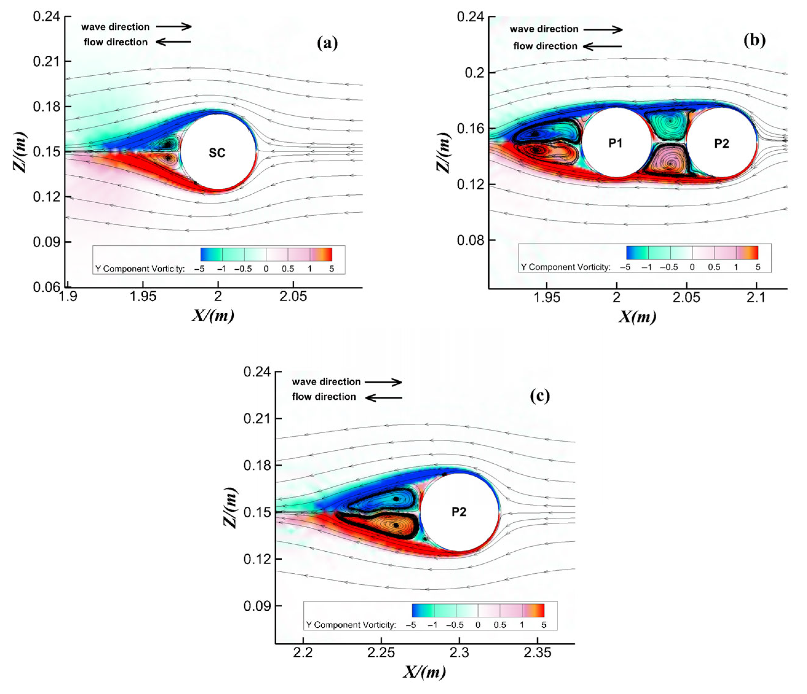
The comparison of the flow field in Figure 26a,b shows that when L/D = 1.5, the frontal side of P2 is still immersed in vortices, resulting in lower pressure on the frontal side than on the SC (as shown in Figure 27). When L/D = 6.0, the development of vortices in front of P2 still differs significantly from the SC (as observed by comparing Figure 26a,c). As a result, the pressure on the frontal side of P2 remains lower than that on the SC (as shown in Figure 27). This explains why, when L/D ≥ 3, the overall force trend of P2 is similar to that of the SC, but on P2 is slightly smaller than that on the SC (as shown in Figure 22).

Figure 26.
Flow field characteristics comparison diagram (Y = 0.16 m). (a) SC, (b) L/D = 1.5, (c) L/D = 6.0.
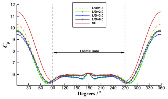
Figure 27.
Pressure distribution comparison diagram of SC and P2 (Y = 0.16 m).
To summarize, the size and position of the vortex region are significantly determined by L/D, directly affecting the forces acting on P2. Combining the observations from Figure 24, Figure 25, Figure 26 and Figure 27, it can be concluded that for 1.5 ≤ L/D < 3.0, the differences in forces between P2 and the SC are primarily determined by the pressure differences on the frontal side in the upper layer and the lee side in the lower layer. For 3 ≤ L/D ≤ 6, the differences in forces between P2 and the SC are primarily determined by the pressure differences on the lee side in the lower layer.
5. Discussion
(1) It should be noted that the LES (large eddy simulation) method used in this study has some level of uncertainties in terms of accuracy compared to the direct numerical simulation (DNS) method, particularly in the context of low to moderate Reynolds numbers. In future research, the DNS method should be employed specifically for cases involving these Reynolds numbers.
(2) We carried out the grid independent analysis, with grids having (low density) 525,454, (moderate density) 2,384,640, and (high density) 3,318,278 grid points. In future research, more thorough grid refinement studies will be conducted, such as adjusting the grid number with medium density to eight times that of low density, and further increasing the grid number difference between high grid density and medium grid density.
(3) The corresponding Reynolds number of the IWs environment is calculated in this paper. The Reynolds number is typically quite small, usually on the order of 103, which is consistent with the Reynolds numbers found in the relevant studies by Terletska [28], Harnanan [29], Hsieh [30], Arthur [31], and Sutherland [32], all of which are at laboratory scales. Due to limitations in computational resources, a grid quantity of 3,318,278 (chosen for the high-density case of the grid independent analysis) is essentially the computational limit for our current study, requiring approximately 130 h of computation on a quad-core CPU.
In our future research, we will also make every effort to secure funding for the purchase of more powerful computers to further refine our model and grid.
6. Conclusions
This study investigates the force characteristics of two tandem cylinders in the presence of an IW environment over slope terrain using a three-dimensional numerical wave tank. By analyzing the force duration curves, vorticity contour maps, flow field distributions, and pressure distribution maps, the study provides a detailed understanding of the force responses of P1 and P2 for different L/D cases. The conclusions are described as follows:
(1) When IWs interact with the slope terrain, the flow field around the cylinders becomes more complex and dynamic, leading to a significant alteration of the force characteristics. The horizontal force acting on the cylinder over the slope is opposite to that action on the cylinder without the slope, with the interaction between IWs and topography playing a crucial role. Bounded by the pycnocline, the impact of the topography on the forces is mainly observed on the lee side of the upper parts and the frontal side of the lower parts of the cylinders.
(2) The dimensionless spacing between the cylinders (L/D) has a significant influence on the forces on P1 and P2. A critical spacing, defined as Lc/D = 3.0, is identified to differentiate between strong and weak interference regimes. In the strong interference regime (L/D ≤ Lc/D), P1 and P2 experience larger forces in the downstream and upstream directions, respectively. In the weak interference regime (L/D > Lc/D), the force responses of P1 and P2 gradually close to those of an SC, but with slightly lower maximum forces. The effects of spacing are predominantly observed in the lower parts of the cylinders.
(3) The pressure distribution and flow field characteristics around the cylinders reveal the mutual disturbance mechanism between P1 and P2 under the coupling effect of IWs and slope topography. L/D determines the size and location of the vortex region, directly influencing the force characteristics of the cylinders. The vortex disturbance in the lower layer is more pronounced. When L/D ≤ Lc/D, the influence of the vortexes in the upper layer on the force on the cylinder can be ignored. The presence of P2 significantly affects the forces on P1, with a difference from the forces on the SC primarily observed in the flow field and pressure distribution in the lower layer. Similarly, the presence of P1 also significantly influences the forces on P2, with differences from the forces on the SC manifested in both the upper and lower layers in terms of the flow field and pressure distribution.
Author Contributions
Writing—original draft, Y.W.; writing—review and editing, X.X. and C.Z.; conceptualization, L.W. and C.W.; validation, X.W., H.W. and Z.L. All authors have read and agreed to the published version of the manuscript.
Funding
This study was partially supported by the National Natural Science Foundation of China (Grant Nos. 52109090, 52009087, and 51879086), the China Postdoctoral Science Foundation Funded Project (Grant No. 2022M721426).
Data Availability Statement
The data that support the findings of this study are available from the corresponding author upon reasonable request.
Conflicts of Interest
The authors declare no conflict of interest.
References
- Kurkina, O.; Rouvinskaya, E.; Talipova, T.; Soomere, T. Propagation regimes and populations of internal waves in the Mediterranean Sea basin. Estuar. Coast. Shelf Sci. 2017, 185, 44–54. [Google Scholar] [CrossRef]
- Cheng, S.Y.; Yu, Y.; Li, Z.M.; Huang, Z.X.; Zhang, X.M.; Yu, J.X. Research on dynamic response of deep-water semi-submersible platform system under internal solitary wave. Ocean Eng. 2022, 40, 123–138. (In Chinese) [Google Scholar]
- Wang, X.; Lin, Z.Y.; You, Y.X.; Yu, R. Numerical Simulations for the Load Characteristics of Internal Solitary Waves on a Vertical Cylinder. Chuan Bo Li Xue/J. Ship Mech. 2017, 21, 1071–1085. [Google Scholar]
- Cai, S.; Long, X.; Wang, S. Forces and torques exerted by internal solitons in shear flows on cylindrical piles. Appl. Ocean Res. 2008, 30, 72–77. [Google Scholar] [CrossRef]
- Yang, F.; Zhu, R.Q.; Chen, X.D.; Ji, R.W.; Liu, X. Numerical simulation for the load of internal solitary waves acting on a submerged body. Ship Sci. Technol. 2017, 39, 26–31. (In Chinese) [Google Scholar]
- Wang, L.L.; Wang, Y.; Wei, G.; Lu, Q.Y.; Xu, J.; Tang, H.W. Force behaviors of circular and square cylinder in internal solitary waves environment–I. Experimental investigation. Adv. Water Sci. 2017, 28, 429–437. (In Chinese) [Google Scholar]
- Wang, L.L.; Wang, Y.; Wei, G.; Lu, Q.Y.; Xu, J.; Tang, H.W. Force behaviors of circular and square cylinder in internal solitary waves environment—II. Numerical study. Adv. Water Sci. 2017, 28, 588–597. (In Chinese) [Google Scholar]
- Helfrich, K.R. Internal solitary wave breaking and run-up on a uniform slope. J. Fluid Mech. 1992, 243, 133–154. [Google Scholar] [CrossRef]
- Timothy, W. Internal solitons on the pycnocline: Generation, propagation, and shoaling and breaking over a slope. J. Fluid Mech. 1985, 159, 19–53. [Google Scholar]
- Chen, C.Y.; Hsu, J.; Chen, H.H.; Kuo, C.F.; Cheng, M.H. Laboratory observations on internal solitary wave evolution on steep and inverse uniform slopes. Ocean Eng. 2007, 34, 157–170. [Google Scholar] [CrossRef]
- Colosi, J.A.; Kumar, N.; Suand, A.S.H.; Freismuth, T.M.; MacMahan, J.H. Statistics of internal tide bores and internal solitary waves observed on the inner continental shelf off point sal CA. J. Phys. Oceanogr. 2018, 48, 123–143. [Google Scholar] [CrossRef]
- Liapidevskii, V.; Gavrilov, N. Large internal solitary waves in shallow waters. In The Ocean in Motion; Springer: Cham, Switzerland, 2018; pp. 87–108. [Google Scholar]
- Zdravkovich, M.M. Review of flow interference between two circular cylinders in various arrangements. J. Fluids Eng. 1977, 99, 618–633. [Google Scholar] [CrossRef]
- Gopalan, H.; Jaiman, R. Numerical study of the flow interference between tandem cylinders employing non-linear hybrid URANS–LES methods. J. Wind. Eng. Ind. Aerodyn. 2015, 142, 111–129. [Google Scholar] [CrossRef]
- Alam, M.M.; Zhou, Y. Strouhal numbers, forces and flow structures around two tandem cylinders of different diameters. J. Fluids Struct. 2008, 24, 505–526. [Google Scholar] [CrossRef]
- Meneghini, J.R.; Saltara, F.; Siqueira, C.; Ferrari, J.A., Jr. Numerical simulation of flow interference between two circular cylinders in tandem and side-by-side arrangements. J. Fluids Struct. 2001, 15, 327–350. [Google Scholar] [CrossRef]
- Wang, Y.; Wang, L.; Ji, Y.; Zhang, J.; Xu, M.; Xiong, X.; Wang, C. Research on the force mechanism of two tandem cylinders in a stratified strong shear environment. Phys. Fluids 2022, 34, 053308. [Google Scholar] [CrossRef]
- Germano, M.; Piomelli, U.; Moin, P.; Cabot, W.H. A dynamic subgrid-scale eddy viscosity model. Phys. Fluids A 1991, 3, 1760–1765. [Google Scholar] [CrossRef]
- Lin, Z.H.; Song, J.B. Numerical studies of internal solitary wave generation and evolution by gravity collapse. J. Hydro-Dyn. 2012, 24, 541–553. [Google Scholar] [CrossRef]
- Tolias, I.C.; Kanaev, A.A.; Koutsourakis, N.; Glotov, V.Y.; Venetsanos, A.G. Large Eddy Simulation of low Reynolds number turbulent hydrogen jets - Modelling considerations and comparison with detailed experiments. Int. J. Hydrog. Energy 2020, 46, 12384–12398. [Google Scholar] [CrossRef]
- Bailly, B.C. Large eddy simulations of round free jets using explicit filtering with/without dynamic Smagorinsky model. Int. J. Heat Fluid Flow 2006, 27, 603–610. [Google Scholar]
- Zhu, H.; Wang, L.L.; Tang, H.W. Large-eddy simulation of the generation and propagation of internal solitary waves. Sci. China 2014, 57, 1128–1136. [Google Scholar] [CrossRef]
- Zhu, H.; Lin, C.; Wang, L.L.; Kao, M.; Tang, H.; Williams, J.J.R. Numerical investigation of internal solitary waves of elevation type propagating on a uniform slope. Phys. Fluids 2018, 30, 116602. [Google Scholar] [CrossRef]
- Li, X.; Ren, B.; Wang, G.Y.; Wang, Y.X. Numerical simulation of hydrodynamic characteristics on an arc crown wall using volume of fluid method based on BFC. J. Hydrodyn. 2011, 23, 767–776. [Google Scholar] [CrossRef]
- Chen, Y. Flow simulation of car air conditioner duct based on SIMPLE algorithm. Mech. Eng 2008, 11, 111–112. [Google Scholar]
- Wang, F. Study on Hydrodynamic Characteristics of Small Scale Vertical Cylinders under Internal Solitary Wave; Ocean University of China: Qingdao, China, 2015. (In Chinese) [Google Scholar]
- Chen, C.Y.; Hsu JR, C.; Chen, C.W.; Chen, H.H.; Kuo, C.F.; Cheng, M.H. Generation of internal solitary wave by gravity collapse. J. Mar. Sci. Technol. 2007, 15, 1. [Google Scholar] [CrossRef]
- Terletska, K.; Jung, K.T.; Talipova, T.; Maderich, V.; Brovchenko, I.; Grimshaw, R. Internal breather-like wave generation by the second mode solitary wave interaction with a step. Phys. Fluids 2016, 28, 116602. [Google Scholar] [CrossRef]
- Harnanan, S.; Stastna, M.; Nancy, S. The effects of near-bottom stratification on internal wave induced instabilities in the boundary layer. Phys. Fluids 2017, 29, 016602. [Google Scholar] [CrossRef]
- Hsieh, C.M.; Cheng, M.H.; Hwang, R.R.; Hsu, J.R.C. Numerical study on evolution of an internal solitary wave across an idealized shelf with different front slopes. Appl. Ocean Res. 2016, 59, 236–253. [Google Scholar] [CrossRef]
- Arthur, R.S.; Fringer, O.B. The dynamics of breaking internal solitary waves on slopes. Fluid Mech. 2014, 761, 360–398. [Google Scholar] [CrossRef]
- Sutherland, B.R.; Barrett, K.J.; Ivey, G.N. Shoaling internal solitary waves. J. Geophys. Res. Ocean. 2013, 118, 4111–4124. [Google Scholar] [CrossRef]


Disclaimer/Publisher’s Note: The statements, opinions and data contained in all publications are solely those of the individual author(s) and contributor(s) and not of MDPI and/or the editor(s). MDPI and/or the editor(s) disclaim responsibility for any injury to people or property resulting from any ideas, methods, instructions or products referred to in the content. |
© 2023 by the authors. Licensee MDPI, Basel, Switzerland. This article is an open access article distributed under the terms and conditions of the Creative Commons Attribution (CC BY) license (https://creativecommons.org/licenses/by/4.0/).