Abstract
Ecological flow (E-flow) determination is an essential component of stream management and the preservation of aquatic ecosystems within a watershed. E-flow should be determined while considering the overall status of the watershed, including the hydrological cycle, hydraulic facility operation, and stream ecology. The purpose of this study is to determine E-flow by considering watershed status through coupled modeling with SWAT and PHABSIM. SWAT was calibrated to ensure reliability when coupling the two models, using observed data that included streamflow and dam inflows. The calibration result of SWAT showed that the averages of R2, NSE, and RMSE were 0.62, 0.57, and 1.68 mm/day, respectively, showing satisfactory results. Flow duration analysis using the SWAT results was performed to apply to discharge boundary conditions for PHABSIM. The averages of Q185 (mid-range flows) and Q275 (dry conditions) were suitable to simulate fish habitat. The habitat suitability index derived through a fish survey was applied to PHABSIM to estimate E-flow. E-flow was estimated at 20.0 m3/s using the coupled model and compared with the notified instream flow by the Ministry of Environment. The results demonstrate a high level of applicability for the coupled modeling approach between the watershed and physical habitat simulation models. Our attempt at coupled modeling can be utilized to determine E-flow considering the watershed status.
1. Introduction
In 1999, South Korea amended its river laws, shifting the focus towards water conservation, regulation, and the protection of the environment and ecology during their development. This led to an increase in the utility of rivers, but it also resulted in direct harm to the river environment due to the construction of hydraulic facilities such as dams and reservoirs. This construction had a significant impact on the habitat of aquatic organisms [1]. The climate change that has occurred since 1999 has also led to changes in precipitation patterns, resulting in increased variability in water resources. Furthermore, the ongoing construction of hydraulic facilities has posed a further threat to the health of the aquatic ecosystem [2,3,4].
Aquatic ecosystems, which are composed of organisms living in rivers, are highly responsive to changes in water quantity and quality [5,6,7]. The response of aquatic organisms to disturbances, such as changes in streamflow and water quality, can be used as an indicator [8]. To manage and conserve these ecosystems, many countries have been estimating the ecological flow (E-flow) using various methods. Generally, E-flow can be defined as the minimum flow that must be maintained in a stream to ensure that existing ecosystems thrive under appropriate hydrological and environmental conditions that respect the ecological balance [9]. The methods of estimating E-flow are classified as the hydrological method, hydraulic method, hydraulic rating method, habitat simulation method, and holistic method [5]. Among these, the habitat simulation method is widely used. The hydrological method was also widely used and is suitable for water resources planning; however, it is non-stationary and lacks considerations of actual habitat requirements [10]. The hydraulic method is easier than other methods and does not require detailed aquatic ecosystem data, but it lacks an objective approach [11]. The holistic method considers physical, ecological, and socio-cultural aspects, but it is expensive to implement continuously and relies on the subjective opinions of experts [12]. The habitat simulation method is considered the most scientifically and legally defensible approach for E-flow, and it helps clarify hydrological–ecological relationships [13,14]. The estimation of E-flow using the habitat simulation method involves a combination of field surveys and modeling. The modeling process typically includes the analysis of fish habitats using physical habitat models to manage water resources and aquatic ecosystems, as outlined in the physical habitat modeling approach described in [15]. By modeling fish habitats, it is possible to estimate the minimum flow required to maintain good conditions for aquatic organisms based on the hydrological and environmental conditions. The physical habitat simulation system (PHABSIM) is a widely used model for estimating E-flow by analyzing fish habitats [16,17,18]. In particular, K-water, a public corporation responsible for managing water resources in South Korea, utilizes PHABSIM to quantitatively manage E-flow [19].
Globally, stream environments and aquatic ecosystems have been managed using E-flow through various methods. India has primarily managed E-flow using the hydrological method to ensure water security [20]. However, India, like South Korea, is still in the early development phase. India defines E-flow as the natural or regulated flow of a specific quantity, timing, duration, frequency, and quality of streamflow required to manage the ecological system, including the sustainability of freshwater, estuarine, and near-shore ecosystems [20,21]. Japan has managed E-flow using the hydraulic method for 30 years, and this is regulated by national law [22]. In Europe, especially in Mediterranean regions including Spain, Greece, Italy, Portugal, France, Cyprus, and Malta, E-flow has been determined using various methods considering each country’s characteristics to conserve non-perennial rivers. Among the methods used in each country, the most used methods were determined to be the hydrological method and the habitat simulation method [14].
However, a stream is influenced by the hydrologic cycle in the watershed, and its influence affects the aquatic ecosystem and habitat. Physically based habitat models can easily estimate E-flow through the hydrological–ecological relationship, but streamflow is highly variable in space and time [23,24] and affected by operations from hydraulic facilities such as dams, reservoirs, and sewage treatment plants. The European Commission [25] has emphasized that when setting E-flow, it should be done considering all components of the natural watershed, as well as the relationships between hydrology, ecology, and morphological aspects. In the past, instream flow (IF) and E-flow have been regarded the same concept. However, now that E-flow is encompassed within the concept of IF, it should be estimated considering the overall watershed status including the hydrologic cycle, operation at hydraulic facilities, and so on. To complement these points, one needs to link habitat model with a model that can simulate long-term streamflow and consider overall watershed status.
The Soil and Water Assessment Tool (SWAT), a semi-distributed long-term simulation model, is globally applied to gain insights into hydrology-driven ecological processes, and it can be used as an ecohydrological model [26,27,28]. The reason SWAT can play this role is because it can consider the overall watershed status. SWAT is basically composed of land use/cover and soil maps, and it can help to operate reservoir and sewage treatment plants. There are many studies that link SWAT with other models using these advantages, but there are few studies about its linkage with PHABSIM. Ref. [29] tried to generate PHABSIM input data by applying SWAT results and found that SWAT, which uses a high-resolution digital elevation model (DEM), is suitable for coupling with PHABSIM. In this way, the mode of coupled modeling between two models is sufficiently suitable, and if the advantages of SWAT are utilized and coupled with PHABSIM, E-flow will be able to be estimated considering the overall watershed status.
The main objectives of this study are: (1) to perform coupled modeling between SWAT and PHABIM using the flow duration results of SWAT, and (2) to determine the optimal E-flow considering overall watershed status.
2. Data and Methods
2.1. Study Area
South Korea has five major rivers. Among the five major rivers, the Nakdong River has the poorest water quality and aquatic ecosystem compared to the other major rivers. Water management issues in this basin include high rates of water pollution, including algal bloom [30], and a lack of E-flow for aquatic ecosystem. Based on these issues, the South Korea Dam Operation Council has implemented partial releases for certain dams in the Nakdong River [31]. Andong (ADD) and Imha (IHD) dams are located upstream of the Nakdong River in the southeastern area of South Korea (Figure 1a). The Gudam upstream basin (GDUB) area is 4584.8 km2 with a target stream length of 410.0 m (Figure 1b). The Gudam wetland located downstream of ADD and IHD is composed of many sand bars, and so it has ecological value as it is used as a habitat for various aquatic organisms. The watershed outlet of GDUB has a Gudam streamflow gauging station (GD) (Figure 1c) and an IF notification spot named Jibo (JB), which is managed by the Ministry of the Environment (ME) in South Korea. The annual average temperature and precipitation in the study area were 11.8 °C/year and 1072.3 mm/year, respectively, over the past 40 years (1981 to 2020). Table 1 shows the characteristics of the target stream and streamflow gauging station investigated by the Ministry of Land, Infrastructure and Transport in South Korea (MOLIT) [32].
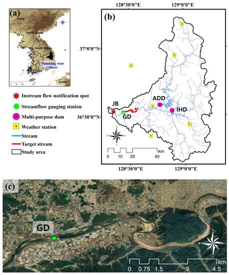
Figure 1.
(a) The location of the study area, (b) description of the study area showing the locations of observation stations (streamflow gauging, and weather), IF notification spot, target stream, and two multi-purpose dams (ADD and IHD), and (c) satellite images of target stream for estimating E-flow using PHABSIM modeling.

Table 1.
Characteristics of the target stream investigated by MOLIT for the fish habitat study.
2.2. Dataset
The data include geographic information system (GIS) spatial data, meteorological data, hydrological data (such as dam inflow, dam release, and streamflow), and field survey data of the target stream. GIS spatial and meteorological data were mainly used for SWAT. Hydrological data were used for model calibration and validation.
In this study, 30 m-spatial resolution DEM, 1:25,000 precision land use, and soil textures were used to compose the SWAT. The average elevation of the study area is 407.4 m (Figure 2a). The forest cover is 77.3%, and rice paddy and upland crop areas occupy 16.2% (Figure 2b). Silt loam and loam are the dominant soil types, representing 47.4% and 20.8%, respectively (Figure 2c).
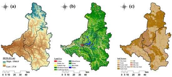
Figure 2.
GIS spatial data: (a) DEM, (b) land use, and (c) soil textures.
In total, 46 years (1975–2020) of daily meteorological data, including precipitation (mm), maximum and minimum temperature (°C), wind speed (m/s), relative humidity (%), and solar radiation (MJ/m2), were collected from 6 weather stations (Figure 1) for SWAT modeling.
For PHABSIM modeling, the field survey data for the target stream included water depth, velocity, stream topographic, and discharge. The hydraulic data, including cross-section data of the target stream, were provided by MOLIT [32]. The field survey and cross-section data were used in PHABSIM modeling.
The field survey was conducted intensively during the dry season when the streamflow was at its lowest point throughout the year. The fish survey was conducted 4 times on 26 March, 26 April, 15 May, and 3 June 2021. There is a weir operating in the upstream area of GD, making it unsuitable for use in the fish survey. Therefore, the fish survey was conducted downstream of GD near to JB with similar river and physical characteristics. Fish were collected from the downstream area of GD using casting nets and skimming nets. Field data regarding the physical habitat of the survey location, as well as water depth, velocity, and bed materials, were recorded.
Figure 3 shows the results of the fish and physical habitat surveys undertaken in the field. The casting nets were applied more than 10 times in riffles and pools inhabited by various fish. The skimming nets were used under the rock and at the waterfront. For substrate assessment, the size of the bed material was measured using a 50 by 50 cm quadrat. The substrate structure was calculated as the area ratio. In this study, the 8 sets of cross-sectional topographic data of the target stream were taken at intervals of about 51.1 m, and the hydraulic data provided by [32] were used to generate the hydraulic input data for PHABSIM.
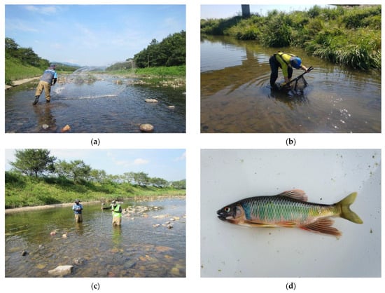
Figure 3.
Description of fish and physical habitat monitoring in field: (a) casting net, (b) skimming net, (c) investigation of depth and velocity, and (d) fish (Zacco platypus) collected in the field.
2.3. Hydrological Modeling
Using the data, PHABSIM was constructed and coupled with SWAT (Figure 4). To reduce uncertainty when linking the models, it is important to ensure reliability by verifying the models using objective functions. SWAT was calibrated (2012–2016) and validated (2017–2020) using the daily observed dam inflow (ADD and IHD) and streamflow (GD) data. The calibration and validation were performed manually using a trial-and-error approach based on physically realistic parameter ranges reflecting the study area’s characteristics.
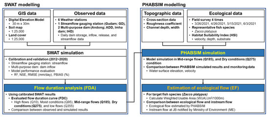
Figure 4.
Flowchart of the study.
The statistical performance of SWAT was assessed using various objectives, such as the coefficient of determination (R2), the Nash–Sutcliffe model efficiency (NSE), the percent bias (PBIAS), the root mean square error (RMSE), and others. R2 is used to assess the proportion of the variance between the observed and simulated values. It has a value between 0 and 1, where an R2 of 1 indicates perfect model simulation, with no deviation from the observed values. NSE represents the efficiency of the model by comparing the relative magnitude of the residual variance with the variance of the measured data [33]. NSE has a range of −∞ to 1, and the model’s simulation output is considered better than the mean of observed values when the NSE is greater than zero. PBIAS means the average tendency of the values of the simulated data to be greater than or less than the values of the observed data. A negative value of PBIAS indicates the model’s results are overestimated compared to the observed data, while a positive value of PBIAS indicates that the model’s results were underestimated [34]. In particular, a PBIAS value of zero indicates perfect model simulation. RMSE refers to the statistical error between the observed and simulated values as the standard deviation of the residual [35].
For PHABSIM modeling, the calibrated streamflow of SWAT was used to determine discharge boundary conditions. The initial boundary conditions of the water surface’s elevation and velocity were established using the calibrated streamflow of the target stream and cross-section data. Normal and dry boundary conditions, derived from the flow duration analysis (FDA) results for nine years (2012–2020), were applied to estimate the E-flow.
2.3.1. SWAT Description
SWAT is a watershed-scale continuous hydrological model developed by the United States Department of Agriculture–Agricultural Research Services (USADA-ARS) to evaluate the impact of water resources, water quality, and agricultural chemicals on various soil characteristics, land use and management conditions [36,37]. SWAT can simulate the overall hydrologic and nutrient cycles, including evapotranspiration, surface runoff, later flow, base flow, groundwater flow, soil erosion, and nutrients transport, under the various watershed environmental conditions for each of the hydrologic response units (HRUs) based on the water balance equation [38]. The theories of SWAT are elaborated in [38].
2.3.2. PHABSIM Description
PHABSIM was developed to support and establish E-flow, IF, and water resource management. PHABSIM consists of two subsystems, namely, hydraulic and habitat models. These two subsystems provide a variety of simulation tools, which characterize the physical microhabitat structure of a stream and describe the flow-dependent characteristics of the physical habitat in the light of selected biological responses of target species and life stages [39].
PHABSIM can simulate hydraulic relationships at various streamflows using water surface elevations, velocities, and substrates for each cross-section [39]. It quantifies the hydraulic relationship and parameters (water depth, velocity, and substrate) related to habitat suitability for target species. PHABSIM is calibrated using measured hydraulic parameters, and it then estimates the same physical habitat parameters for other discharges.
PHABSIM analyzes the physical habitat changes of the target species based on species and life stages according to changes in the streamflow, water depth, and velocity of the stream. Subsequently, PHABSIM estimates the weighted usable area (WUA) based on the Instream Flow Incremental Method (IFIM) for each discharge by increasing the streamflow, and defines the streamflow when the WUA is maximum as the optimal E-flow [16,39,40]. WUA is calculated by multiplying the area of cells and the HSI. The equation is expressed as:
where WUA is the weighted usable area at a specified discharge, Ai is the area of cell i, and Ci is the combined suitability of cell i.
The combined suitability of the cell is derived from the component attributes of each cell, which are evaluated against the species and life stage habitat suitability coordinates for each attribute to derive the component suitability. The combined suitability is calculated as follows:
where Ci is the combined suitability of cell i, Vi is the velocity suitability in cell i, Di is the depth suitability in cell i, and Si is the substrate suitability in cell i.
3. Results
3.1. SWAT Calibration and Validation
SWAT was calibrated for 5 years (2012–2016) and validated for 4 years (2017–2020) to assess its capability to simulate the watershed hydrology of the GDUB. The SWAT was adjusted to have 10 parameters for simulating the watershed hydrology. The adjusted parameters are SCS curve number, Manning’s “n” value, effective hydraulic conductivity, soil evaporation compensation coefficient, maximum canopy storage, available water capacity of the soil layer, saturated hydraulic conductivity, delay time for aquifer recharge, threshold water level in shallow aquifer, and base flow recession constant (Table 2). For operating two multi-purpose dams, the five parameters related to hydraulic facilities’ specification were adjusted.
Table 2.
The adjusted parameter lists for SWAT calibration.
The calibration and validation results are summarized in Table 3 and Figure 5. The average R2 values of ADD, IHD, and GD were 0.74, 0.61, and 0.52, respectively. The average NSE values of ADD, IHD, and GD were 0.74, 0.61, and 0.52, respectively. The average RMSE values of ADD, IHD, and GD were 1.62 mm/day, 2.51 mm/day, and 0.92 mm/day, respectively. The average PBIAS values of ADD, IHD, and GD were −14.9%, −32.1%, and −2.7%, respectively. Unlike the results of ADD, the statistical results of IHD were assessed as relatively poor. The annual average precipitation during calibration and validation periods of IHD was 947.8 mm/year, which is lower than the annual average precipitation of the watershed. Especially, in 2013, 2015, and 2017, the annual average precipitation levels were 839.0 mm/year, 606.8 mm/year, and 732.2 mm/year, respectively, representing drought periods. These droughts influenced the overall statistical calibration and validation results, and the error caused by the droughts continued to the end of the validation periods. At the GD station, the average values of R2 and NSE were assessed as relatively poorer than those of two multi-purpose dams. The observed streamflow data of GD in 2016 and 2018 are missing. In addition, the average annual runoff ratios for the observed and simulated values are 37.1% and 35.9%, respectively.
Table 3.
Calibration and validation results for SWAT dam inflows and streamflow during 2012–2020.
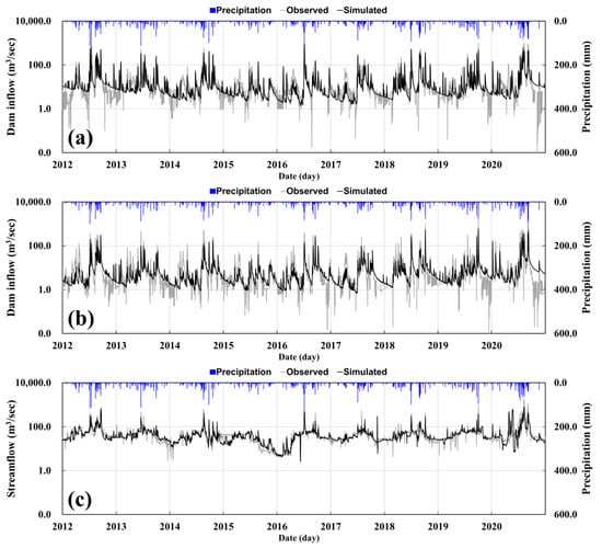
Figure 5.
Comparison of daily observed and simulated dam inflows and streamflow during 2012–2020: (a) ADD, (b) IHD, and (c) GD.
3.2. Flow Duration Analysis Based on the SWAT Simulation Result
The FDA was performed to determine the discharge boundary condition for PHABSIM using both observed and SWAT calibrated data from GD during 2012–2020. The FDA can analyze temporal changes in the streamflow at a point in the river. A flow duration curve (FDC) is often used to graphically illustrate the impacts of regional differences in geology, climate, and physiography on the hydrologic responses of the river basin. For GD, the FDA analyzed various flow conditions, including high flow (Q10), moist conditions (Q95), mid-range flows (Q185), dry conditions (Q275), and low flows (Q355), based on SWAT simulation results. Figure 6 shows the observed and simulated FDCs at GD during 2012–2020. Figure 6a shows the observed FDCs, Figure 6b indicates the simulated FDCs, Figure 6c presents the boxplots of the results of the observed and simulated FDA for Q95, Q185, and Q275, and Figure 6d shows the scatter plot results between the averages of observed and simulated FDA.
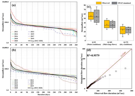
Figure 6.
The FDCs at GD (2012–2020): (a) the observed FDCs, (b) the simulated FDCs, (c) the comparison of the streamflow observed and simulated in Q 95, Q185, and Q275. In the boxplot, the interquartile ranges (IQR, i.e., 25th–75th quartiles) are represented by boxes, and whiskers extend to quartile 5 and quartile 95. (d) The scatter plot between the averages of observed and simulated FDA.
In Q10, the simulated results from 2016 to 2020 were smaller than the observed results (Figure 6a,b). The simulated Q10 from 2016 to 2020 was influenced by the average of the simulated runoff ratio of 38.5%. In particular, in 2020, the simulated Q10 was underestimated with a big difference of −255.7 m3/s compared to the observed Q10. The difference was caused by the summer flooding that occurred across the country in South Korea in 2020. In Q95, the simulated result was underestimated in 2015 when a drought occurred. It was overestimated in 2020 during a flood event. The average of simulated Q185 showed a slight difference of 0.5 m3/s compared to the average of observed Q185. For Q275, the simulated Q275 in 2015 was overestimated with a difference of +7.0 m3/s. The drought in 2015 affected model simulation. So, the model simulation did not reflect the trend of the observed data effectively. In the case of Q355, the average of the simulated results was bigger than the average of the observed results, with a difference of +3.9 m3/s. However, the simulated Q355 in 2020 was smaller than the observed Q355 with a difference of −11.8 m3/s. These results indicate that extreme values, such as Q10 or Q355, were not suitable for application as discharge boundary conditions in PHABSIM due to their high variability. The model did not effectively capture the observed data’s trends during droughts or floods. High flows can have significant impacts on instream conditions, including accelerated geomorphic changes in stream channels, and increased sedimentation, scour, and channelization. This combination can lead to a reduction in the quality and quantity of biotic habitats [41,42,43].
In Figure 6c, the black horizontal line indicates the median. The multiplication sign (×) means mean value. The observed and SWAT simulation results for 9 years in Q95, Q185, and Q275 were analyzed to be similar. In particular, the interquartile range (IQR) of Q185 and Q275 showed the same distributions for the streamflow. However, according to the SWAT simulated results (gray), the IQR was comparatively increased compared to what was observed (yellow) in Q95. In other words, the Q95 results from SWAT simulations show significant variation for 9 years.
The 9-year averages of the observed and simulated FDA results are compared one-to-one for the same durations to verify the relationship between the observed and simulated FDA (Figure 6d). The result shows an R2 value of 0.9579, indicating that the simulated streamflow closely followed the average trends of the observed streamflow during 2012–2020. However, for a streamflow over 200.0 m3/s, the SWAT simulation results show an underestimating tendency compared to the observed streamflow.
3.3. Results of Field Surveys for Selecting Dominant Fish Species and Constructing HSI
For estimating the optimal E-flow of fish species using PHABSIM, field surveys and the evaluation of HSI must be conducted [44]. In this study, the field surveys downstream of GD were conducted intensively during the dry season when the streamflow was the smallest throughout the year. These field surveys were conducted four times. Through these field surveys, the number of fish individuals sampled was 203 in 12 species of five families. Relative abundance (RA) was classified based on the number of fish observed, and dominant and subdominant species were identified. In addition, the distribution range by fish species was calculated by analyzing the depth and velocity data for each individual fish.
Table 4 shows the results of RA for the collected fish. The RA of Zacco platypus was assessed as 54.2% with a total 110 individuals and Cobitis hankugensis was assessed as 16.7%. The dominant species was Zacco platypus, which is widely distributed throughout the Nakdong River basin in the South Korea. The sub-dominant species were Cobitis hankugensis and Pseudogobio escocinus.
Table 4.
List and individual numbers of collected fish during survey period.
The dominant species was selected as the representative fish species, and the HSI for the representative fish species was calculated for water depth, velocity, and substrate. The representative methods of calculating the HSI are set out by the Washington Department of Fish and Wildlife (WDFW) [45] and Instream Flow and Aquatic Systems Group (IFASG) [15]. The WDFW method requires the number of fish observed in different depth and velocity sections within the fish survey area, as well as percentage data on the area occupied by each depth and velocity. The IFASG method determines the fitness based on the number of populations for each depth and the velocity of sections. The main difference between the two method is that the fitness of the WDFW method is determined based on the population density.
In this study, the HSI was calculated using the WDFW, which can effectively reflect the physical characteristics of rivers. The HSI is displayed as a graph by synthesizing the observation expectations and suitability index for each cross-section and survey period. An HSI of 1.0 provides an optimal physical habitat for target fish. The HSI of Zacco platypus was estimated at 0.4~0.6 m (depth), 0.3~0.5 m/s (velocity), and sand to fine gravel (substrate). Table 5 shows the range of HSI for Zacco platypus, and Figure 7 shows the HSI curves of depth and velocity with frequency of Zacco platypus observations. Despite the fish investigated being from the same river basin, the fish might differ in terms of their preferred habitat conditions in each stream because each stream has different physical characteristics. HIS is an important and sensitive factor when estimating the optimal E-flow, and it significantly influences the estimation of WUA. So, it is important to investigate in the specific stream that represents the physical habitat characteristics of the target fish. In this study, the HSI was constructed following field surveys, ensuring that our results effectively reflect the physical characteristics of the stream.
Table 5.
Results of optimal HSI range regarding depth, velocity, and substrate for Zacco platypus.
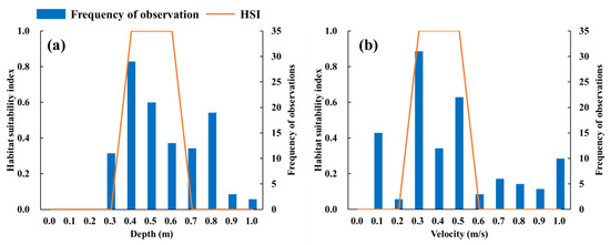
Figure 7.
HSI curves of depth and velocity for Zacco platypus (a) depth and (b) velocity.
3.4. PHABSIM Simulation and Estimation of E-Flow
In this study, the applicability of the SWAT model for providing PHABSIM input data was evaluated by simulating PHABSIM using the observed and SWAT-simulated streamflow and comparing the results of water surface elevation and velocity. For the PHABSIM discharge boundary condition, the averages of the observed Q185 (36.5 m3/s) and Q275 (23.8 m3/s) were applied to calibration discharges, and the averages of simulated Q185 (36.0 m3/s) and Q275 (23.8 m3/s) were applied to simulation discharges.
Table 6 shows the comparisons of water surface elevation and velocity when the observed and SWAT simulated discharge are respectively applied as boundary conditions of PHABSIM. As a result of the water surface elevation simulation, the water surface elevations of the observed Q185 and Q275 were 60.35 m and 60.11 m, respectively, and the SWAT-simulated discharges Q185 and Q275 were 60.23 m and 60.11 m, respectively. The SWAT-simulated results showed a tendency to underestimate compared to the observed results.
Table 6.
Comparisons of hydraulic factors between observed and SWAT-simulated discharges.
In the velocity simulation results, the velocities of the observed Q185 and Q275 were 0.53 m/s and 0.46 m/s, respectively, and the SWAT-simulated Q185 and Q275 were 0.50 m/s and 0.42 m/s, showing differences of −0.03 m/s and −0.04 m/s, respectively. The velocity was affected by the differences between the observed and SWAT-simulated discharges, as well as the input hydraulic data such as slope and roughness coefficient. Despite the error in the hydraulic model simulation, the water surface elevation and velocity were simulated effectively within an acceptable range.
PHABSIM calculates WUA and defines the flow that secures the largest WUA as the optimal E-flow. Figure 8 shows the WUA curve for Zacco platypus. Fish habitat area was generated with the area of 850.5 m2/1000 m from a discharge of 12.0 m3/s. This means that the average observed Q355 over 9 years satisfied the minimum flow duration required for the representative fish species of the target stream to survive, and that there was a large habitat area between the average observed Q355 and Q275. The optimal E-flow of the target stream was estimated at 20.0 m3/s, with an area of 110,058.8 m2/1000 m as the largest WUA, and the average WUA for the Zacco platypus was estimated at 31,905.3 m2/1000 m. When the WUA is at its maximum value, it means that the physical habitat conditions for the target fish species are the best. The optimal water velocity and depth of the target stream were evaluated at 20.0 m3/s.
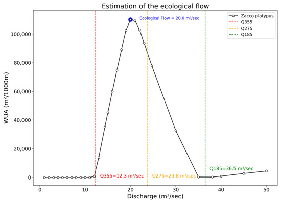
Figure 8.
The relationship of discharge and WUA with the average of observed FDA during 2012–2020 for Zacco platypus.
The ME manages IF for 114 spots across South Korea based on the River Act. They report on the amounts of IF, available IF, and future IF needed to be secured according to stream environmental criteria. These criteria include factors such as the average of Q355, water quality, salinity damage, landscapes, and ecology for each spot. There are 35 notification spots, including the JB spot, within the Nakdong River Basin. As mentioned earlier, E-flow is encompassed within the concept of IF. In South Korea, IF is designed to maintain the normal functions and state of rivers considering the various uses of river water for daily life, industry, agriculture, fishery, environmental improvement, and stream ecology. This indicates that the E-flow estimated by habitat modeling should be lower than the notified IF. In other words, it is important to compare the IF and E-flow, and to revise the errors between them by reviewing the E-flow result. The IF of JB downstream of PHABSIM modeling was reported to be 20.8 m3/s by ME. This means that the E-flow estimated by SWAT-PHABSIM coupled modeling was in an appropriate range compared to the notified IF, and that the modeling coupled with watershed and habitat models yielded effective simulations.
4. Discussion
E-flow is an essential component of future water management that must be considered when trying to maintain a healthy aquatic ecosystem. One of the challenging tasks that water management agencies face is how to extrapolate monitoring and field data to the watershed scale, especially in the context of water management planning. The presented SWAT and PHABSIM coupled modeling attempt provides insights into watershed-scale modeling for E-flow estimation. The evaluation of coupled modeling has demonstrated its ability to realistically depict the observed watershed and stream conditions. The coupled modeling successfully captured the major drivers relevant to estimating E-flow.
Our studies have confirmed previous research that coupled modeling approaches to for evaluate E-flow. Ref. [29] simulated model coupling between SWAT and PHABSIM to develop long-term discharge data in ungauged watersheds based on watershed characteristics and weather records. They suggested that the application of the integrated watershed–habitat model should confirm the accuracy of the predicted hydrologic curve used to estimate the WUA of the downstream habitat. They also found that the average relative error between the observed and simulated hydrographs was the smallest when the SWAT was simulated using a DEM with a 30 m by 30 m spatial resolution. Our study confirms these suggestions and supplements them based on the results of past research cases. The reasonable result regarding E-flow ensures the reliability of our study, indicating that the coupling of SWAT and PHABSIM is successful.
When linking two models with different scales, it is important to secure reliability through model calibration in the model that provides input data. We performed multi-points calibration at the two multi-purpose dams (ADD and IHD) and one streamflow gauging station (GD) using the observed dam inflows and streamflow data for the sake of improving the accuracy of the coupled modeling approach (Table 3 and Figure 5). The NSE at the three calibration points was 0.48 to 0.71. In particular, the result of the averaged NSE at the target stream (GD) was 0.48, which is not very high. The bed materials of GD mainly consisted of sand and fine gravel, which have good permeability (Table 1 and Table 5). Compared to the graphical results of the two multi-purpose dams (Figure 5), the recession curve of GD decreased steeply because the streamflow was rapidly discharged into the base flow. Also, the annual runoff ratio results of the observed and simulated streamflow were 37.1% and 35.9%, respectively, and these are determined by the R2 and NSE results. However, despite the relatively poor model efficiency, the average quantitative model calibration results of GD, such as the RMSE and PBIAS, were better than those of the two multi-purpose dams. Because the result of GD was directly used to determine the boundary conditions of PHABSIM, we focused on reducing the quantitative errors between the observed and simulated streamflow of GD.
A few models have used multivariate methods. CASiMiR (Computer Aided Simulation Model for Instream Flow Requirements) is a representative model that uses the multivariate method [46]. Refs. [47,48,49,50,51,52,53] used multivariate methods, such as fuzzy approaches. In general, aquatic ecosystem data can be expressed numerically through fuzzy rules based on expert opinions. Evaluations based on fuzzy approaches can reflect interactions between environmental factors and utilize experts’ opinions to develop physical habitat criteria [54]. Also, one of the most important advantages of the fuzzy approach is that it can better utilize inaccurate and inconsistent investigation results, as well as expert knowledge [48]. However, the fuzzy approach demands the selection and recruitment of experts, and the complexity increases with the number of experts involved. One of the most important disadvantages is that it relies entirely on the opinions and perspectives of experts, and fuzzy habitat simulation is thus not suitable for optimizing E-flow [51,52,55]. We found that the method is often used when there is insufficient data on the physical habitats of fish. Also, there have been many such cases in South Korea. Since we secured enough field data through field investigations, we used the univariate model. To derive an HSI more reflective of recent phenomenon, it should be selected based on monitoring data. Therefore, in the case of an HSI based on expert opinions, the experts’ subjective view is included, and there is a possibility that differences from the actual measurement data may be yielded through verification. Refs. [47,49] compared PHABSIM with other habitat simulation models, including River2D and CASiMiR, for urban and natural reach. The target reach here was longer than in our study. The main results show that E-flow estimated by the multivariate method was overestimated compared to other model univariate methods. These results indicate that PHABSIM is more suitable for estimating E-flow than other models, and the univariate method could effectively estimate the E-flow.
In South Korea, E-flow and IF are mainly managed during the dry season, rather than during the flood or normal seasons. Our results show that the IQR of the observed and simulated streamflow had smaller variabilities in Q185 and Q275 than in Q95. However, Q10 and Q355 were not particularly suitable for determining the boundary conditions of PHABSIM because the extreme values showed large variabilities between the observed and simulated streamflows (Figure 6c,d).
Our previous study estimated the optimal E-flow in the same target stream [56]. The overall watershed environmental conditions and modeling procedures were similar. The HSI for Zacco platypus was determined with referencing to a previous study in the Geum river basin, which is one of the five major rivers in South Korea. The HSI for Zacco platypus, as derived in the previous study, showed wider ranges of preferred water depth and velocity. The optimal E-flow estimated in the previous study was calculated as 20.0 m3/s, which is the same as in this study. However, the average WUA (76,817.0 m2/1000 m) and maximum WUA (111,904.5 m2/1000 m) in the previous study were much larger than in our study. Even if the HSI calculated at the different basins or streams is applied to the same fish species, the same E-flow may be calculated, but there will be a big difference in the estimated WUA, and the habitat area may be estimated inaccurately. The preferred habitat characteristics of fish are sensitive to hydrological alterations and differ according to seasonal and basin characteristics [57,58]. The hydrological alterations caused by seasonal changes can disrupt stream channel conditions and trigger chain reactions in fish habitats. These natural factors make it difficult to estimate the E-flow and WUA accurately. To estimate the E-flow and WUA accurately, it must be considered that a fish survey should be carried out in a season that represents the physical habitat characteristics of the fish, and the HSI should be appropriate.
The result of optimal E-flow derived through coupled modeling is included in the IF notified by ME (Figure 8). Because the IF notified by ME considers hydraulic facility operation and human activities, such as daily life, industry, agriculture, fishery, and environmental preservation, the estimated E-flow must be smaller than the notified IF. However, many studies do not consider this point, and only derive a quantitative E-flow result by modeling. To estimate the E-flow within an appropriate range, it must be compared with the IF notified upstream or downstream of the watershed.
We propose that SWAT-PHABSIM coupled modeling is suitable, given our results, and expect it will be useful for assessing the impacts of various watershed environmental change factors on aquatic ecosystems and E-flow in future study. Previous studies focused on coupled modeling between PHABSIM, and other models were focused on coupling with 2D models to visualize the habitat in aquatic ecosystems. While there are many studies focused on coupling with 2D models, there are few studies that focus on the changing watershed environments. While it is important to assess the current quality of habitats and estimate E-flow accordingly, it will also be important to evaluate future changes in terms of water management and ecosystems. Our study can make up for this defect and help in assessing past or future aquatic ecosystems by using various watershed environmental data. Many studies have predicted and assessed the impacts of watershed hydrology and water quality on environmental change using SWAT [59,60,61,62,63,64,65]. Also, [66] evaluated the aquatic ecosystem health index using stream water temperature and quality by applying the random forest technique. Furthermore, the SWAT development team has developed and provided the SWAT-WET tool, which can independently simulate the distribution or related characteristics of aquatic organisms in a lake or water body. Finally, these studies and characteristics of SWAT can be used as evidence that SWAT is a suitable tool for evaluating aquatic ecosystems and can be linked with PHABSIM.
5. Conclusions
This study performed coupled modeling, using watershed and physical habitat models SWAT and PHABSIM, and estimated the optimal E-flow for a target stream. To reflect the real basin and stream conditions and ensure the reliability of coupled modeling, we calibrated the SWAT using the observed hydrological data, considering two multi-purpose dams. For the calibration of SWAT, the average values of R2, NSE, RMSE, and PBIAS were 0.62, 0.57, 1.68 mm/day, and −16.6%, which are satisfactory. Through the FDA, we determined that the Q185 and Q275 were appropriate boundary conditions that could be applied to PHABSIM instead of the extreme flow duration components.
We selected as the representative fish species Zacco platypus, based on four field surveys of the target stream, and constructed the HSI via the WDFW method for this species in order to estimate the optimal E-flow. The optimal HSI ranges for Zacco platypus were evaluated as 0.4 to 0.6 m in depth, 0.3 to 0.5 m/s in velocity, and sand to fine gravel as regards the substrate. Using the average Q185 and Q275 values of SWAT and HSI, PHABSIM was simulated and estimated the optimal E-flow for the target stream. The optimal E-flow was estimated as 20.0 m3/s via coupled modeling, which is lower than that given by IF (21.0 m3/s), as notified by the government for the JB location. These results show that the applicability of coupled modeling using watershed and physical habitat models was high. Comparing the IF and estimated E-flow shows that the IF could be used as an effective tool to determine whether the E-flow has been estimated appropriately.
Overall, this study explains in detail the coupling process combing watershed and physical habitat models. However, aquatic ecosystems and habitats react to chemical characteristics such as water quality, as well as physical characteristics. Realistically, because aquatic ecosystem, E-flow, and habitat are closely related to chemical characteristics such as water quality, as well as physical characteristics, these should be considered in further studies, which will allow us to consider comprehensively the physiochemical characteristics and estimate an E-flow that appropriately reflects the chemical characteristics.
Author Contributions
Conceptualization, Y.-W.K. and S.-J.K.; formal analysis, J.-J.L. and J.-W.H.; investigation, J.-J.L. and J.-W.H.; methodology, J.-W.L. and S.-Y.W.; software, S.-Y.W.; supervision, S.-Y.W. and S.-J.K.; validation, J.-W.L.; writing—original draft preparation, Y.-W.K.; writing—review and editing, S.-Y.W. and S.-J.K. All authors have read and agreed to the published version of the manuscript.
Funding
This work was supported by the Korea Environment Industry & Technology Institute (KEITI) through the Aquatic Ecosystem Conservation Research Program, funded by the Korea Ministry of Environment (MOE) (2020003050001).
Data Availability Statement
The data used and analyzed during this study are available from the corresponding author on reasonable request.
Conflicts of Interest
The authors declare no conflict of interest.
References
- Park, J.S.; Jang, S.J.; Song, I.H. Estimation of an optimum ecological stream flow in the Banbyeon Stream using PHABSIM—Focused on Zacco platypus and Squalidus chankaensis tsuchigae. J. Korean Soc. Agric. Eng. 2020, 62, 51–62. [Google Scholar] [CrossRef]
- Prkash, S. Impact of climate change on aquatic ecosystem and its biodiversity: An overview. IJBI 2021, 3, 312–317. [Google Scholar] [CrossRef]
- Pan, B.; Yuan, J.; Zhang, X.; Wang, Z.; Chem, J.; Lu, J.; Yang, W.; Li, Z.; Zhao, N.; Xu, M. A review of ecological restoration technique in fluvial rivers. Int. J. Sediment Res. 2016, 31, 110–119. [Google Scholar] [CrossRef]
- Wang, Q.; Chen, J.; Qi, W.; Wang, D.; Lin, H.; Wu, X.; Wang, D.; Bai, Y.; Qu, J. Dam construction alters planktonic microbial predator-prey communities in the urban reaches of the Yangtze River. Water Res. 2023, 230, 119575. [Google Scholar] [CrossRef] [PubMed]
- Tharme, R.E. A global perspective on environmental flow assessment: Emerging trends in the development and application of environmental flow methodologies for rivers. River Res. Appl. 2003, 19, 397–441. [Google Scholar] [CrossRef]
- Jung, C.G.; Lee, J.W.; Ahn, S.R.; Hwang, S.J.; Kim, S.J. Assessment of ecological streamflow for maintaining good ecological water environment. J. Korean Soc. Agric. Eng. 2016, 58, 1–12. [Google Scholar] [CrossRef][Green Version]
- Woo, S.Y.; Kim, Y.W.; Kim, W.J.; Kim, S.H.; Kim, S.J. Development of water quality and aquatic ecosystem model for Andong Lake using SWAT-WET. J. Korea Water Resour. Assoc. 2021, 54, 719–730. [Google Scholar] [CrossRef]
- Hu, X.; Zuo, D.; Xu, Z.; Huamg, Z.; Liu, Z.; Han, Y.; Bi, Y. Response of macroinvertebrate community to water quality factors and aquatic ecosystem health assessment in a typical river in Beijing, China. Environ. Res. 2022, 212, 113474. [Google Scholar] [CrossRef]
- Greco, M.; Arbia, F.; Giampietro, R. Definition of ecological flow using IHA and IARI as an operative procedure for water management. Environments 2021, 8, 77. [Google Scholar] [CrossRef]
- Tennant, D.L. Instream flow regimes for fish, wildlife, recreation and related environmental resources. Fisheries 1976, 1, 6–10. [Google Scholar] [CrossRef]
- King, J.M.; Tharme, M.S.; De Viliers, M.S. Environmental Flow Assessments for Rivers: Manual for the Building Block Methodology; Water Research Commission: Pretoria, South Africa, 2008; pp. 1–364. [Google Scholar]
- Poff, N.L.; Zimmerman, J.K. Ecological responses to altered flow regimes: A literature review to inform the science and management of environmental flows. Freshw. Biol. 2010, 55, 194–205. [Google Scholar] [CrossRef]
- Verma, R.K.; Pandey, A.; Verma, S.; Mishra, S.K. A review of environmental flow assessment studies in India with implementation enabling factors and constraints. Ecohydrol. Hydrobiol. 2023; in press. [Google Scholar] [CrossRef]
- Leone, M.; Gentile, F.; Porto, A.L.; Ricci, G.F.; De Girolamo, A.M. Ecological flow in southern Europe: Status and trends in non-perennial rivers. J. Environ. Manag. 2023, 342, 118097. [Google Scholar] [CrossRef] [PubMed]
- Bovee, K.D. Development and Evaluation of Habitat Suitability Criteria for Use in the Instream Flow Incremental Methodology; National Ecology Center, Division of Wildlife and Contaminant Research, Fish and Wildlife Service: Washington, DC, USA, 1986.
- Bovee, K.D.; Lamb, B.L.; Bartholow, J.M.; Stalnaker, C.B.; Taylor, J. Stream Habitat Analysis Using the Instream Flow Incremental Methodology; US Geological Survey: Washington, DC, USA, 1998.
- Gore, J.A.; Crawford, D.J.; Addison, D.S. An analysis of artificial riffles and enhancement of benthic community diversity by physical habitat simulation (PHABSIM) and direct observation. River Res. Appl. 1998, 14, 69–77. [Google Scholar] [CrossRef]
- Kang, H.S.; Hur, J.W. Aquatic ecosystem and habitat improvement alternative in Hongcheon River using fish community. J. Korean Soc. Agric. Eng. 2012, 32, 331–343. [Google Scholar] [CrossRef][Green Version]
- Ministry of Environment. Notification of Instream FLOW Status; Ministry of Environment: Sejong, Republic of Korea, 2018.
- Jain, V.; Karnatak, N.; Raj, A.; Shekhar, S.; Bajracharya, B.; Jain, S. Hydrogeomorphic advancements in river science for water security in India. Water Secur. 2022, 16, 100118. [Google Scholar] [CrossRef]
- Mahapatra, S.; Jha, M.K. Environmental flow estimation for regulated rivers under data-scarce condition. J. Hydrol. 2022, 614, 128569. [Google Scholar] [CrossRef]
- Shinozaki, Y.; Shirakawa, N. A legislative framework for environmental flow implementation: 30-years operation in Japan. River Res. Appl. 2021, 37, 1323–1332. [Google Scholar] [CrossRef]
- Oueslati, O.; De Girolamo, A.M.; Abouabdilah, A.; Kjeldsen, T.R.; Lo Porto, A. Classifying the flow regimes of Mediterranean streams using multivariate analysis. Hydrol. Process. 2015, 29, 4666–4682. [Google Scholar] [CrossRef]
- D’Ambrosio, E.; De Girolamo, A.M.; Barca, E.; Ielpo, P.; Rulli, M. Characterising the hydrological regime of an ungauged temporary river system: A case study. Environ. Sci. Pollut. Res. 2017, 24, 13950–13966. [Google Scholar] [CrossRef]
- European Commission. Communication from the Commission to the European Parliament, the Council, the European Economic and Social Committee and the Committee of the Region. A Blueprint to Safeguard Europe’s Water Resource; European Commission: Brussels, Belgium, 2012. [Google Scholar]
- Leone, M.; Gentile, F.; Porto, A.L.; Ricci, G.F.; De Girolamo, A.M. Setting an ecological flow regime in a Mediterranean basin with limited data availability: The Locone River case study (S-E Italy). Ecohydrol. Hydrobiol. 2023, 23, 346–360. [Google Scholar] [CrossRef]
- Stefanidis, K.; Panagopoulos, Y.; Mimikou, M. Impact assessment of agricultural driven stressors on benthic macroinvertebrates using simulated data. Sci. Total Environ. 2016, 540, 32–42. [Google Scholar] [CrossRef] [PubMed]
- Piniewski, M.; Bieger, K.; Mehdi, B. Advancements in Soil and Water Assessment Tool (SWAT) for ecohydrological modelling and application. Ecohydrol. Hydrobiol. 2019, 19, 179–181. [Google Scholar] [CrossRef]
- Casper, A.F.; Dixon, B.; Earls, J.; Gore, J.A. Linking a spatially explicit watershed model (SWAT) with an in-stream fish habitat model (PHABSIM): A case study of setting minimum flows and levels in a low gradient, sub-tropical river. River Res. Appl. 2011, 27, 269–282. [Google Scholar] [CrossRef]
- Lee, J.Y.; Woo, S.Y.; Kim, Y.W.; Kim, S.J.; Pyo, J.C.; Cho, K.H. Dynamic calibration of phytoplankton blooms using the modified SWAT model. J. Clean Prod. 2022, 343, 131005. [Google Scholar] [CrossRef]
- Lee, J.W.; Lee, Y.G.; Woo, S.Y.; Kim, W.J.; Kim, S.J. Evaluation of water quality interaction by dam and weir operation using SWAT in the Nakdong River Basin of South Korea. Sustainability 2022, 12, 6845. [Google Scholar] [CrossRef]
- MOLIT Nakdong River Basic Plan Report; Ministry of Land Infrastructure and Transport: Sejong, Republic of Korea, 2009.
- Nash, J.E.; Sutcliffe, J.V. River forecasting using conceptual models: Part 1-a discussion of principles. J. Hydrol. 1970, 10, 280–290. [Google Scholar] [CrossRef]
- Gupta, H.V.; Sorooshian, S.; Yapo, P.O. Status of automatic calibration for hydrologic models: Comparison with multilevel expert calibration. J. Hydrol. Eng. 1999, 4, 135–143. [Google Scholar] [CrossRef]
- Singh, J.; Knapp, H.V.; Arnold, J.G.; Demissie, M. Hydrological modeling of the Iroquois river watershed using HSPF and SWAT. J. Am. Water Resour. Assoc. 2005, 41, 343–360. [Google Scholar] [CrossRef]
- Arnold, J.G.; Srinivasan, R.; Muttiah, R.S.; Williams, J.R. Large area hydrologic modeling assessment part I: Model development. J. Am. Water Resour. Assoc. 1998, 34, 73–89. [Google Scholar] [CrossRef]
- Arnold, J.G.; Moriasi, D.N.; Gassman, P.W.; Abbaspour, K.C.; White, M.J.; Srinivasan, R.; Santhi, C.; Harmel, R.D.; van Griensven, A.; Van Liew, M.W.; et al. SWAT: Model use, calibration, and validation. Trans. ASABE 2012, 55, 1491–1508. [Google Scholar] [CrossRef]
- Neitsch, S.L.; Arnold, J.G.; Kiniry, J.R.; Williams, J.R.; King, K.W. Soil and Water Assessment Tool Theoretical Documentation: Version 2009; Texas Water Resources Institute: College Station, TX, USA, 2009. [Google Scholar]
- Waddle, T. PHABSIM for Windows User’s Manual and Exercises; US Geological Survey: Washington, DC, USA, 2011.
- Stalnaker, C.B.; Lamb, B.L.; Henriksen, J.; Bovee, K.; Bartholow, J. The Instream Flow Incremental Methodology: A Primer for IFIM; Biological Report 29; US Department of the Interior, National Biological Service: Washington, DC, USA, 1995.
- Wolman, M.G. A cycle of erosion and sedimentation in urban river channels. Geogr. Ann. Ser. A Phys. Geogr. 1967, 49, 385–395. [Google Scholar] [CrossRef]
- Hammer, T.R. Stream channel enlargement due to urbanization. Water Resour. Res. 1972, 8, 1530–1540. [Google Scholar] [CrossRef]
- Bledsoe, B.; Watson, C. Effects of urbanization on channel instability. J. Am. Water Resour. Assoc. 2001, 37, 255–270. [Google Scholar] [CrossRef]
- Kim, S.H.; Jung, K.J.; Kang, H.S. Response of fish community to building block methodology mimicking natural flow regime patterns in Nakdong River in South Korea. Sustainability 2022, 14, 3587. [Google Scholar] [CrossRef]
- Washington Department of Fish and Wildfire (WDFW). Comprehensive Management Plan for Puget Sound Chinook: Harvest Management Component; Northwest Indian Fisheries Commission: Olympia, Greece; Washington, DC, USA, 2004.
- Schneider, M.; Noack, M.; Gebler, T.; Kpecki, L. Handbook for the Habitat Simulation Model CASiMiR; Schneider & Jorde Ecological Engineering GmbH and University of Stuttgart Institute of Hydraulic Engineering: Stuttgart, Germany, 2010. [Google Scholar]
- Jung, S.H.; Jang, J.Y.; Choi, S.U. Physical habitat modeling in Dalcheon stream using fuzzy logic. J. Korea Water Resour. Assoc. 2012, 45, 229–242. [Google Scholar] [CrossRef]
- Zhang, H.; Sun, T.; Shao, D.; Yang, W. Fuzzy logic method for evaluating habitat suitability in an Estuary affected by land reclamation. Wetlands 2014, 36, 19–30. [Google Scholar] [CrossRef]
- Jang, K.H.; Park, Y.K.; Kim, K.O.; Chung, M. A comparative study on assessment model of ecological flow rate considering instream flow incremental methodology. J. KSET 2017, 18, 604–616. [Google Scholar] [CrossRef]
- Yi, Y.; Cheng, X.; Yang, Z.; Wieprecht, S.; Zhang, S.; Wu, Y. Evaluating the ecological influence of hydraulic project: A review of aquatic habitat suitability models. Renew. Sust. Energ. Rev. 2017, 68, 748–762. [Google Scholar] [CrossRef]
- Sedighkia, M.; Abdoli, A.; Datta, B. Optimizing monthly ecological flow regime by a coupled fuzzy physical habitat simulation-genetic algorithm method, Environ. Syst. Decis. 2021, 41, 425–436. [Google Scholar] [CrossRef]
- Ouellet, V.; Mocq, J.; El Adlouni, S.E.; Krause, S. Improve performance and robustness of knowledge-based fuzzy logic habitat models. Environ. Modell. Softw. 2021, 144, 105138. [Google Scholar] [CrossRef]
- Wang, X.; Deng, Y.; An, R.; Yan, Z.; Yang, Y.; Tuo, Y. Evaluating the impact of power station regulation on the suitability of drifting spawning fish habitat based on the fuzzy evaluation method. Sci. Total Environ. 2023, 866, 161327. [Google Scholar] [CrossRef] [PubMed]
- Mouton, M.A.; Schneider, M.; Depestele, J.; Goethals, P.L.M.; De Pauw, N. Fish habitat modelling as a tool for river management. Ecol. Eng. 2007, 29, 305–315. [Google Scholar] [CrossRef]
- Lu, Y.; Chen, Y.S. A review of river habitat assessments and applications. Acta Hydrobiol. Sin. 2020, 44, 670–684. [Google Scholar] [CrossRef]
- Kim, Y.W.; Byeon, S.D.; Park, J.S.; Woo, S.Y.; Kim, S.J. Evaluation of applicability of linkage modeling using PHABIM and SWAT. J. Korea Water Resour. Assoc. 2021, 54, 819–833. [Google Scholar] [CrossRef]
- Wolter, C.; Bischoff, A. Seasonal changes of fish diversity in the main channel of the large lowland River Oder. River Res. Appl. 2021, 17, 595–608. [Google Scholar] [CrossRef]
- Helms, B.S.; Schoonover, J.E.; Feminella, J.W. Assessing influences of hydrology, physicochemistry, and habitat on stream fish assemblages across a changing landscape. J. Am. Water Resour. Assoc. 2009, 45, 157–169. [Google Scholar] [CrossRef]
- Kim, I.K.; Arnhold, S.; Ahn, S.R.; Le, Q.B.; Kim, S.J.; Park, S.J.; Koellner, T. Land use change and ecosystem services in mountainous watersheds: Predicting the consequences of environmental policies with cellular automata and hydrological modeling. Environ. Modell. Softw. 2019, 122, 103982. [Google Scholar] [CrossRef]
- Ahn, S.R.; Kim, S.J. Assessment of watershed health, vulnerability, and resilience for determining protection and restoration priorities. Environ. Modell. Softw. 2019, 122, 103926. [Google Scholar] [CrossRef]
- Kim, H.J.; Cho, K.; Kim, Y.; Park, H.; Lee, J.W.; Kim, S.J.; Chae, Y. Spatial assessment of water-use vulnerability under future climate and socioeconomic scenarios within a River Basin. J. Water Resour. Plan. Manage.-ASCE. 2020, 146, 05020011. [Google Scholar] [CrossRef]
- Woo, S.Y.; Kim, S.J.; Lee, J.W.; Kim, S.H.; Kim, Y.W. Evaluating the impact of inter-basin water transfer on water quality in the recipient river basin with. Sci. Total Environ. 2021, 776, 05020011. [Google Scholar] [CrossRef] [PubMed]
- Feng, M.; Shen, Z. Assessment of the impacts of land use change on non-point source loading under future climate scenario using the SWAT model. Water 2021, 13, 874. [Google Scholar] [CrossRef]
- Abuhay, W.; Gashaw, T.; Tsegaye, W. Assessing impacts of land use/land cover changes on the hydrology of Upper Gilgel Abbay watershed using the SWAT model. J. Agric. Food Res. 2023, 12, 100535. [Google Scholar] [CrossRef]
- Uniyal, B.; Kosatica, E.; Koellner, T. Spatial and temporal variability of climate change impacts on ecosystem services in small agricultural catchments using the Soil and Water Assessment Tool (SWAT). Sci. Total Environ. 2023, 875, 162520. [Google Scholar] [CrossRef] [PubMed]
- Woo, S.Y.; Chung, G.J.; Lee, J.W.; Kim, S.J. Evaluation of watershed scale aquatic ecosystem health by SWAT modeling and random forest technique. Sustainability 2019, 11, 3397. [Google Scholar] [CrossRef]


Disclaimer/Publisher’s Note: The statements, opinions and data contained in all publications are solely those of the individual author(s) and contributor(s) and not of MDPI and/or the editor(s). MDPI and/or the editor(s) disclaim responsibility for any injury to people or property resulting from any ideas, methods, instructions or products referred to in the content. |
© 2023 by the authors. Licensee MDPI, Basel, Switzerland. This article is an open access article distributed under the terms and conditions of the Creative Commons Attribution (CC BY) license (https://creativecommons.org/licenses/by/4.0/).