
A Mathematical Method for Estimating the Critical Slope Angle of Sheet Erosion

Abstract
:1. Introduction
2. Data and Methods
2.1. Basic Formulas
2.2. Mathematical Equation Derivations
2.2.1. Derivation of Instantaneous CSA Estimation Equation
2.2.2. Derivation of Cumulative CSA Estimation Equation
2.3. Validation of Mathematical Equation Method
2.3.1. Validation by Field Observations
2.3.2. Validation by Water Erosion Prediction Project (WEPP) Model Simulations
2.4. Validation of Mathematical Equation Method
3. Results and Discussion
3.1. Validation of Mathematical Equations
3.1.1. Comparison to Field Plot Observations
3.1.2. Comparison to WEPP Simulation Results
3.2. Characteristics of Instantaneous and Cumulative CSAs
3.2.1. Modeling the Change in Instantaneous CSA
3.2.2. Modeling the Change in Cumulative CSA
3.2.3. Modeling Instantaneous CSA and Cumulative CSA in Different Rainfall Conditions
3.3. Effect of Manning Coefficient (n) on the CSA
3.4. Improvements of the Mathematical Equations
3.5. Limitations
4. Conclusions
Author Contributions
Funding
Data Availability Statement
Acknowledgments
Conflicts of Interest
Notation
| τ | shear stress of overland flow |
| ρ | density of overland flow |
| g | acceleration of gravity |
| n | Manning coefficient |
| I | rainfall intensity |
| f | soil infiltration rate |
| L | incline length of slope |
| α | slope angle |
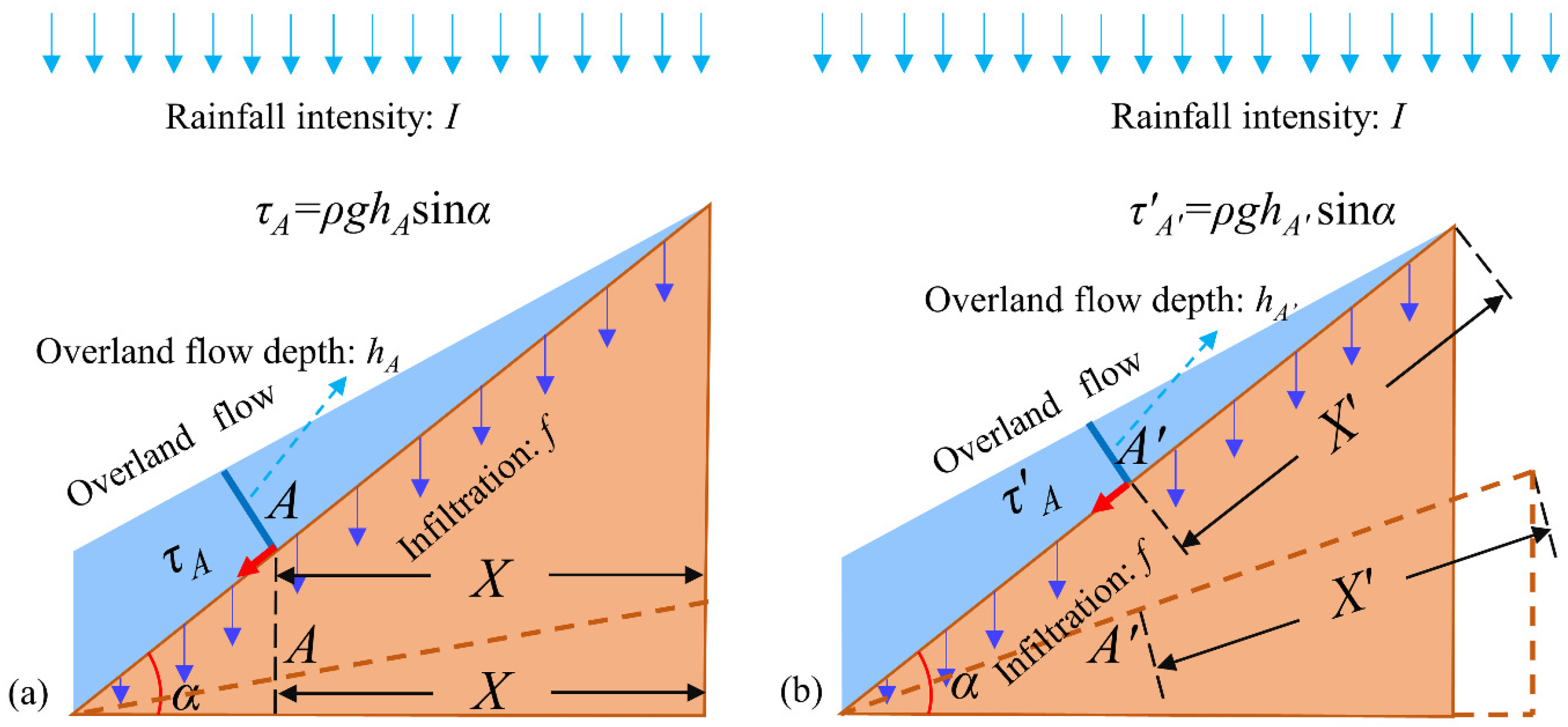
| τA | shear stress at point A (Figure 1a) |
| τ′A | shear stress at point A′ (Figure 1b) |
| X | horizontal projective length from A to the top of the slope (Figure 1a) |
| X′ | incline length from A′ point to the top of the slope (Figure 1b) |
| TA | cumulative shear stress at point A during rainfall (Figure 1a) |
| T′A | cumulative shear stress at point A′ during rainfall (Figure 1b) |
| I(t) | change in rainfall intensity with time during rainfall |
| f(t) | change in soil infiltration rate with time during rainfall |
| t1 | time of overland flow initiation |
| t2 | time of overland flow cessation. |
| N0 | friction coefficient (nondimensional) |
| d | grain size of soil (mm) |
| rs | soil dry bulk density (N m−3) |
| r | water density (N m−3) |
| k | effective saturated hydraulic conductivity (mm min−1) |
| M | effective porosity |
| S | wetting front soil suction head (m) |
| hp | cumulative infiltration depth (mm) |
| kt | transport coefficient (WEPP model) |
| τc | adjusted soil critical shear stress (WEPP model) |
| fmean | mean of effective soil hydraulic conductivity ((mm h−1)) |
Appendix A
Appendix A.1. Derivation of the Shear Force Equation for Overland Flow

References
- Mandal, D.; Giri, N.; Srivastava, P. The magnitude of erosion-induced carbon (C) flux and C-sequestration potential of eroded lands in India. Eur. J. Soil Sci. 2020, 71, 151–168. [Google Scholar] [CrossRef]
- Pimentel, D. Soil erosion: A food and environmental threat. Environ. Dev. Sustain. 2006, 8, 119–137. [Google Scholar] [CrossRef]
- von Ruette, J.; Lehmann, P.; Or, D. Effects of rainfall spatial variability and intermittency on shallow landslide triggering patterns at a catchment scale. Water Resour. Res. 2014, 50, 7780–7799. [Google Scholar] [CrossRef]
- Borrelli, P.; Robinson, D.A.; Fleischer, L.R.; Lugato, E.; Ballabio, C.; Alewell, C.; Meusburger, K.; Modugno, S.; Schuett, B.; Ferro, V.; et al. An assessment of the global impact of 21st century land use change on soil erosion. Nat. Commun. 2017, 8, 2013. [Google Scholar] [CrossRef] [PubMed]
- Montgomery, D.R. Soil erosion and agricultural sustainability. Proc. Natl. Acad. Sci. USA 2007, 104, 13268–13272. [Google Scholar] [CrossRef]
- Huang, C.H. Empirical analysis of slope and runoff for sediment delivery from interrill areas. Soil Sci. Soc. Am. J. 1996, 60, 1279–1280. [Google Scholar] [CrossRef]
- Parsons, A.J. How reliable are our methods for estimating soil erosion by water? Sci. Total Environ. 2019, 676, 215–221. [Google Scholar] [CrossRef]
- Zhang, Q.W.; Wang, Z.L.; Wu, B.; Shen, N.; Liu, J.E. Identifying sediment transport capacity of raindrop-impacted overland flow within transport-limited system of interrill erosion processes on steep loess hillslopes of China. Soil Tillage Res. 2018, 184, 109–117. [Google Scholar] [CrossRef]
- Jouquet, P.; Janeau, J.L.; Pisano, A.; Hai Tran, S.; Orange, D.; Luu Thi Nguyet, M.; Valentin, C. Influence of earthworms and termites on runoff and erosion in a tropical steep slope fallow in Vietnam: A rainfall simulation experiment. Appl. Soil Ecol. 2012, 61, 161–168. [Google Scholar] [CrossRef]
- Zhang, X.; Yu, G.Q.; Li, Z.B.; Li, P. Experimental study on slope runoff, erosion and sediment under different vegetation types. Water Resour. Manag. 2014, 28, 2415–2433. [Google Scholar] [CrossRef]
- Wang, H.; Zhang, G.H. Temporal variation in soil erodibility indices for five typical land use types on the Loess Plateau of China. Geoderma 2021, 381, 114695. [Google Scholar] [CrossRef]
- Cheng, Q.J.; Ma, W.J.; Cai, Q.G. The relative importance of soil crust and slope angle in runoff and soil loss: A case study in the hilly areas of the Loess Plateau, North China. GeoJournal 2008, 71, 117–125. [Google Scholar] [CrossRef]
- Wu, S.B.; Yu, M.H.; Chen, L. Nonmonotonic and spatial-temporal dynamic slope effects on soil erosion during rainfall-runoff processes. Water Resour. Res. 2017, 53, 1369–1389. [Google Scholar] [CrossRef]
- Horton, R.E. Erosional development of streams and their drainage basins-hydro physical approach to quantitative morphology. Geol. Soc. Am. Bull. 1945, 56, 275–370. [Google Scholar] [CrossRef]
- Liu, Q.Q.; Chen, L.; Li, J.C. Influences of slope gradient on soil erosion. Appl. Math. Mech. 2001, 22, 510–519. [Google Scholar] [CrossRef]
- Giménez, R.; Govers, G. Flow detachment by concentrated flow on smooth and irregular beds. Soil Sci. Soc. Am. J. 2002, 66, 1475–1483. [Google Scholar] [CrossRef]
- Govers, G.; Giménez, R.; Govers, R.; Van Oost, K. Rill erosion: Exploring the relationship between experiments, modelling and field observations. Earth-Sci. Rev. 2007, 84, 87–102. [Google Scholar] [CrossRef]
- Liu, G.; Zheng, F.L.; Wilson, G.V.; Xu, X.M.; Liu, C. Three decades of ephemeral gully erosion studies. Soil Tillage Res. 2021, 212, 105046. [Google Scholar] [CrossRef]
- Liao, Y.S.; Cai, Q.G.; Cheng, Q.J. Critical topographic condition for slope erosion in hilly-gully region of Loess Plateau. Soil Water Conserv. 2008, 2, 32–38. [Google Scholar] [CrossRef]
- Chen, X.A.; Cai, Q.G.; Zhang, L.C.; Qi, J.Y.; Zheng, M.G.; Nie, B.B. Research on critical slope of soil erosion in a Hilly Loess Region on the Loess Plateau. J. Mt. Sci. 2010, 28, 415–421. [Google Scholar] [CrossRef]
- Foster, R.L.; Martin, G.L. Effect of unit weight and slope on erosion. J. Irrig. Drain. Eng. 1969, 95, 551–561. [Google Scholar] [CrossRef]
- He, J.J.; Cai, G.Q.; Liu, S.B. Effects of slope gradient on slope runoff and sediment yield under different single rainfall conditions. J. Appl. Ecol. 2012, 23, 1263–1268. [Google Scholar] [CrossRef]
- Fu, S.H.; Liu, B.Y.; Liu, H.P.; Xu, L. The effect of slope on interrill erosion at short slopes. Catena 2011, 84, 29–34. [Google Scholar] [CrossRef]
- Liu, Q.Q.; Xiang, H.; Singh, V.P. A simulation model for unified interrill erosion and rill erosion on hillslopes. Hydrol. Process. 2006, 20, 469–486. [Google Scholar] [CrossRef]
- Chen, Y.Z. A preliminary analysis of the processes of sediment yield in small catchment on the Loess Plateau. Geogr. Res. 1983, 2, 35–47. [Google Scholar] [CrossRef]
- Zhu, P.; Zhang, G.; Wang, H.; Xing, S. Soil infiltration properties affected by typical plant communities on steep gully slopes on the Loess Plateau of China. J. Hydrol. 2020, 590, 125535. [Google Scholar] [CrossRef]
- Flanagan, D.; Nearing, M. USDA-Water Erosion Prediction Project: Hillslope Profile and Watershed Model Documentation; NSERL Report No. 10; National Soil Erosion Research Laboratory, USDA-Agricultural Research Service: West Lafayette, IN, USA, 1995.
- Cochrane, T.A.; Flanagan, D.C. Representative hillslope methods for applying the WEPP model with DEMS and GIS. Trans. ASAE 2003, 46, 1041–1049. [Google Scholar] [CrossRef]
- Abaci, O.; Papanicolaou, A.N.T. Long-term effects of management practices on water-driven soil erosion in an intense agricultural sub-watershed: Monitoring and modelling. Hydrol. Process. 2009, 23, 2818–2837. [Google Scholar] [CrossRef]
- Chen, L.; Young, M.H. Green-Ampt infiltration model for sloping surfaces. Water Resour. Res. 2006, 42, W07420. [Google Scholar] [CrossRef]
- Green, W.H.; Ampt, G.A. Studies on soil physics. J. Agric. Sci. 1911, 4, 1–24. [Google Scholar] [CrossRef]
- Ascough, J.C.; Baffaut, C.; Nearing, M.A.; Liu, B.Y. The WEPP watershed model: I. Hydrology and erosion. Trans. ASAE 1997, 40, 921–933. [Google Scholar] [CrossRef]
- Alaoui, A.; Helbling, A. Evaluation of soil compaction using hydrodynamic water content variation: Comparison between compacted and non-compacted soil. Geoderma 2006, 134, 97–108. [Google Scholar] [CrossRef]
- Fullen, M. Compaction, hydrological processes and soil erosion on loamy sands in east Shropshire, England. Soil Tillage Res. 1985, 6, 17–29. [Google Scholar] [CrossRef]
- Yu, M.; Zhang, L.; Xu, X.; Feger, K.-H.; Wang, Y.; Liu, W.; Schwärzel, K. Impact of land-use changes on soil hydraulic properties of Calcaric Regosols on the Loess Plateau, NW China. J. Soil Sci. Plant. Nut. 2015, 178, 486–498. [Google Scholar] [CrossRef]
- Chen, L.; Sela, S.; Svoray, T.; Assouline, S. Scale dependence of Hortonian rainfall-runoff processes in a semiarid environment. Water Resour. Res. 2016, 52, 5149–5166. [Google Scholar] [CrossRef]
- Cui, Z.; Wu, G.L.; Huang, Z.; Liu, Y. Fine roots determine soil infiltration potential than soil water content in semiarid grassland soils. J. Hydrol. 2019, 578, 124023. [Google Scholar] [CrossRef]
- Zhang, G.H.; Luo, R.T.; Cao, Y.; Shen, R.C.; Zhang, X.C. Impacts of sediment load on Manning coefficient in supercritical shallow flow on steep slopes. Hydrol. Process. 2010, 24, 3909–3914. [Google Scholar] [CrossRef]
- Vastila, K.; Jarvela, J. Characterizing natural riparian vegetation for modeling of flow and suspended sediment transport. J. Soil. Sediment. 2018, 18, 3114–3130. [Google Scholar] [CrossRef]
- Shen, E.; Liu, G.; Dan, C.; Chen, X.; Ye, S.; Li, R.; Li, H.; Zhang, Q.; Zhang, Y.; Guo, Z. Estimating Manning’s coefficient n for sheet flow during rainstorms. Catena 2023, 226, 107093. [Google Scholar] [CrossRef]
- Ding, W.F.; Li, Y.L.; Wang, Y.F.; Cheng, D.B.; Zhang, P.C.J. Study on runoff hydrodynamics of purple soil slope under the rainfall simulation experiment. Soil Water Conserv. 2010, 24, 66–69. [Google Scholar] [CrossRef]
- Giménez, R.; Govers, G. Interaction between bed roughness and flowhydraulics in eroding rills. Water Resour. Res. 2001, 37, 791–799. [Google Scholar] [CrossRef]
- Zhao, L.; Liang, X.; Wu, F. Soil surface roughness change and its effect on runoff and erosion on the Loess Plateau of China. J. Arid Land 2014, 6, 400–409. [Google Scholar] [CrossRef]
- Zheng, Z.C.; He, S.Q.; Wu, F.Q. Changes of soil surface roughness under water erosion process. Hydrol. Process. 2014, 28, 3919–3929. [Google Scholar] [CrossRef]
- Bahddou, S.; Otten, W.; Whalley, W.R.; Shin, H.C.; El Gharous, M.; Rickson, R.J. Changes in soil surface properties under simulated rainfall and the effect of surface roughness on runoff, infiltration and soil loss. Geoderma 2023, 431, 116341. [Google Scholar] [CrossRef]
- Fu, S.; Mu, H.; Liu, B.; Yu, X.; Liu, Y. Effect of plant basal cover on velocity of shallow overland flow. J. Hydrol. 2019, 577. [Google Scholar] [CrossRef]
- Fox, D.M.; Bryan, R.B. The relationship of soil loss by interrill erosion to slope gradient. Catena 2000, 38, 211–222. [Google Scholar] [CrossRef]
- Wang, C.F.; Wang, B.; Wang, Y.Q.; Wang, Y.J.; Zhang, W.L.; Yan, Y.K. Impact of near-surface hydraulic gradient on the interrill erosion process. Eur. J. Soil Sci. 2020, 71, 598–614. [Google Scholar] [CrossRef]
- Gabet, E.J.; Dunne, T. A stochastic sediment delivery model for a steep Mediterranean landscape. Water Resour. Res. 2003, 39, 1237. [Google Scholar] [CrossRef]
- Woolhiser, D.A.; Liggett, A. Unsteady, one-dimensional flow over a plane—The rising hydrograph. Water Resour. Res. 1967, 3, 753–771. [Google Scholar] [CrossRef]


| Parameter | Value | Parameter | Value |
|---|---|---|---|
| I (I10, mm min−1) | 7.5, 8.9, 7.9, 10.9, 8.2, 8.2 | rs(N m−3) | 1300 |
| f, k (mm min−1) | 0.625 | r (N m−3) | 1100 |
| d (mm) | 0.05 | L (m) | 20 |
| N0 | 0.047 | n | 0.03 |
| M | 0.45 | S (mm) | 60 |
| Parameter | Value | Parameter | Value |
|---|---|---|---|
| I (mm h−1) | 45 | Kt (m0.5 s2 kg−0.5) | 0.029 |
| fmean (mm h−1) | 22.5 | τc (Pa) | 0.025 |
| SM (m) | 0.0173 | Slope length (m) | 22.1 |
Disclaimer/Publisher’s Note: The statements, opinions and data contained in all publications are solely those of the individual author(s) and contributor(s) and not of MDPI and/or the editor(s). MDPI and/or the editor(s) disclaim responsibility for any injury to people or property resulting from any ideas, methods, instructions or products referred to in the content. |
© 2023 by the authors. Licensee MDPI, Basel, Switzerland. This article is an open access article distributed under the terms and conditions of the Creative Commons Attribution (CC BY) license (https://creativecommons.org/licenses/by/4.0/).
Share and Cite
Wang, M.; Chen, D.; Wang, Y.; Pan, Z.; Pan, Y. A Mathematical Method for Estimating the Critical Slope Angle of Sheet Erosion. Water 2023, 15, 3341. https://doi.org/10.3390/w15193341
Wang M, Chen D, Wang Y, Pan Z, Pan Y. A Mathematical Method for Estimating the Critical Slope Angle of Sheet Erosion. Water. 2023; 15(19):3341. https://doi.org/10.3390/w15193341
Chicago/Turabian StyleWang, Mingfeng, Dingjiang Chen, Yucang Wang, Zheqi Pan, and Yi Pan. 2023. "A Mathematical Method for Estimating the Critical Slope Angle of Sheet Erosion" Water 15, no. 19: 3341. https://doi.org/10.3390/w15193341