Evaluation of Various Turbulence Models and Large Eddy Simulation for Stall Prediction in a Centrifugal Pump

Abstract

Rotational stall is an unstable flow phenomenon that reduces the performance of centrifugal pumps, usually occurring under partial load conditions. It causes instability in the flow resulting in intense vibrations and noise under certain flow conditions. In this study, the one-equation Wray–Agarwal (WA) turbulence model, which was recently developed, is employed to numerically simulate the internal flow field of a centrifugal pump under the deep stall condition. The aim of this study is to examine the prediction accuracy for stall by using the WA turbulence model. The method based on computational fluid dynamics (CFD) has been widely applied for investigation of complex flow patterns in pumps by solving Reynolds-averaged Navier-Stokes (RANS) equations. Particle image velocimetry (PIV) experimental results were compared with simulations predicted using the WA, renormalization group (RNG) k−ε, shear stress transport (SST) k−ω, and realizable k−ε turbulence models and large eddy simulations (LES). The comparisons indicated that the WA turbulence model can accurately predict the flow separation and has a good agreement with the PIV data. The WA model adds a cross-diffusion term and a blending function to the eddy viscosity R equation, so that this model could be expressed as a one-equation k−ω model or one-equation k−ε model as needed by using the switching function. The results show the strong potential of the WA model for accurately computing the stall in rotating fluid machinery. The outcomes of the study are useful in development and optimization of fluid machinery with a low calculation cost and a high accuracy.

1. Introduction

Centrifugal pumps are among the most commonly used and important general mechanical equipment. When centrifugal pumps are operated at low flow conditions with deviation from the design point, stall is likely to occur due to changes in the inlet angle of attack. Firstly, the flow separation occurs and develops around the suction surface of the impeller blades. Then, the separation vortex blocks the channel and forms a stall cell under deep stall conditions [1,2]. The stall phenomenon in centrifugal pumps can be divided into rotating stall and alternative stall. Rotating stall often occurs with an odd number of blades, where the stall cell propagates in the opposite direction to the impellers’ rotation [3]. The alternative stall often occurs with an even number of blades. The alternative stall refers to the alternating distribution of stall cells in the impeller passages. The circumferential propagation velocity of the stall cell is zero, which is periodically symmetrical [4,5]. When stalling occurs in a centrifugal pump, the stall cells destroy the flow field structure with resulting humps and positive slopes in the pump performance curve. It also leads to additional dynamic load on the blades. Under some flow conditions it may cause vibration, fatigue and even fracture of the blades [6,7,8]. In addition to reducing the efficiency of the pump, the stall phenomenon also has a serious negative influence on the safety and stability of the pump system [9,10]. At present, the research on centrifugal pump stall is still very limited, and therefore in-depth research considering all aspects is needed to explore the mechanism of stall and use this understanding to improve the efficiency and reliability of centrifugal pumps.

Computational fluid dynamics (CFD) is one of the most widely used methods in the design and optimization of fluid machinery [11,12]. The advantage of CFD is that it can visualize internal flow fields such as velocity and pressure. It is also useful to optimize the geometry parameters to enhance the hydraulic performance of fluid machinery [13]. Turbulence models play an important role in achieving accurate and efficient simulation results using RANS equations. The direct numerical simulation (DNS) method employs the transient Navier-Stokes equations to solve the turbulent flow and in principle can provide very accurate results [14]. However, DNS requires very small spatial grids and step sizes to resolve the detailed spatial structure and temporal properties of turbulent flow, which can be very computationally intensive and may not be feasible on the currently available computing hardware [15] for the flow conditions in fluid machinery. The flow in fluid machinery is turbulent with high Reynolds numbers, where large scale vortex structures play the leading role and small-scale vortex structures play the role of transmission and dissipation of energy. Based on this idea, Smagorinsky proposed the large eddy simulation (LES) method in 1963. The fundamental principle of LES is to filter the small-scale eddy structures through a filtering function and then directly calculate the large-scale eddy structures and their effects on the turbulent flow solution; the other small-scale eddies are modeled using a sub–grid–scale Smagorinsky model [16]. LES is less computationally intensive compared to DNS but still requires a higher near-wall mesh density than the RANS solutions and therefore more computing resources. Until now, RANS is the most commonly used method for the numerical simulation of fluid machinery [17,18].

RANS equations do not solve the instantaneous Navie-r-Stokes equations directly, but average the transient fluctuations and employ a turbulence model to model the turbulent stresses and then solve the simpler time-averaged equations [18]. In the past five decades, various RANS turbulence models have been developed. The difference among these turbulence models lies in the mathematical modeling of Reynolds stresses employing different assumptions [19]. Depending on the number of partial differential equations used to calculate the eddy viscosity, turbulence models are usually classified as zero-, one- and two-equation models [20,21]. At present, the two-equation turbulence models are the most widely used for prediction of flow field characteristics of pumps under design flow conditions [22]. However, when the flow deviates from the design flow condition, the vortex viscosity assumption will distort the calculated average flow due to the separated flow and the influence of vortex flow. The simulation results of different models under off-design conditions are different [23]. Furthermore, the prediction of complex 3D flow needs a large number of grids to solve the RANS equations, which requires larger computational resources. Therefore, it is important to use fewer transport equations to develop more accurate and efficient turbulence models [24]. One-equation turbulence models are used to calculate eddy viscosity directly via solving the transport equation for eddy viscosity rather than having to calculate two or more turbulence variables. One-equation turbulence models are simpler and require less computational time compared with two-equation turbulence models. However, various existing one-equation turbulence models have low accuracy in predicting non-equilibrium flows [25]. Therefore, it is important to improve the prediction accuracy of one-equation turbulence models for a better understanding of turbulence.

The recently developed Wray-Agarwal (WA) turbulence model is a one-equation model based on k−ω closure [26] and shows great potential in predicting complex three-dimensional (3D) flows [27,28,29]. The WA model showed higher accuracy than the Spalart-Allmaras (SA) model for many flows, and can accurately simulate non-equilibrium and low Reynolds number effects in the near-wall region. Han et al. [30] used the WA model and four other commonly used one- or two-equation turbulence models to predict the internal flow of a three-dimensional U-bend. The results showed that the velocity iso-surface calculated using the WA model is largely consistent with the test results. Ouyang et al. [31] employed the WA model to calculate the multiphase flow in a rotating packed bed. Their results showed that the WA model is superior to the other two-equation models in predicting free shear flow. Ji et al. [24] used the WA turbulence model for a centrifugal pump with semi-spiral suction chambers, the results showed that this model could calculate the energy performance of centrifugal pumps effectively in the entire operating range, and had higher accuracy than other models. In over 70 applications to date, the WA model has shown its ability to predict complex 3D flows quite accurately and, in many instances, exhibited superior performance compared to SA and other two-equation models based on k−ε closure.

The operation of centrifugal pumps deviates from the design conditions, resulting in a very complex internal flow field, which has high requirements on the efficacy of a turbulence model. Pederson [32] used LES to predict the flow field inside an impeller at 0.25 times the design operating conditions. The existence of the alternating stall phenomenon and associated vortices was successfully verified by comparison with test results. Zhang et al. [33] used k−ε and SST k−ω turbulence models to simulate the flow field of an impeller under off-design conditions. The two turbulence models can get accurate results overall, but there were some deviations locally from the experimental results. Therefore, improving the simulation accuracy of turbulence models for the application of centrifugal pumps is a current research hotspot.

In this study, the WA turbulence model and the realizable k−ε, the RNG k−ε, the SST k−ω and LES are employed to simulate the impeller passage of a centrifugal pump under strong part-loading conditions firstly. Then, the numerical simulation results are compared with the PIV test data [4]. The purpose of this paper is to compare and validate the accuracy of the WA turbulence model in predicting stall phenomena compared to other turbulence models.

2. Turbulence Model

2.1. Wray-Agarwal (WA) Turbulence Model

The innovation of the WA model is that it includes a cross-diffusion term and a blending function in the eddy viscosity R (=k/ω) equation, such that the two destruction terms can be switched smoothly [26,34]. The transport equation of the variable R is given by:

$$\frac{\partial R}{\partial t}+u_j\frac{\partial R}{\partial x_j}=\frac{\partial }{\partial x_j}\left[\left({\sigma }_{R}R+v\right)\frac{\partial R}{\partial x_j}\right]+C_{1}RS+f_1{C}_{2k\omega }\frac{R}{S}\frac{\partial R}{\partial x_j}\frac{\partial S}{\partial x_j}-\left(1-f_1\right)C_{2k\epsilon }{R}^2\left(\frac{\frac{\partial S}{\partial x_j}\frac{\partial S}{\partial x_j}}{S^2}\right)$$

(1)

The equation for the average strain S is

$$S=\sqrt{2S_{ij}{S}_{ij}}, S_{ij}=\frac{1}{2}\left(\frac{\partial u_i}{\partial x_j}+\frac{\partial u_j}{\partial x_i}\right)$$

(2)

Equation (3) is the turbulent eddy viscosity equation:

$${\nu }_T=f_{\mu }R$$

(3)

The blocking effect of the wall can be explained by the damping function f_μ:

$$f_{\mu }=\frac{{\chi }^3}{{\chi }^3+C_{\omega }^3}, \chi =\frac{R}{\nu }$$

(4)

By employing the switching function f₁, the WA model can be expressed as a one-equation k−ω model in the near-wall region and as one-equation k−ε model away from the wall, as listed in

Table 1. Model constants of the WA model.

Constants	Value
$C_{1k\omega }$	0.0829
$C_{1k\epsilon }$	0.1127
$C_1$	$f_1\left(C_{1k\omega }-C_{1k\epsilon }\right)+C_{1k\epsilon }$
${\sigma }_{k\omega }$	0.72
${\sigma }_{k\epsilon }$	1.0
${\sigma }_R$	$f_1\left({\sigma }_{k\omega }-{\sigma }_{k\epsilon }\right)+{\sigma }_{k\epsilon }$
$C_{2k\omega }$	$C_{2k\omega }=\frac{C_{1k\omega }}{{\kappa }^2}+{\sigma }_{k\omega }$
$C_{2k\epsilon }$	$C_{2k\epsilon }=\frac{C_{1k\epsilon }}{{\kappa }^2}+{\sigma }_{k\epsilon }$
$\kappa$	0.41
$C_{\omega }$	8.54
$C_m$	8

. For higher stability, the value 0.9 is set as the upper limit in the switching function f₁:

$$f_1=\min \left(\tanh \left({\arg }_1^4\right),0.9\right)$$

(5)

$${\arg }_1=\frac{1+\frac{d\sqrt{RS}}{\nu }}{1+{\left[\frac{\max \left(d\sqrt{RS}, 1.5R\right)}{20\nu }\right]}^2}$$

(6)

2.2. Large Eddy Simulation (LES) Method

The large-scale fluctuations that are directly calculated are called solvable or resolvable turbulence scales, and the small-scale fluctuations that are not directly calculated are called the non-resolvable-scale or subgrid-scale turbulence [35,36].

The filtered equations are obtained by filtering the Navie-r-Stokes equation:

$$\frac{\partial \left({\overline{u}}_i\right)}{\partial x_i}=0$$

(7)

$$\frac{\partial \left({\overline{u}}_i\right)}{\partial t}+\frac{\partial \left({\overline{u}}_i{\overline{u}}_j\right)}{\partial x_j}=-\frac{1}{\rho }\frac{\partial \overline{p}}{\partial x_i}+\frac{\partial }{\partial x_j}\left[\nu \left(\frac{\partial {\overline{u}}_i}{\partial x_j}+\frac{\partial {\overline{u}}_j}{\partial x_i}\right)\right]+\frac{\partial \overline{{\tau }_{ij}}}{\partial x_j}$$

(8)

Here, ${\overline{u}}_i$ is the component of the filtered velocity in the $x, y, z$ direction, and $\overline{p}$ is the filtered pressure. $\overline{{\tau }_{ij}}$ is the subgrid-scale (SGS) stress, which reflects the effect of small-scale motion on large-scale motion and is defined as $\overline{{\tau }_{ij}}={\overline{u}}_i{\overline{u}}_j-\overline{u_i{u}_j}$.

The SGS stress tensor due to filtering is unknown and needs to be modeled. The specific expressions used in the modeling are given below:

$$\overline{{\tau }_{ij}}-\frac{1}{3}{\delta }_{ij}\overline{{\tau }_{ij}}=-2{\nu }_T\overline{S_{ij}}$$

(9)

$$\overline{S_{ij}}=\frac{1}{2}\left(\frac{\partial {\overline{u}}_i}{\partial x_j}+\frac{\partial {\overline{u}}_j}{\partial x_i}\right)$$

(10)

$${\nu }_T={\left(C_s\Delta \right)}^2{\left(2\overline{S_{ij}}\overline{S_{ij}}\right)}^{1/2}$$

(11)

Germano et al. [35] proposed a dynamic Smagorinsky model (DSM), which was followed by Lilly [36] improving the model. The basic idea of a dynamic model is to introduce the local structure information of turbulence into SGS stress through two filtering steps, and then adjust the modal coefficients in the calculation process. The stress tensor can be expressed as

$$L_{ij}=\widetilde{\overline{u_i}}\widetilde{\overline{u_j}}-\widetilde{\overline{u_i}\overline{u_j}}=T_{ij}-\overline{{\tau }_{ij}}$$

(12)

$$L_{ij}-\frac{1}{3}{\delta }_{ij}{L}_{kk}={\left(C_D\right)}^2{M}_{ij}$$

(13)

$$M_{ij}=2{(\widetilde{∆})}^2\left|\widetilde{S_{ij}}\right|\widetilde{S_{ij}}-2{\left(∆\right)}^2\widetilde{\left|\overline{S_{ij}}\right|\overline{S_{ij}}}$$

(14)

The tilde represents the filtering operation with scale $\widetilde{∆}; {\overline{u}}_i$ is the resolved velocity component

$$C_D=\frac{L_{ij}{M}_{ij}}{M_{ij}{M}_{ij}}$$

(15)

3. Computational Model and Methods

3.1. Computational Model

The model selected is a multistage centrifugal pump commonly used in the industry, which was tested in the Fluid Mechanics Laboratory of the Technical University of Denmark [4,32]. PIV technology was used to study the flow field inside the impeller under the deep stall condition. After the release of the PIV experimental data, this model has been investigated by many scholars who have verified the reliability of the experimental data. The impeller structure is shown in Figure 1. The main geometrical data and design parameters of the impeller are shown in

Table 2. Impeller geometry and design parameters.

Geometric	Symbol	Value	Unit
Number of blades	Z	6	−
Inlet blade angle	β1	19.7	°
Outlet blade angle	β2	18.4	°
Blade thickness	t	3.0	mm
Specific speed	ns	96	−
Design flow rate	Qd	3.06	L/s
Design head	H	1.75	m
Rotational speed	n	725	r/min

[37].

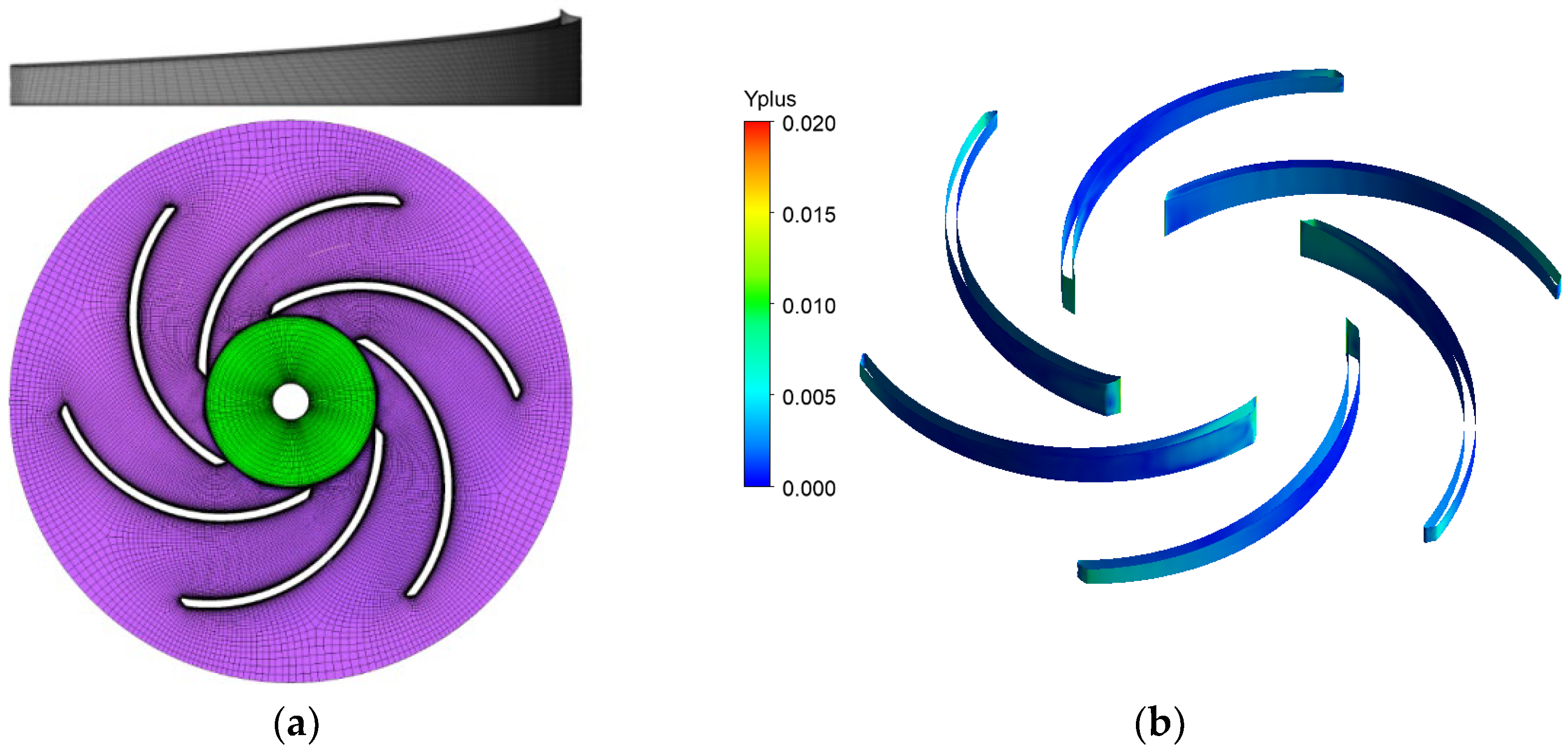
3.2. Meshing and Boundary Conditions

Figure 2a shows that in this study the TurboGrid 2019 R3 software was used to generate a high-quality hexahedral mesh and that the mesh around the blades was refined. Since the impeller domain has a circumferential symmetry and six blades, a single channel is meshed and then replicated six times in the circumferential direction. Mesh nodes connected to replication domains merge smoothly at the domain boundaries. The value of y⁺ in the whole impeller domain is less than 1, as shown in Figure 2b.

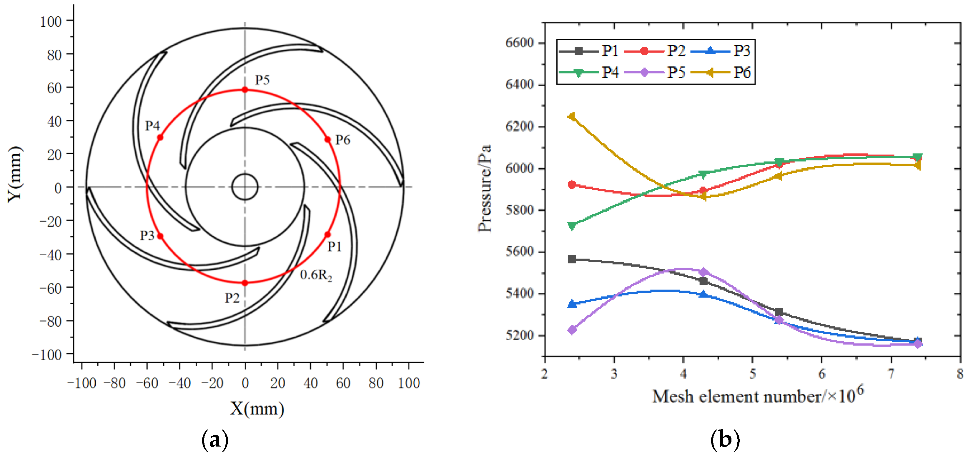
3.3. Mesh Independence Verification

The choice of mesh size should be such that the mesh density has no significant effect on the numerical simulation accuracy. Four mesh sizes (2.4 × 10⁶, 4.3 × 10⁶, 5.4 × 10⁶, 7.4 × 10⁶) were chosen to calculate the sensitivity of the grid number to the numerical simulation results. A value of 0.25Q_d shows a strong part-load and unstable operating condition, the head and efficiency of the pump may fluctuate significantly due to the influence of internal vortices. Therefore, the method of obtaining pressure data by setting monitoring points located inside the impeller will make the results more accurate. As shown in Figure 3a, six monitoring points are selected in the middle section of the impeller from the cross-sectional line of the radial position r/R₂ = 0.6. The differences in the numerical simulation results of the pressure values at each point for different numbers of meshes were analyzed. Figure 3b shows the pressure values at each point with different mesh numbers. When the grids have small numbers, the pressure values at the same point fluctuate considerably. But when the mesh number reaches 5.4 × 10⁶, the change in the pressure value is less than 4%. It shows that the flow field can be accurately predicted when the mesh number is 5.4 × 10⁶. To ensure accuracy and efficiency, the mesh size 5.4 × 10⁶ was chosen for the following numerical calculations.

The inlet boundary condition was set as total pressure, and the outlet boundary conditions was set as mass flow. The entire computational domain was discretized by the finite volume. Non-slip wall was set as the wall boundary condition. RNG k−ε, realizable k−ε, SST k−ω and LES are already available in ANSYS-Fluent. By employing the User Defined Function (UDF), the WA turbulence model was imported into ANSYS-Fluent. The time step in LES model calculation was set as 3.5 × 10⁻⁶ s, and the maximum iterations in each time step were 20, so as to ensure that the courant number was controlled within 1. To reach computational stability as soon as possible, the results of solving a steady flow field with the SST k−ω model were used as the initial flow field for the LES model calculation. The calculation results were recorded after 10 rotations of the impeller. The SIMPLEC algorithm was chosen to couple velocity and pressure. In all simulations, the residuals of the continuity and momentum equations, and the convergence criteria of the centrifugal pump head were set as 10⁻⁵.

3.4. Experimental Model

In the experiments at the Technical University of Denmark [4,32] PIV experiments were performed using CCD cameras, particle imaging velocimeters, pulsed laser emitters, image converters and synchronizers. PIV was performed on the horizontal (x, y) plane inside the impeller, which was located 2.9 mm above the plane hub, and on half of the impeller outlet width (Z/b₂ = 0.5). The locations of the two 93 × 94 mm² observation windows are shown in Figure 4.

4. Results and Discussion

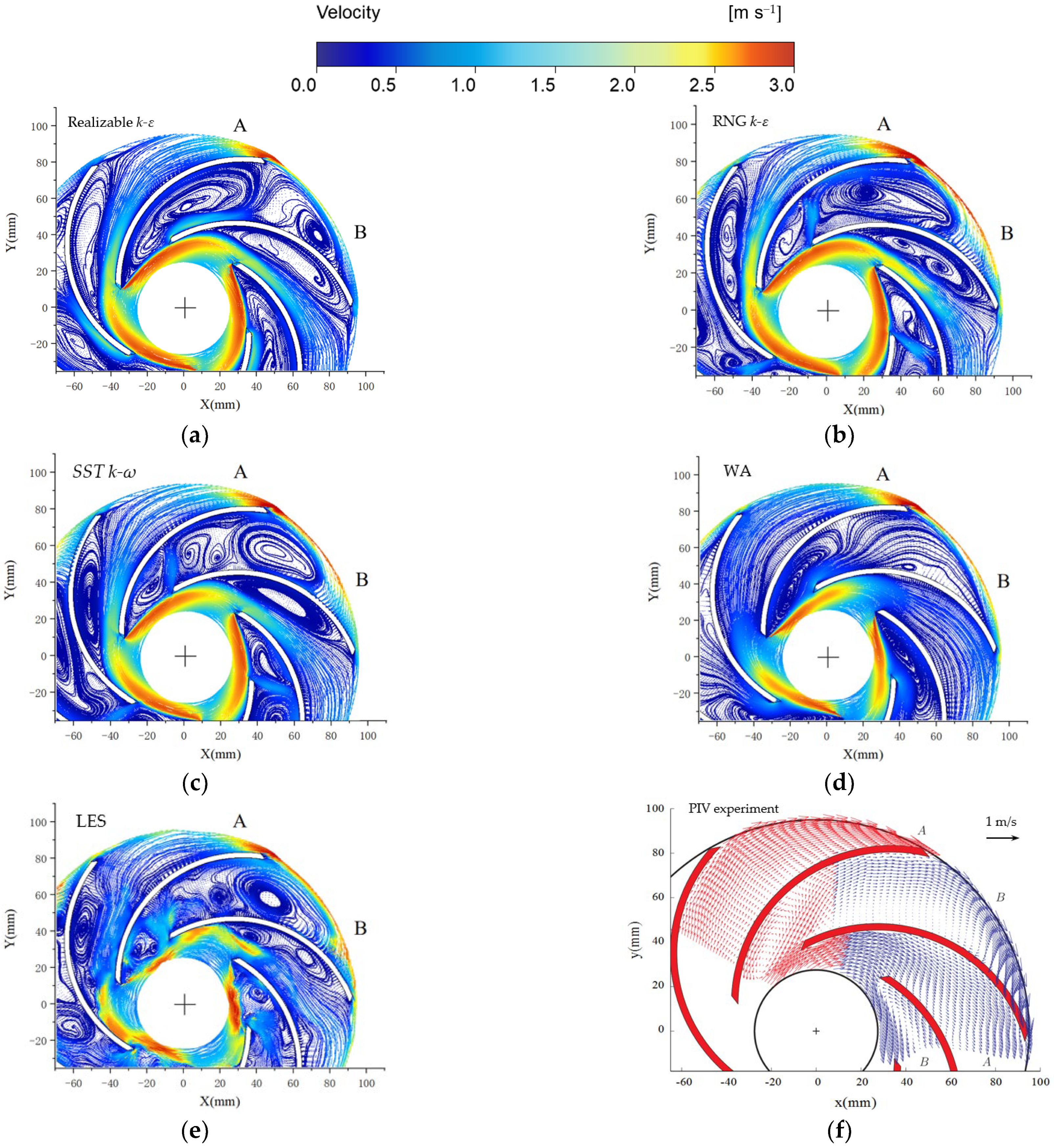
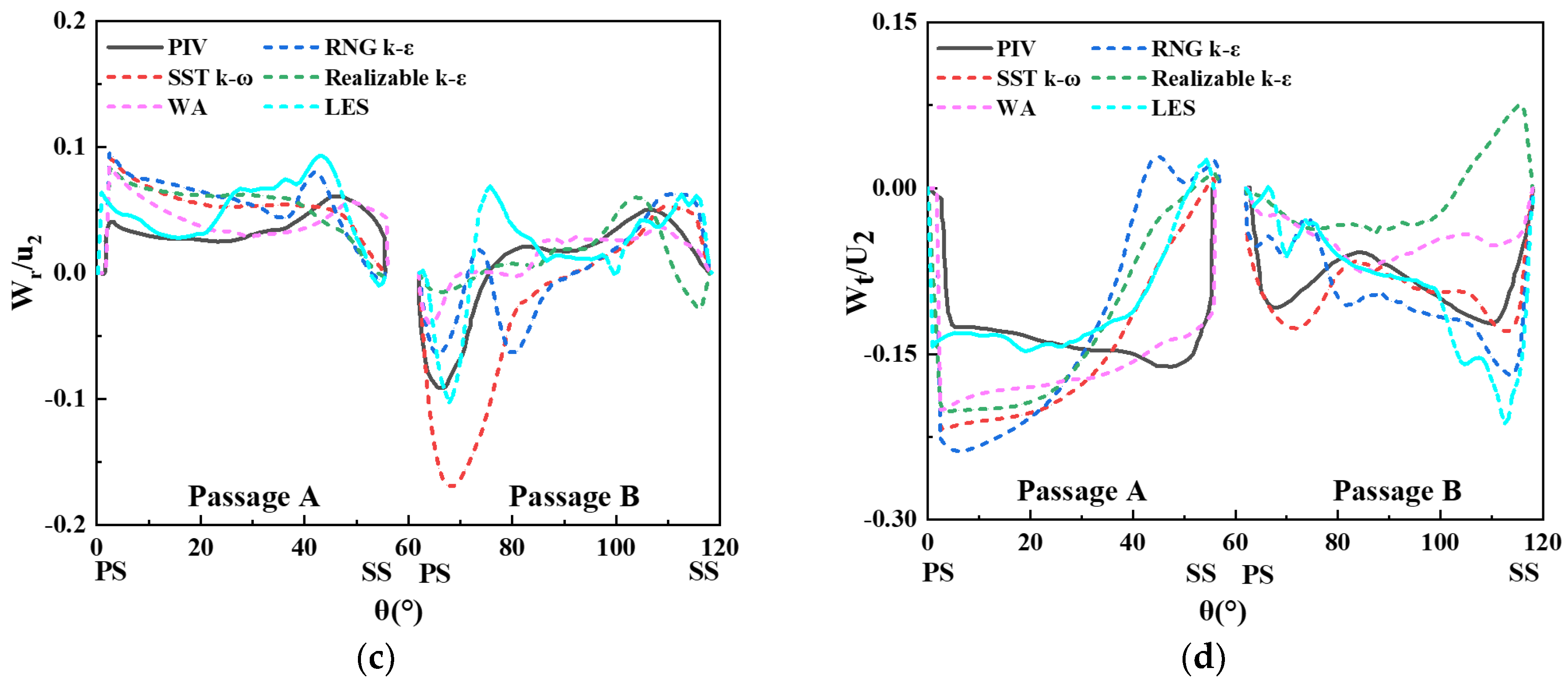
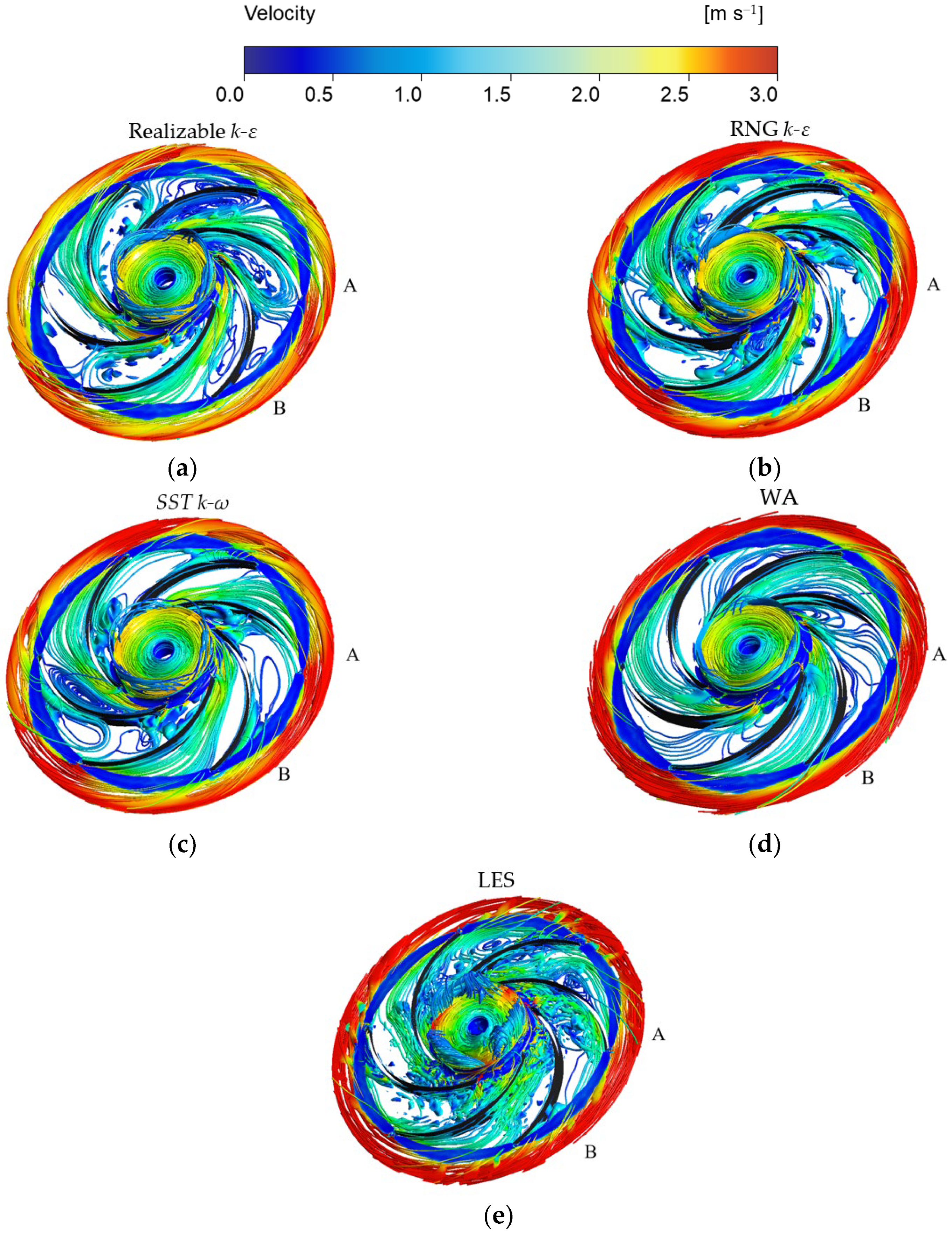
4.1. Internal Flow Field Analysis

Figure 5 is the streamline distribution on the impeller’s middle section using all four turbulence models and PIV experiments under a 0.25Q_d flow condition. Channel A is the non-stall channel and channel B is the stall channel. Under 0.25Q_d, the non-stall channel and stall channel in the impeller are distributed alternately. The flow in channel A is smooth and regular, and the streamlines are consistent with the blade profile. There are only a few mild flow separations around the blade surface. In channel B, there are two large stall cells. The stall cell can strongly block the inlet of this channel, resulting in the reduction in the flow capacity of this channel. Around the blade’s pressure surface, the stall cells occupy most of the area of the channel, and thereby push the fluid to the suction surface.

All models predict the alternating stall phenomenon successfully; however, they all show different flow field details. The realizable k−ε, RNG k−ε and SST k−ω models predict that the suction surface of channel A has a large stall cell, which is significantly different from the experimental results. The realizable k−ε model considerably overestimates the stall cell size at the entrance of channel B. The RNG k−ε and SST k−ω models overpredict the number of stall cells in channel B, but the streamlines in channel B have good agreement with the PIV results. The LES predicts smaller stalled cells on channel A, which is a small difference from the PIV test results. The LES model predicts flow in channel B in good agreement with the test data. The WA model predicts flow patterns very well in channel A, reaching almost the same values as in the PIV experiment. The number of stall cells in channel B and the separation flow point obtained from the WA model coincide well with the experiment, but the range of stall cells is slightly different from the experiment. In general, the LES and WA models have good agreement with the experiments. The WA model could accurately calculate the flow separation in the impeller under an adverse pressure gradient.

The relative velocity of different radial position r/R₂ at the impeller’s middle height was studied. As shown in Figure 6, the velocity value on the suction side in channel A predicted by the PIV is slightly larger than that on the pressure side. The reasons are twofold: one is that the stall cell at the entrance of channel B pushes a large amount of fluid into channel A; the other is that the internal flow is superimposed by the axial flow and a uniform flow [38]. The realizable k−ε, RNG k−ε, SST k−ω and LES models predict the presence of larger stall cells in channel A, with higher relative velocity values on the pressure side compared to the PIV experiment. In addition, the distribution of relative velocity values in channel B predicted by the four models, except for the WA model, are irregular. The relative velocity calculated using the WA model can match the experimental results, especially the simulation of the non-stall channel is in much better agreement with the experiment than the other models are.

Here, the velocity distribution obtained with the four turbulence models under a 0.25Q_d condition, the radial and tangential velocities at r/R₂ = 0.50 and 0.90 for each turbulence model, are analyzed. The positions of selected monitoring lines are as shown in Figure 7.

As shown in Figure 8, the velocity value on the suction side of channel A inlet is much higher than that on the pressure side. However, the calculation results of the three models realizable k−ε, RNG k−ε and SST k−ω are similar to each other but are contrary to the experiment. This significant difference is mainly attributed to the effect of inlet pre-rotation [37]. Under a small flow rate condition, the backflow generated by the rotation of the impeller combines with the leakage flow resulting in a large number of eddy currents at the inlet, and the influence of the eddy currents is ignored in the calculation process of these three models. The WA model considers the influence of the inlet eddy current, and the velocity distribution is very close to the experimental results. In channel B, all five models and experimentally obtained velocity maps show stall phenomena. The RNG k−ε, SST k−ω, LES and WA model results have good agreement with the PIV results with slightly different peaks.

The flow velocity at the exit of channel A is more uniform than at the entrance. The stall cell predicted by the realizable k−ε, RNG k−ε and SST k−ω models in channel A do not cover the exit; thus, the five models have achieved good prediction results. At the outlet of channel B, the radial velocities calculated using the SST k−ω, WA and LES models coincide well with PIV test in trend. In general, the LES and WA model results are closest to the PIV data for the velocity prediction in the entire impeller channel.

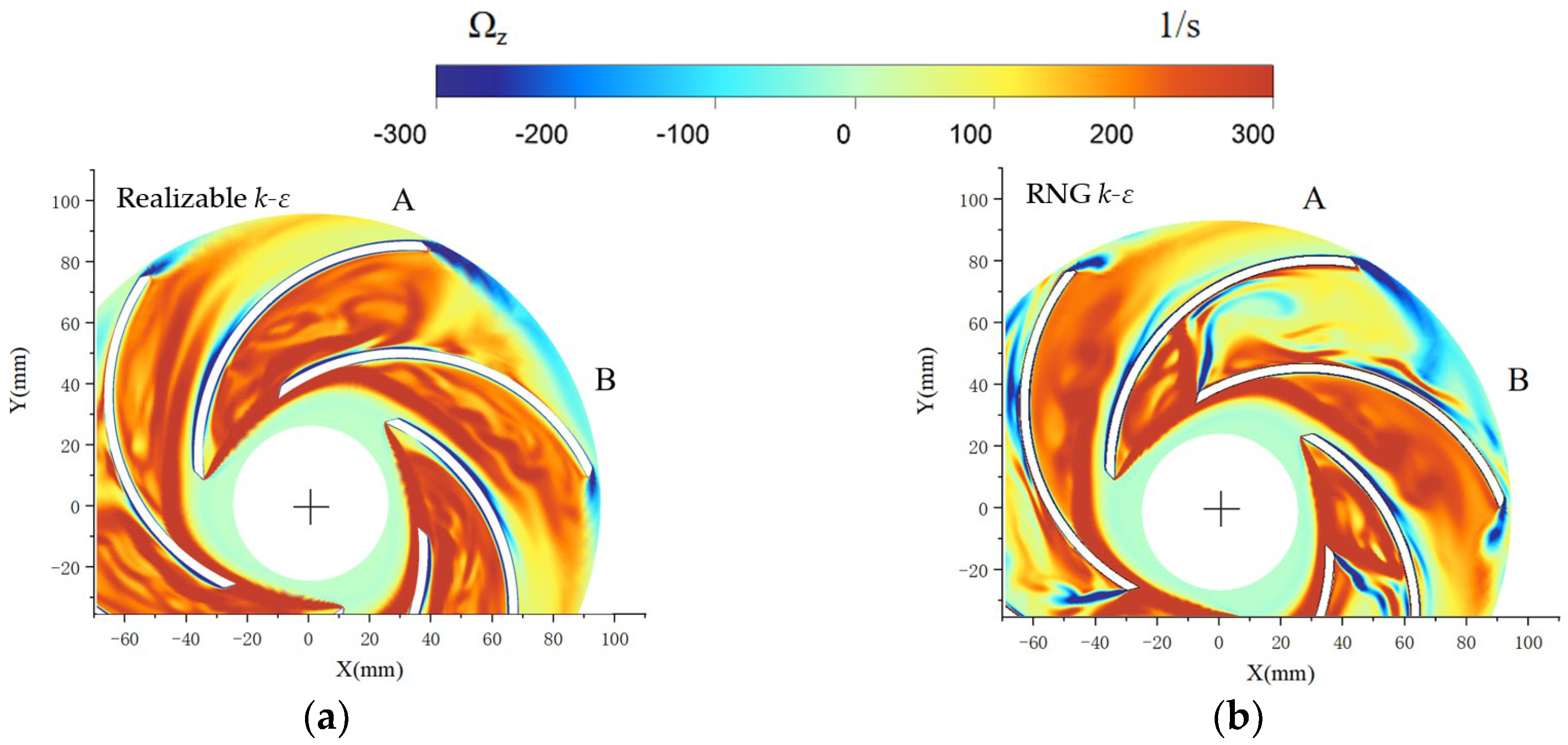
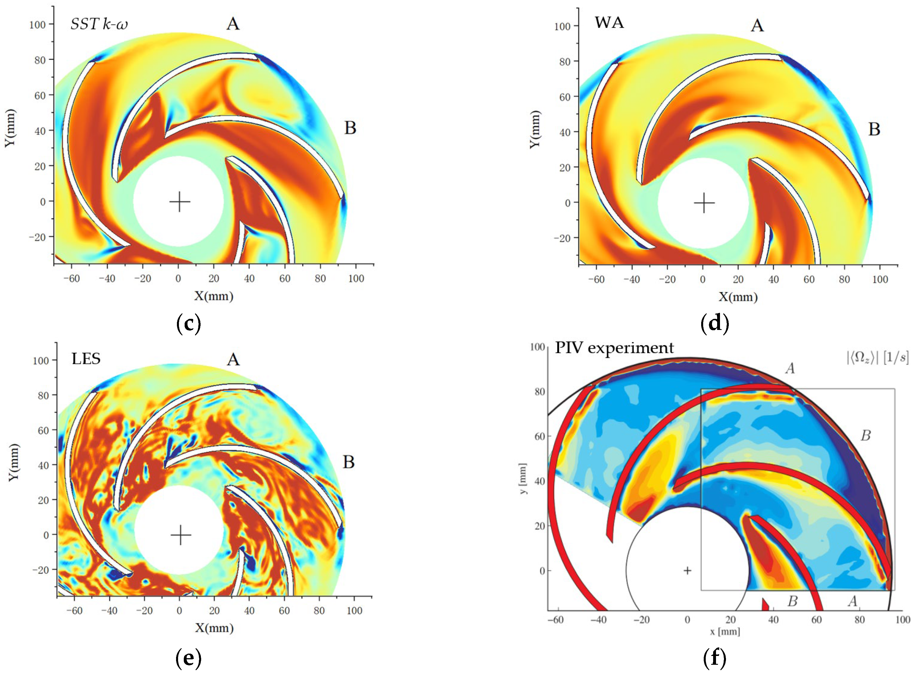
4.2. Vorticity and Vortex Intensity Analysis

Next, the five turbulence models are evaluated by computing the Z-directional vorticity magnitude. Figure 9 is a graph showing the intensity distribution of the Z-direction vorticity component. From Figure 9f [32] it can be observed that small stall cells shed from the impellers’ leading edge in channel A are distributed near the suction side of the blade and migrate downstream. In channel B, a small clockwise rotating vortex is shed from the pressure leading edge, and the area with high vorticity occupies the space of the impeller’s inlet. The five turbulence models successfully predict the two regions with high vorticity values in the non-stall channel, but the eddy rotation direction of the five models is opposite to that of the test in some ranges. The realizable k−ε model overestimates the two regions with high vorticity values and has the lowest agreement with the experiment. The predictions of the RNG k−ε, SST k−ω and LES models for the high vorticity region in channel B match well with the PIV data, but overestimate the range of stall vortices in channel A. The WA model has good agreement between the predicted vorticity value and the experiment, and the initial point and range of the stall cell are predicted successfully.

The distribution of the vortex structure in the stall cell was analyzed using the Q criterion [37]. The Q criterion can be defined as:

$$Q_c=\frac{1}{2}\left({\Omega }_{ij}{\Omega }_{ij}-c_q{S}_{ij}{S}_{ij}\right)$$

(16)

$${\Omega }_{ij}=\frac{1}{2}\left(\frac{\partial U_i}{\partial x_j}-\frac{\partial U_j}{\partial x_i}\right)$$

(17)

$$S_{ij}=\frac{1}{2}\left(\frac{\partial U_i}{\partial x_j}+\frac{\partial U_j}{\partial x_i}\right)$$

(18)

where Ω_ij is the rotation rate tensor, S_ij is the strain rate tensor, and c_q is the empirical coefficient (usually 1). When Ω_ij > S_ij, the rotational force on the fluid is greater than the stress force, and it is considered that there is a vortex structure present. The vortex intensity increases with an increase in Q_c.

The stall cells are analyzed using the Q_c iso-surface method. The value of the iso-surface has great influence on the expression of the stall cells. In order to express the internal vortex structure intuitively and clearly, a stall vortex of Q_c = 3000 1/s² was analyzed. The vortex structure and streamline diagram inside the impeller are shown in Figure 10. There are many stall cells gathering at the blade outlet, and the main reason for these vortex structures is the wake jet. For the realizable k−ε, RNG k−ε and SST k−ω models, the stall cells in stall channels are significantly more than those in non-stall channels. LES model recognition of vortex structures on the same iso-surface is more abundant, much more than by the other models. The inlet reflux vortex simulated by the WA model is located above the stall channels, while the simulation results of the other models are located above the non-stall channels.

5. Conclusions

A new one-equation WA model, three two-equation turbulence models, and LES were used to simulate the flow field inside a centrifugal pump impeller under deep stall conditions. The simulation results were compared with the PIV test results and the following conclusions can be drawn:

• Among the five turbulence models, LES has the best agreement with the experimental data. The WA model shows strong potential for accurately computing the stall. The reason is that the WA model adds a cross-diffusion term to the eddy viscosity R equation, so that the model can behave as a one-equation k−ω model in the near-wall region or as one-equation k−ε model away from the wall by employing a switching function. The WA model can also accurately predict flow separation under adverse pressure gradients.
• LES and the WA model are more accurate than the other models in simulating the flow patterns in the non-stall channel, with the results being highly consistent with the test data. The reason is that the other three models except the LES and WA model do not consider the effect of pre-rotation in the non-stall channel. The LES model predicts the best overlap of stall cell and velocity distribution in the stall channel with the PIV test results. The stall cell position predicted by the WA model is slightly different from that in the PIV experiment, but the calculation results are still better than those from the realizable k−ε, RNG k−ε and SST k−ω models.
• The Z-directional vorticity magnitudes predicted by all five models are slightly larger than the test data, but two regions with high vorticity values are successfully predicted. The WA model has good agreement with the experiment in predicting the size and range of stall cells in the non-stall channel; all other models have different degrees of overestimation. In general, the WA model can accurately predict the vorticity distribution in the impeller passage. The inlet reflux vortex simulated using the WA model is located above the stall channels, while the simulation results of other models are located above the non-stall channels. The LES model recognition of vortex structures on the same iso-surface is better.

References

1. Emmons, H.; Pearson, C.; Grant, H. Compressor surge and stall propagation. Trans. Am. Soc. Mech. Eng. 1995, 77, 455–467. [Google Scholar] [CrossRef]
2. Li, W.; Yang, Z.; Shi, W.; Li, E.; Ji, L. Research progress of non-uniform inflow of water jet pump. J. Drain. Irrig. Mach. Eng. 2022, 40, 757–765. [Google Scholar]
3. Krause, N.; Zähringer, K.; Pap, E. Time-resolved particle imaging velocimetry for the investigation of rotating stall in a radial pump. Exp. Fluids 2005, 39, 192–201. [Google Scholar] [CrossRef]
4. Pedersen, N.; Larsen, P.; Jacobsen, C. Flow in a centrifugal pump impeller at design and off-design conditions—Part I: Particle image velocimetry (PIV) and laser Doppler velocimetry (LDV) measurements. J. Fluids Eng. 2003, 125, 61–72. [Google Scholar] [CrossRef]
5. Ullum, U.; Wright, J.; Dayi, O.; Ecder, A.; Soulaimani, A.; Piché, R.; Kamath, H. Prediction of rotating stall within an impeller of a centrifugal pump based on spectral analysis of pressure and velocity data. J. Phys. Conf. Ser. 2006, 52, 36–45. [Google Scholar] [CrossRef]
6. Liu, T.; Zhang, Y.; Du, X. A review of rotating stall of pump turbines. J. Hydroelectr. Eng. 2015, 34, 16–24. [Google Scholar]
7. Zhao, B.; Liu, Y.; Han, L.; Cao, K.; Chen, H.; Huang, Z. Vortex identification and its evolution law of mixed-flow pump under low-flow condition. J. Drain. Irrig. Mach. Eng. 2023, 41, 231–238. [Google Scholar]
8. Zhang, N.; Yang, M.G.; Gao, B. Unsteady rotating stall characteristics in a centrifugal pump with slope volute at low flow rates. J. Vib. Shock 2015, 34, 189–194. [Google Scholar]
9. Tang, P.; Li, H.; Issaka, Z.; Chen, C. Effect of manifold layout and fertilizer solution concentration on fertilization and flushing times and uniformity of drip irrigation systems. Agric. Water Manag. 2018, 200, 71–79. [Google Scholar] [CrossRef]
10. Issaka, Z.; Li, H.; Jiang, Y.; Tang, P.; Chao, C. Comparison of rotation and water distribution uniformity using dispersion devices for impact and rotary sprinklers. Irrig. Drain. 2019, 68, 881–892. [Google Scholar] [CrossRef]
11. Zhou, L.; Bai, L.; Li, W.; Shi, W.; Wang, C. PIV validation of different turbulence models used for numerical simulation of a centrifugal pump diffuser. Eng. Comput. 2018, 35, 2–17. [Google Scholar] [CrossRef]
12. Yang, Y.; Zhou, L.; Shi, W.; He, Z.; Han, Y.; Xiao, Y. Interstage difference of pressure pulsation in a three-stage electrical submersible pump. J. Pet. Sci. Eng. 2021, 196, 107653. [Google Scholar] [CrossRef]
13. Zhou, L.; Hang, J.; Bai, L.; Krzemianowski, Z.; El-Emam, M.A.; Yasser, E.; Agarwal, R. Application of entropy production theory for energy losses and other investigation in pumps and turbines: A review. Appl. Energy 2022, 318, 119211. [Google Scholar] [CrossRef]
14. Innocenti, A.; Jaccod, A.; Popinet, S.; Chibbaro, S. Direct numerical simulation of bubble-induced turbulence. J. Fluid Mech. 2021, 918, A23. [Google Scholar] [CrossRef]
15. Tucker, P. Unsteady Computational Fluid Dynamics in Aeronautics; Springer Science & Business Media: Berlin/Heidelberg, Germany, 2014; 104p. [Google Scholar]
16. Smagorinsky, J. General circulation experiments with the primitive equations: I. Basic Exp. Mon. Weather Rev. 1963, 91, 99–164. [Google Scholar] [CrossRef]
17. Li, W.; Zhou, L.; Shi, W.; Ji, L.; Yang, Y.; Zhao, X. PIV experiment of the unsteady flow field in mixed-flow pump under part loading condition. Exp. Therm. Fluid Sci. 2017, 83, 191–199. [Google Scholar] [CrossRef]
18. El-Emam, M.; Zhou, L.; Yasser, E.; Bai, L.; Shi, W. Computational methods of erosion wear in centrifugal pump: A state-of-the-art review. Arch. Comput. Methods Eng. 2022, 29, 3789–3814. [Google Scholar] [CrossRef]
19. Wilcox, D.C. Turbulence Modeling for CFD; D.C.W. Industries: La Canada, CA, USA, 1998; pp. 103–217. [Google Scholar]
20. Zhang, Y.; Zang, W.; Zheng, J.; Cappietti, L.; Zhang, J.; Zheng, Y.; Fernandez-Rodriguez, E. The influence of waves propagating with the current on the wake of a tidal stream turbine. Appl. Energy 2021, 290, 116729. [Google Scholar] [CrossRef]
21. Mousavi, S.; Hosseini, K.; Fouladfar, H.; Mohammadian, M. Comparison of different turbulence models in predicting cohesive fluid mud gravity current propagation. Int. J. Sediment Res. 2020, 35, 504–515. [Google Scholar]
22. Chen, Q. Prediction Performance of Several Turbulence Models in Flows Pertinent to Turbomachinery. Master’s Thesis, Tsinghua University, Beijing, China, 2007. [Google Scholar]
23. Zhang, W. Analysis and Predicition of the Internal Flow in the Vane Pump Impeller at Off Design Condition. Ph.D. Thesis, Shanghai University, Shanghai, China, 2010. [Google Scholar]
24. Ji, L.; Li, W.; Shi, W.; Agarwal, R. Application of Wray–Agarwal turbulence model in flow simulation of a centrifugal pump with semispiral suction chamber. ASME J. Fluids Eng. 2021, 143, 031203. [Google Scholar] [CrossRef]
25. Han, X.; Rahman, M.; Agarwal, R. Development and application of wall-distance-free Wray-Agarwal turbulence model. In Proceedings of the AIAA Aerospace Sciences Meeting, Kissimmee, FL, USA, 8–12 January 2018. [Google Scholar]
26. Wray, T.; Agarwal, R. Low-Reynolds-number one-equation turbulence model based on kω closure. AIAA J. 2015, 53, 2216–2227. [Google Scholar] [CrossRef]
27. Yang, H.; Agarwal, R. CFD simulations of a triangular airfoil for Martian atmosphere in low-reynolds number compressible flow. In Proceedings of the AIAA Aviation 2019 Forum, Dallas, TX, USA, 17–21 June 2019. [Google Scholar]
28. Wray, T.J. Development of a One-Equation Eddy Viscosity Turbulence Model for Application to Complex Turbulent Flows; Washington University: St. Louis, MO, USA, 2016. [Google Scholar]
29. Rahman, M.; Agarwal, R.; Siikonen, T. RAS one-equation turbulence model with non-singular eddy-viscosity coefficient. Int. J. Comput. Fluid Dyn. 2016, 30, 89–106. [Google Scholar] [CrossRef]
30. Han, Y.; Zhou, L.; Bai, L.; Shi, W.; Agarwal, R. Comparison and validation of various turbulence models for U-bend flow with a magnetic resonance velocimetry experiment. Phys. Fluids 2021, 33, 125117. [Google Scholar] [CrossRef]
31. Ouyang, Y.; Tang, K.; Xiang, Y.; Zou, H.; Chu, G.; Agarwal, R.K.; Chen, J.F. Evaluation of various turbulence models for numerical simulation of a multiphase system in a rotating packed bed. Comput. Fluids 2019, 194, 104296. [Google Scholar] [CrossRef]
32. Pedersen, N. Experimental Investigation of Flow Structures in a Centrifugal Pump Impeller Using Particle Image Velocimetry. Ph.D. Thesis, Technical University of Denmark, Lyngby, Denmark, 2000. [Google Scholar]
33. Zhang, W.; Yu, Y.; Chen, H. Numerical simulation of flow in centrifugal pump Impeller at off-design conditions. J. Drain. Irrig. Mach. Eng. 2010, 1, 38–42. [Google Scholar]
34. Wen, T.; Agarwal, R.K. A new extension of wray-agarwal wall distance free turbulence model to rough wall flows. In Proceedings of the AIAA Scitech 2019 Forum, San Diego, CA, USA, 7–11 January 2019. [Google Scholar]
35. Germano, M.; Piomelli, U.; Moin, P.; Cabot, W. A dynamic subgrid-scale eddy viscosity model. Phys. Fluids A Fluid Dyn. 1991, 3, 1760–1765. [Google Scholar] [CrossRef]
36. Lilly, D.K. A proposed modification of the Germano subgrid-scale closure method. Phys. Fluids A: Fluid Dyn. 1992, 4, 633–635. [Google Scholar] [CrossRef]
37. Byskov, R.; Jacobsen, C.; Pedersen, N. Flow in a centrifugal pump impeller at design and off-design conditions—Part II: Large eddy simulations. J. Fluids Eng. 2003, 125, 73–83. [Google Scholar] [CrossRef]
38. Feng, J.; Wang, C.; Luo, X. Rotating stall in centrifugal pump impeller under part-load conditions. J. Hydroelectr. Eng. 2018, 37, 117–124. [Google Scholar]
Figure 1. Impeller model.
Water 15 03432 g001
Figure 2. Mesh of the impeller and y+ distribution on the blades. (a) Structured mesh in the impeller; (b) y+ distribution.
Water 15 03432 g002
Figure 3. Mesh independence of solution analysis. (a) Position of monitoring point; (b) pressure changes with different mesh numbers.
Water 15 03432 g003
Figure 4. Schematic diagram of test position and observation windows in experiment [4,32].
Water 15 03432 g004
Figure 5. Comparisons of the streamline distribution at the impeller’s middle section. (a) Realizable kε; (b) RNG k−ε; (c) SST k−ω; (d) WA; (e) LES; (f) PIV experiment [4,32].
Water 15 03432 g005
Figure 6. Velocity field of z/b2 = 0.5 and r/R2 = {0.50, 0.65, 0.75, 0.90}. (a) Realizable k−ε; (b) RNG k−ε; (c) SST k−ω; (d) WA; (e) LES; (f) PIV experiment [4,32].
Water 15 03432 g006
Figure 7. The positions of selected monitoring lines.
Water 15 03432 g007
Figure 8. Radial and tangential velocities. (a) Radial velocity (z/b2 = 0.5, r/R2 = 0.5); (b) tangential velocity (z/b2 = 0.5, r/R2 = 0.5); (c) radial velocity (z/b2 = 0.5, r/R2 = 0.9); (d) tangential velocity (z/b2 = 0.5, r/R2 = 0.9).
Water 15 03432 g008aWater 15 03432 g008b
Figure 9. Z-directional vorticity magnitude. (a) Realizable k−ε; (b) RNG k−ε; (c) SST k−ω; (d) WA; (e) LES; (f) PIV experiment [4,32].
Water 15 03432 g009aWater 15 03432 g009b
Figure 10. Iso-surface of the vortex structure inside the impeller (Qc = 3000 1/s2). (a) Realizable k−ε; (b) RNG k−ε; (c) SST k−ω; (d) WA; (e) LES.
Water 15 03432 g010