Article

Analysis of Debris Flow Damage Using High-Resolution Topographical Data

Department of Urban Environment & Disaster Management, Graduate School of Disaster Prevention, Kangwon National University, 346 Joongang-ro, Samcheok-si 25913, Republic of Korea
*
Author to whom correspondence should be addressed.
Water 2023, 15(19), 3454; https://doi.org/10.3390/w15193454
Submission received: 29 August 2023 / Revised: 27 September 2023 / Accepted: 28 September 2023 / Published: 30 September 2023

Abstract

:
Mountain disasters, such as landslides and debris flows, are becoming more prevalent due to abnormal weather patterns. Debris flows, triggered by heavy rainfall, are causing escalating damage to residential areas and roads as they surge down mountain streams. In order to both mitigate this damage and comprehend the underlying causes of such mountain disasters, comprehensive field investigations were carried out in regions where debris flows had transpired. To establish spatial information for analyzing vulnerable areas, GIS data were employed. Additionally, precise measurements of the actual extent of debris flow in targeted zones were obtained through the utilization of terrestrial LiDAR scanning. Subsequently, the process of debris flow was replicated using FLO-2D, a numerical model designed for such scenarios. This simulation incorporated actual rainfall data that had precipitated debris flow incidents, as well as probability-based rainfall data corresponding to return periods of 30, 50, and 100 years. Key parameters, including flow depth, velocity, and diffusion area, were compared across different scenarios. The sedimentation area of the section where debris flow originated, as determined from terrestrial LiDAR scan data, was estimated to be approximately 21,300 square meters. The outcomes of the FLO-2D simulation revealed that the diffusion area for Case I was approximately 20,900 m2, while the simulated diffusion area for a 100-year return period was calculated to be 40,725 m2. Furthermore, flow depth, velocity and diffusion area exhibited a gradual incremental trend in simulation results.

1. Introduction

In recent years, there has been a notable surge in disasters linked to abnormal climatic conditions, particularly in mountainous areas. These regions have witnessed a heightened frequency of intense rainfall events, leading to an increase in occurrences of debris flows and significant damage to downstream residences and transportation infrastructure. Among these vulnerable areas, Gangwon-do stands out, with approximately 80% of its terrain composed of mountains, making it exceptionally susceptible to landslides and debris flows compared to other parts of the country. Debris flows typically manifest in the wake of heavy rainfall or typhoons, primarily affecting natural slopes and mountain valleys. These events are characterized by their substantial scale, rapid flow velocities, and the mixture of sediment and water they carry downstream.
Understanding the potential triggers of debris flows and similar hazardous events is critical to mitigating their impacts and managing mountainous regions efficiently. The cornerstone of a proactive strategy to deal with debris flow disasters is the accurate prediction of their location and timing, as well as quantitative assessments of their path, volume, erosion and sediment deposition. It is worth noting that steep terrain is particularly susceptible to landslides and debris flows, and the impact of these events on road infrastructure can be particularly devastating [1]. The acquisition of spatial data is therefore essential to the analysis of disasters in mountainous areas. The production of accurate topographic information plays a key role in ensuring the accuracy and effectiveness of these analyses.
Ongoing research endeavors are actively focused on the prediction of landslides and debris flows while simultaneously minimizing their destructive impacts. Various methodologies, encompassing rheology and erosion–sedimentation models, have been extensively employed to delve deeper into the intricate dynamics underpinning debris flows [2,3,4,5,6,7]. Research efforts in landslide prediction and impact mitigation are currently employing a combination of deterministic and probabilistic approaches.
Deterministic methodology has proven to be a valuable tool for disaster prediction when precise initial conditions and parameters have been accurately recorded. This approach heavily relies on accurate initial topographic information and precipitation data to model the probability of landslides. Importantly, it employs statistical analysis and numerical model evaluation using field data as essential tools for a systematic response to mitigate the risks associated with debris flows. This methodology predicts the susceptibility of steep areas to landslides during rainfall [8,9], conducts GIS-based landslide risk assessments using deterministic modeling [10], and employs simulations like FLO-2D. It also introduced a numerical method to simulate the behavior of landslides and debris flows in a two-dimensional channel [11,12,13,14]. Furthermore, researchers have replicated the dynamic process of disasters and established landslide hazard zones through numerical simulation and risk assessment to more accurately identify landslide-prone areas [15,16]. Although these methodologies significantly contribute to landslide prediction, they inherently entail uncertainties due to simplifications and assumptions.
Probabilistic methodologies, on the other hand, priorities uncertainty in landslide and debris flow prediction. These approaches address uncertainty in initial conditions and parameters by modeling various variables, including topographic, meteorological, and geological variables, as probability distributions. Introduced the FORM (First Order Reliability Method) method, a probabilistic approach to geotechnical design, and assessed safety taking into account ground uncertainty. In addition, a probabilistic method for evaluating soil displacement on seismically loaded slopes was investigated. Researchers have emphasized the importance of carrying out GIS-based probabilistic analyses that can holistically consider the various factors contributing to landslide risk, using GIS-FORM to assess slope collapse risk [17,18,19]. Debris flow risk assessment and the identification of high-risk areas are vital components of disaster prevention and mitigation strategies in mountainous regions. In this context, a probabilistic assessment has been conducted to evaluate the potential risks associated with roads situated in close proximity to mountain slopes [20].
In this research, we use the FLO-2D numerical model to perform a debris flow analysis, emphasizing the critical role of the model in predicting debris flow disasters and assessing associated risks. In a previous study, FLO-2D numerical simulations were performed for areas where debris flow disasters occurred, and the simulation results were compared with field data to verify the accuracy of the model predictions [11,15]. In order to understand the dynamics of debris flow material as influenced by rainfall, analyses have been carried out to assess the sensitivity of the models to parameter changes and to predict the extent of debris flow diffusion [12,14]. The simulations also highlight the importance of using LiDAR DEM to improve the accuracy and reliability of predictions of debris flow occurrence, movement and erosion [21]. In numerical modeling studies, achieving a close match with real-world phenomena is of paramount importance. While the above studies have shown consistency between debris flow patterns and model fit, quantitative data on the affected areas are still lacking. Consequently, uncertainties remain regarding the extent of debris flow diffusion. To comprehensively overcome these limitations, our study carefully integrates various data sources, including field data, parameters, LiDAR DEM and more. In addition, we conducted a topographic LiDAR survey to fill in the quantitative data gaps, thus enabling a quantitative representation and analysis of the debris flow-affected areas.
Previous research has mainly focused on investigating the causal factors of debris flows and analyzing relevant models, often neglecting the use of accurate topographic data. Our study aims to bridge this gap. We have meticulously surveyed the areas affected by debris flows using LiDAR survey technology, enabling us to construct a high-resolution topographic dataset. The FLO-2D model was used to visualize debris flow characteristics and assess downstream risk, analyzing key parameters such as flow depth, velocity and diffusion area, and allowing a comprehensive comparison of spread areas at different flow rates. However, it is important to emphasize that our results and methodology are based on specific case studies and inherently involve modeling and associated uncertainties. Consequently, further research is warranted to validate their applicability in regions characterized by unique topographic and climatic conditions.

2. Methods

2.1. Study Area and Field Survey

The study area is situated in Seorak-ro, Buk-myeon, Inje-gun, Gangwon-do, specifically encompassing Jangsu Bridge 5 and National Road No. 44 within Seoraksan National Park, as depicted in Figure 1. In 2006, a substantial debris flow event transpired due to heavy rainfall triggered by Typhoon Ewinia. This event led to a concentrated collapse of terrain primarily along National Road 44, which traverses Seoraksan National Park in an east–west direction. The torrential inflow of water inundated rivers in a sudden surge, resulting in severe damage to numerous homes and crops. Within the Hangyecheon basin portion of Seoraksan National Park, a historical record of debris flow exists in its natural state, rendering it relatively accessible. Through a comprehensive enumeration survey, it was determined that the flow distance from the origin of the debris flow to the sedimentary region amounted to approximately 2 km. The initiation area was characterized by steep slopes and the presence of significant-sized boulders. The dominant path of the debris flows followed the course of the valley, causing substantial erosion, exceeding 2 m, along both sides of the valley’s lower reaches, as shown in Figure 2. A protective ring net was established within the sedimentary area. Over time, however, this net became ineffective as it became filled with soil, subsequently losing its runoff reduction functionality. In the event of additional debris flow incidents, this region poses a significant threat, carrying the potential for substantial damage to bridges and small rivers located downstream.
The amount of rainfall during the debris flow event is illustrated in Figure 3. Over the course of a week, the cumulative rainfall amounted to 625 mm, surpassing 50% of the region’s average annual precipitation of 1210 mm. In the three days leading up to the debris flow incident, the cumulative rainfall amounted to 257 mm, resulting in highly saturated soil conditions due to the preceding downpours. In this study, we conducted FLO-2D analysis employing actual rainfall data corresponding to the day of the debris flow event. For comparative purposes, we utilized probability-based rainfall data specific to the Inje area, sourced from the Ministry of Land, Transport and Maritime Affairs (2011), as presented in Table 1. The simulation was performed using data with recurrence periods of 30, 50, and 100 years and durations of 60 min. The peak flow for debris flow, according to the numerical simulations, was calculated using Equation (1), with reference to a report [22] that provided a method for estimating discharge in small-scale watersheds.
Q = 0.2778 C I A
where Q represents the flow rate at the basin outlet, while C denotes the runoff coefficient contingent upon soil composition. The prescribed runoff coefficient calculation criteria established by the Korea Forest Service were adhered to, with a value of 0.5 employed to accommodate the steep slopes characteristic of mountainous terrains. In addition, I is the rainfall intensity and A is the area of the watershed.

2.2. Terrestrial LiDAR

To classify and assess the pre- and post-disaster conditions of debris flow within the affected region, and to quantify the extent of debris flow dispersion, terrestrial LiDAR technology was employed. A LiDAR scanning operation was executed, covering a distance of approximately 1.5 km from the sediment accumulation zone to the initial point of the debris flow, tracing along the course of the valley line. Terrestrial LiDAR operates on the principle of emitting laser light towards a measurement object, such as the terrain or relevant features, and then capturing and analyzing the reflected laser light using a light-detection sensor. This system comprises a transmitter, a receiver, and a processor. The LiDAR system possesses a maximum measurement range of 650 m, yielding points with a precision error of 15 mm within vertical angles ranging from 0° to 80° and horizontal angles spanning 0° to 360°. Figure 4a shows the LiDAR measuring device employed. Terrestrial LiDAR technology allows the collection of highly accurate elevation data covering terrain features, roads and infrastructure elements. The acquisition process involves collecting coordinates and scan data from a designated region of interest. The gathered data undergo processing in a point-based format, ultimately leading to the generation of a point cloud utilizing specialized post-processing software. This point cloud corresponds to the depiction showcased in (b). To ensure precision in altitude representation, a filtration procedure is executed to eliminate elements such as trees and rocks, retaining solely the points that accurately represent the terrain. This refined terrain data are depicted in (c). Subsequently, the point cloud serves as the foundational material from which an exacting Digital Elevation Model (DEM) is meticulously fashioned.

2.3. FLO-2D

The FLO-2D model [3] is a grid-based numerical modeling software specifically designed for simulating flood and debris flow phenomena. This modeling tool is particularly effective when it comes to capturing the intricate interplay between the movement of debris flow and water flow. It proves valuable in assessing the risk associated with debris flow incidents due to its capability to predict essential parameter variables crucial for gauging the intensity during the progression of debris flow movement. These variables encompass parameters like runout distance, volume of sediment accumulation, flow velocity, and depth. As a useful tool for simulating debris flow disaster areas and preventing disaster risk in conjunction with GIS and other applications, the FLO-2D model is defined in eight flow directions in a plane, and the continuity equation and equation of motion in each direction are configured as shown in Equations (2)–(4) [23].
h t + v h x + v h y = i ,
S f x = S a x h x v x g v x x v y g v x y 1 g v x t
S f y = S a y h y v y g v y y v x g v y x 1 g v y t
where h is the flow depth, v x ,   v y is the x and y axis velocity at mean water depth, i is the rainfall intensity, S f is the total friction slope, S a in the bed slope, and g is the gravitational acceleration. Unlike general fluids, the high-density debris flow shear stress can be expressed as Equation (5).
= τ y + η v y + C v y 2
where τ is the shear stress, τ y is the Mohr–Coulomb shear resistance, τ v is the viscous shear stress, τ t is the turbulent shear stress and τ d   is the dispersive shear stress,   η is the dynamic viscosity coefficient and C is the internal shear coefficient. Integrating the total shear stress with respect to the flow depth is given in Equation (6).
S f = S y + S v + S t d = T y γ m h + K η u 8 γ m n 2 + n 2 u 2 n 4 / 3
where S f is the total friction slope, S y is the yield slope, S v is the viscosity slope, S t d is the turbulence-dispersion slope, γ m is the specific weight of the sediment mixture, K is the resistance parameter and n is the value of Manning’s coefficient. Depending on the yield stress τ y , viscosity η and volume concentration C v , we can express these relationships through Equations (7) and (8). α i and β i are empirical coefficients established through experimentation.
τ y = α 1 e β 1 C v
η = α 2 e β 2 C v
For the FLO-2D simulation, the yield stress and viscosity values are experimental empirical coefficients classified according to the topographic conditions of the basin [3] in Table 2, and the laminar flow resistance (K) is shown in Table 3 according to the conditions of the ground surface, and the appropriate values for the target basin are applied as shown in Table 4.

3. Terrain Data and FLO-2D Simulation Analysis

3.1. Characteristic of Terrain Data

To comprehensively assess the topographical attributes of the target basin, an extensive topographical analysis was conducted employing digital elevation data at a spatial resolution of 5 m × 5 m. The basin’s expanse spans approximately 1.23 km2. In Figure 5a, the basin’s elevation ranges between 510 and 1280 m, exhibiting a pronounced disparity in altitudes. In (b), the upstream area where the debris flow transpired, slopes exceeding 40° were prevalent. The overall basin exhibited an average slope of 31°, with the steepest incline reaching 67°, rendering it a classification of high terrain gradient. In (c), the soil map is predominantly OdF, and the topsoil in this area is brown loam, while the subsoil is yellow-brown gravel or stony sandy loam. The soil parent material consists of weathered residual layers of granite and schist, and it is distributed on steep slopes. In addition, (d) the geological composition primarily featured gneiss and granite formations.
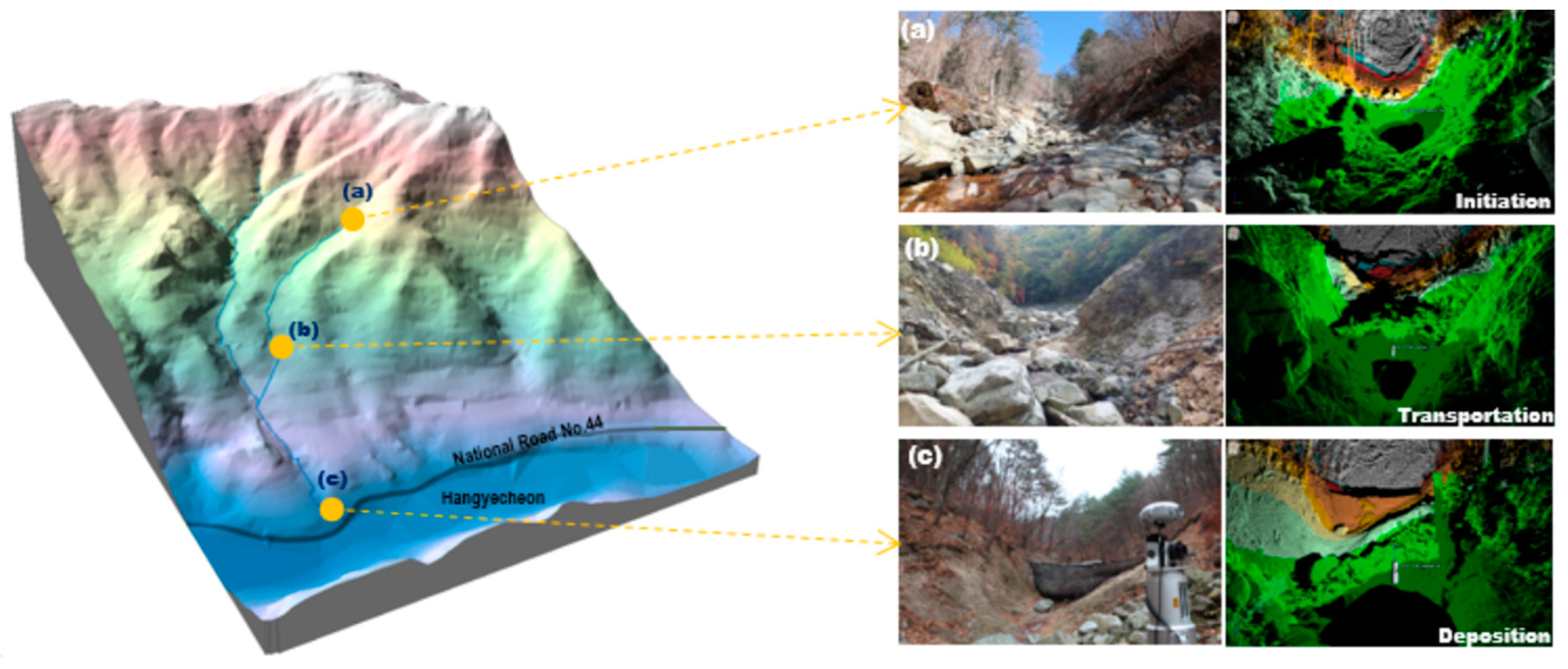
To assess the risk associated with a debris flow disaster, an extensive field survey was conducted, accompanied by terrestrial LiDAR scanning along the affected area. Figure 6 encompasses site photographs and LiDAR scan data, each representing the initiation, transportation, and deposition stages of the debris flow process. The span between the initiation point (a) and the deposition area (c), where the debris flow occurred, measures approximately 1.5 km. Comparative analysis between pre- and post-disaster digital maps and LiDAR measurements facilitated the observation of alterations in the terrain. Notably, the initiation area featured an exceedingly steep slope, and during the transportation phase, substantial erosion of approximately 2 m transpired on both sides of the valley. At sedimentary location (c), a protective ring net was installed to impede the outflow of debris flow. However, this net has become filled with debris, rendering its runoff-reducing capacity ineffective.
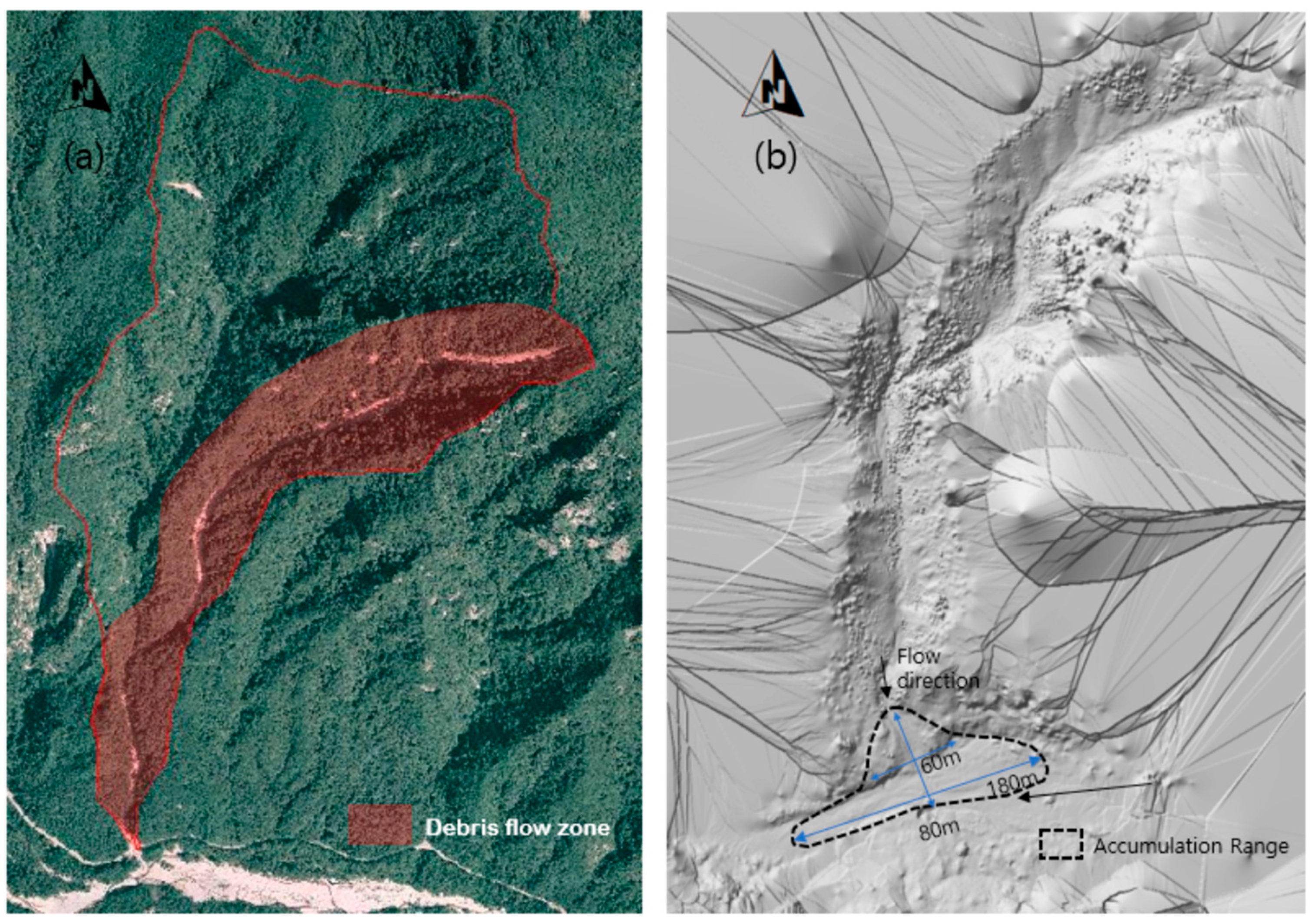
The geographic data obtained through digital map and LiDAR scans underwent processing to determine the extent of debris flow diffusion subsequent to the disaster. These data were subsequently employed as a reference for numerical simulation comparisons. In Figure 7a, an aerial photograph taken immediately after the debris flow catastrophe highlights the area designated in red as the region affected by the debris flow. In Figure 7b, the LiDAR-measured point data were transformed into a Digital Elevation Model (DEM), serving as the foundation for estimating the sedimentation (diffusion) area downstream. By comparing the LiDAR data with the numerical map, the spread area of the debris flow was determined. This analysis yielded a calculated debris flow spread area of approximately 21,300 m2. This value was subsequently employed as a reference for comparison with data obtained from numerical model simulations.

3.2. FLO-2D Simulation

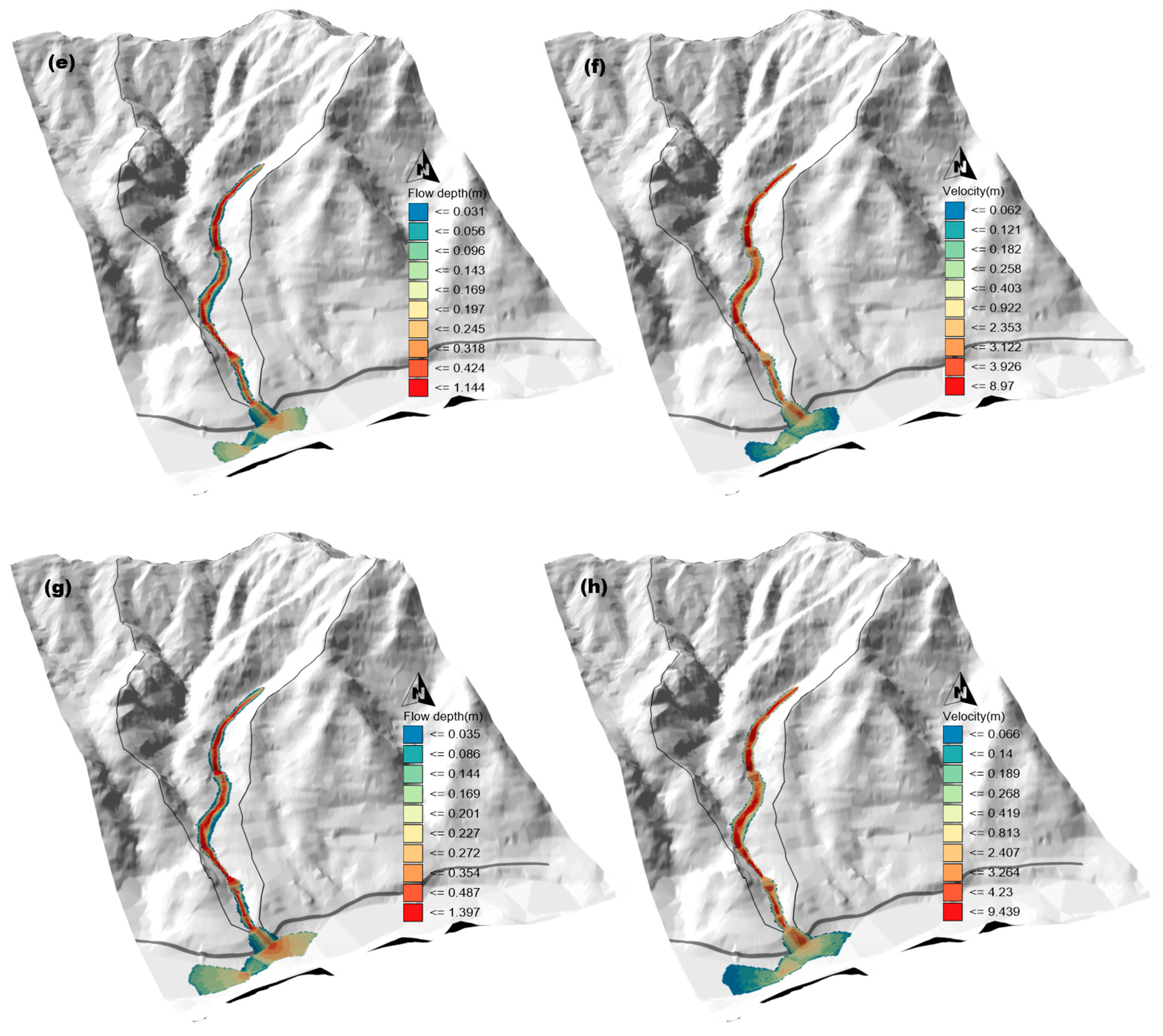
Debris flow events were simulated using the FLO-2D model, a numerical analysis tool for simulating debris flows. The debris flow disaster that occurred in the upper region of Jangsu Bridge 5 in Mt. Seorak exhibited a classic debris flow pattern: sediments rapidly moved from the initiation point down to transportation due to the steep terrain, spreading to both sides during deposition and converging into the river. For the simulation, different rainfall scenarios were considered, including the actual rainfall on the day of the debris flow incident, as well as probability-based rainfalls with return periods of 30, 50, and 100 years. These scenarios were utilized to simulate four distinct cases. The spatial resolution of the digital map DEM data was set at 5 m × 5 m for the topographical information. Figure 8 illustrates the primary outcomes from the four simulation cases, capturing variations in flow rates. These differences are reflected in key aspects of the debris flow process, such as flow depth, velocity, and diffusion area. Specifically, in case I (a) and (b), utilizing actual rainfall data, flow depths ranged from 0.041 to 8.254 m/s with flow velocities ranging from 0.037 to 0.861 m. The diffusion area of the debris flow basin was calculated by determining the last flow depth at which debris movement ceased.
Table 5 presents the outcome of the comparative analysis for each simulation. Flow depth, velocity, and diffusion area exhibited a gradual increase in response to the variation in flow rates. The average flow depth, calculated by determining the mean flow depth across all points influenced by the debris flow movement, ranged from a relatively low 0.192 to 0.237 m. This mean value was computed even for areas with comparably shallow flow depths, including sediment. The mean flow depth was calculated to be low due to the nature of the basin, which spreads widely in narrow valleys and sediments. When considering the flow depth during both the initiation and transportation phases of the debris flow, it is likely that this value would closely resemble the maximum flow depth.
For velocity, both the debris flow initiation zone and the transportation section exhibited higher calculated values. Nevertheless, the mean velocity was evaluated as relatively low, ranging from 1.057 to 1.492 m/s, due to the extensive sedimentary area. In the context of the final scenario, Case IV, the analysis indicated a maximum flow depth of 1.397 m, a velocity of 9.439 m/s, and a diffusion area spanning 40,725 m2.
In the simulation, the intensity of the debris flow is categorized by both flow depth and velocity. The flow depth is represented as h (m), while the flow velocity is denoted as v (m/s). The debris flow’s intensity index is the product of the maximum cumulative depth (h) and the maximum flow velocity (v), resulting in hv. This index is used to assess the severity of the debris flow. The risk associated with debris flow disaster is classified into three categories: high, medium, and low, as outlined in Table 6. This classification is determined through simulation. The disaster risk map provides the level and criteria for landslide hazard based on Swiss and Austrian standards [24].
The hazard susceptibility analyzed via the simulations was overlaid with aerial photographs taken at the time of the debris flow event. Figure 9a shows the overlap between debris flow hazard susceptibility and aerial photographs. Due to geographical features such as steep slopes and narrow valleys, most of the flow had a high hazard level from initiation to transport. In (b), the aerial photograph shows the destruction of roads during the debris flow event, while (c) indicates a high hazard level for roads in the debris flow hazard susceptibility.

4. Conclusions

This study utilized LiDAR surveys and FLO-2D numerical simulations to comprehensively assess the risk of debris flow damage in select watersheds of Seoraksan National Park, located in Hangye-ri, Inje-gun, Gangwon-do. LiDAR survey data can be utilized to accurately calculate the extent of debris flow diffusion and serve as a criterion for assessing the accuracy of FLO-2D simulation results. The primary conclusions of this study are as follows:
(1)
Employing on-site monitoring and terrestrial LiDAR technology, the actual extent of debris flow was meticulously scanned, resulting in the creation of high-resolution DEM spatial data. These data facilitated the calculation and analysis of the deposition and diffusion areas downstream from the debris flow generation zone, estimating it to be approximately 21,300 square meters.
(2)
Debris flow phenomena were replicated using the FLO-2D model. The simulation incorporated actual rainfall data from the event and probabilistic rainfall patterns associated with return periods of 30, 50, and 100 years. The simulation using actual rainfall revealed a maximum flow depth of 0.86 m, a peak velocity of 8.254 m per second, and a diffusion area of around 20,900 square meters. This closely aligned with the findings of the LiDAR survey, which indicated a value of 21,300 square meters. In the case of the 100-year frequency, the maximum flow depth increased to 1.397 m, the peak velocity surged to 9.439 m per second, and the diffusion area expanded to 40,725 square meters. Across simulations, it was observed that flow depth, velocity, and diffusion area exhibited gradual increments in response to varying flow rates.
(3)
Risk assessment was conducted by overlapping the debris flow disaster map with an aerial photograph captured during the disaster. The debris flow intensity index (hv) was extracted for Jangsu Bridge 5 (National Highway 44), leading to the creation of a disaster risk map. This analysis indicated a high risk of debris flow disaster for the majority of the debris flow generation zone and the flow path towards transportation. In the downstream region, actual debris flow encroached upon the road and entered the river, yielding a high level of risk.
This study holds the potential to serve as foundational data for mitigating damage to infrastructure and residences. Moreover, it can aid in the selection of suitable sites for runoff reduction facilities to enhance safety in regions susceptible to mountain slope instability and debris flow induced by heavy rainfall events.

Author Contributions

Performed database construction and analysis and wrote the manuscript, C.O.; oversaw the results of the analysis and revised the manuscript, K.J. All authors have read and agreed to the published version of the manuscript.

Funding

This work was supported by the National Research Foundation of Korea (NRF) grant funded by the Korea government (MSIT) (No. NRF-2021R1A2C1008568).

Data Availability Statement

The data supporting the results of this study are available from the author upon reasonable request.

Conflicts of Interest

The authors declare no conflict of interest.

References

  1. Sidel, R.C.; Ziegler, A.D.; Negishi, J.N.; Nik, A.R.; Siew, R.; Turkelboom, F. Erosion Processes in Steep Terrain-Truths, Myths, and Uncertainties Related to Forest Management in Southeast Asia. For. Ecol. Manag. 2006, 224, 199–225. [Google Scholar] [CrossRef]
  2. Wang, N.S.; Yi, R.H.; Liu, D. A solution method to the problem proposed by Wang in voting systems. J. Comput. Appl. Math. 2008, 221, 106–113. [Google Scholar] [CrossRef]
  3. O’Brien, J.S.; Julien, P.Y. Laboratory analysis of mud flow properties. J. Hydraul. Eng. 1988, 8, 877–887. [Google Scholar] [CrossRef]
  4. O’Brien, J.S.; Julien, P.Y.; Fullerton, W.T. Twodimensional water flood and mudflow simulation. J. Hydraul. Eng. 1993, 119, 244–261. [Google Scholar] [CrossRef]
  5. Iverson, R.M.; Ried, M.E.; LaHusen, R.G. Debris flow mobilization from landslides. Annu. Rev. Earth Planet. Sci. 1997, 25, 85–138. [Google Scholar] [CrossRef]
  6. Imran, J.; Harff, P.; Parker, G. A numerical model of submarine debris flow with graphical user interface. Comput. Geosci. 2001, 27, 717–729. [Google Scholar] [CrossRef]
  7. Takahashi, T.; Tsujimoto, H. Mechanics of granular flow in inclined chute. J. Hydraul. Coast. Environ. Eng. JSCE 1984, 565, 57–71. [Google Scholar] [CrossRef] [PubMed]
  8. Kim, K.S. Characteristics of Basin topography and Rainfall Triggering Debris Flow. J. Civ. Environ. Eng. Res. KSCE 2008, 28, 236–271. [Google Scholar]
  9. Fan, L.; Lehmann, P.; McArdell, B.; Or, D. Linking rainfall-induced landslides with debris flows runout patterns towards catchment scale hazard assessment. Geomorphology 2017, 280, 1–15. [Google Scholar] [CrossRef]
  10. Mark, T.J.; Van Westen, C.J. Deterministic Modelling in GIS-Based Landslide Hazard Assessment. In Geographical Information Systems in Assessing Natural Hazards; Springer: Dordrecht, The Netherlands, 1995; pp. 57–77. [Google Scholar]
  11. Lin, J.Y.; Yang, M.D.; Lin, B.R.; Lin, P.S. Risk assessment of debris flows in Songhe Stream, Taiwan. Eng. Geol. 2011, 123, 100–112. [Google Scholar] [CrossRef]
  12. Choi, J.H. Analysis of Debris Flow of Chun-chon Landslide Area using Numerical Methods. J. Eng. Geol. 2017, 27, 59–66. [Google Scholar]
  13. Lo, C.M.; Feng, Z.Y.; Chang, K.T. Landslide hazard zoning based on numerical simulation and hazard assessment. Geomat. Nat. Hazards Risk 2018, 9, 368–388. [Google Scholar] [CrossRef]
  14. An, H.; Ouyang, C.; Wang, F.; Xu, Q.; Wang, D.; Yang, W.; Fan, T. Comprehensive analysis and numerical simulation of a large debris flow in the Meilong catchment, China. Eng. Geol. 2022, 298, 106546. [Google Scholar] [CrossRef]
  15. Kim, Y.J.; Kim, T.W.; Kim, D.K.; Yoon, J.S. Debris flow characteristics and sabo dam function in urban steep slopes. J. Korea Water Resour. Assoc. KWRA 2020, 53, 627–636. [Google Scholar]
  16. Zhang, T.; Yin, Y.; Li, B.; Liu, X.; Wang, M.; Gao, Y.; Wan, J.; Gnyawali, K.R. Characteristics and dynamic analysis of the February 2021 long-runout disaster chain triggered by massive rock and ice avalanche at Chamoli, Indian Himalaya. J. Rock Mech. Geotech. Eng. 2023, 15, 296–308. [Google Scholar] [CrossRef]
  17. Ji, J.; Zhang, C.; Gao, Y.; Kodikara, J. Reliability-based design for geotechnical engineering: An inverse FORM approach for practice. Comput. Geotech. 2019, 111, 22–29. [Google Scholar] [CrossRef]
  18. Ji, J.; Wang, C.W.; Gao, Y.; Zhang, L. Probabilistic investigation of the seismic displacement of earth slopes under stochastic ground motion: A rotational sliding block analysis. Can. Geotech. J. 2020, 58, 952–968. [Google Scholar] [CrossRef]
  19. Ji, J.; Cui, H.; Zhang, T.; Song, J.; Gao, Y. A GIS-based tool for probabilistic physical modelling and prediction of landslides: GIS-FORM landslide susceptibility analysis in seismic areas. Landslides 2022, 19, 2213–2231. [Google Scholar] [CrossRef]
  20. Liu, Q.; Huang, D.; Huang, Z.; Zhang, B.; Xu, X. Total probababilistic measure for the potential risk of regional roads exposed to landslides. Reliab. Eng. Syst. Saf. 2022, 228, 108822. [Google Scholar] [CrossRef]
  21. Tang, Y.; Guo, Z.; Wu, L.; Hong, B.; Feng, W.; Su, X.; Li, Z.; Zhu, Y. Assessing Debris Flow Risk at a Catchment Scale for an Economic Decision Based on the LiDAR DEM and Numerical Simulation. Front. Earth Sci. 2022, 10, 1–21. [Google Scholar] [CrossRef]
  22. Ministry of Public Safety and Security. Development of Precision Hazard Risk Assessment Methods and Hazard Maps for Landslides and Debris Flows Due to Heavy Rainstorms; MPSS: Sejong, Republic of Korea, 2015. [Google Scholar]
  23. O’Brien, J.S. FLO-2D User Manual. FLO-2D Software, Inc.: Nutrioso, AZ, USA, 2018. [Google Scholar]
  24. Fiebiger, G. Hazard mapping in Austria. J. Torrent Avalanche Landslide Rockfall Eng. 1997, 134, 93–104. [Google Scholar]
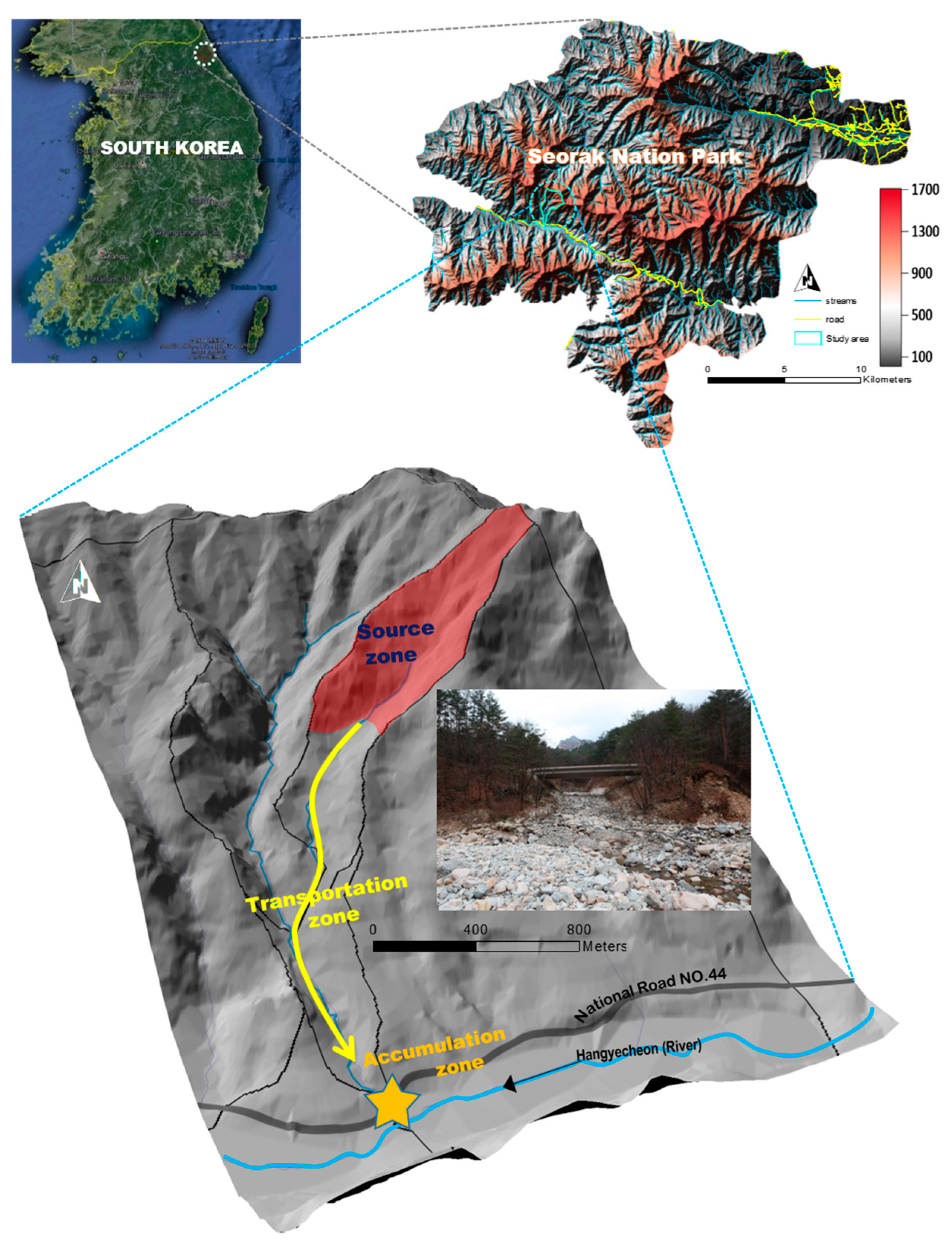
Figure 1. Location of the selected study area (Seorak national park near Jangsu bridge 5).
Water 15 03454 g001
Figure 2. Photographs of debris flow-induced damage (erosion and sediment section).
Water 15 03454 g002
Figure 3. Hydrograph and accumulated rainfall: (a) Daily rainfall and accumulative rainfall, (b) hourly rain fall and accumulative rainfall.
Water 15 03454 g003
Figure 4. LiDAR measuring equipment and point cloud data: (a) LiDAR measuring equipment, (b) point cloud data before filtering, (c) point cloud data after filtering.
Water 15 03454 g004
Figure 5. Spatial database of the target watershed: (a) DEM map, (b) slope map, (c) soil map, (d) geological map.
Water 15 03454 g005
Figure 6. Concept of field survey and terrestrial LiDAR measurement. (a) Debris flow Initiation zone, (b) Flow zone, (c) Deposition zone.
Water 15 03454 g006
Figure 7. Comparison of aerial imaging and LiDAR measurement DEM: (a) Seorak Mt. aerial photograph, (b) LiDAR DEM.
Water 15 03454 g007
Figure 8. Comparison of FLO-2D simulation results for debris flow occurrence area according to flow rate values of cases I, II, III, and IV: Case I (debris flow occurrence rainfall data): (a) Flow depth, (b) velocity. Case II (30-year frequency): (c) Flow depth, (d) velocity. Case III (50-year frequency): (e) flow depth, (f) velocity. Case IV (100-year frequency): (g) flow depth, (h) velocity.
Water 15 03454 g008aWater 15 03454 g008b
Figure 9. Hazard map based on Jangsu bridge 5 (national road no.44) (a) Overlap between debris flow hazard susceptibility and aerial photographs; (b) the aerial photograph shows the destruction of roads during the debris flow event; (c) the debris flow hazard vulnerability of the road.
Water 15 03454 g009
Table 1. Probable rainfall intensity for Inje-gun (mm).
Return Period of Rainfall (mm)
DurationEvent Rainfall of
Debris Flow
30 Year50 Year100 Year
60 min49.561.866.973.7
Table 2. Empirical coefficients of yield stress and dynamic viscosity.
Source τ y = α 1 e β 1 C v (Dynes/ c m 2 ) η = α 2 e β 2 C v (Poises)
α 1 β 1 α 2 β 2
Aspen Pit 10.18125.70.036022.1
Aspen Pit 22.7210.40.053814.5
Aspen Natural Soil0.15218.70.0013628.4
Aspen Mine Fill0.047321.10.12812.0
Aspen Watershed0.038319.60.00049527.1
Aspen Mine Source Area0.29114.30.00020133.1
Glenwood 10.034520.10.0028323.0
Glenwood 20.076516.90.06486.20
Glenwood 30.00070729.80.00063219.9
Glenwood 40.0017229.50.00060233.1
Note: Data from (O’Brien & Julien, 1988) [2].
Table 3. Resistance parameter for laminar flow.
SurfaceRange of K
Concrete/asphalt24–108
Bare sand30–120
Graded surface90–400
Bare clay–loam soil, eroded100–500
Sparse vegetation1000–4000
Short prairie grass3000–10,000
Bluegrass sod7000–50,000
Note: Data form (FLO-2D User manual 2018) [23].
Table 4. Input parameters of FLO-2D simulation.
Manning
Coefficient (n)
Viscosity vs. Sediment Concentration Yield Stress vs. Sediment ConcentrationLaminar Flow
Resistance (K)
Forestαβαβ500
0.020.038319.60.00049527.1
Table 5. FLO-2D simulation results.
Maximum Flow
Depth (m)
Mean Flow
Depth (m)
Maximum Flow
Velocity (m/s)
Mean Flow
Velocity (m/s)
Diffusion Area (m2)
Case I0.8610.1928.2541.05720,900
Case II1.0400.1998.8001.42329,450
Case III1.1440.2028.9701.44235,625
Case IV1.3970.2379.4391.49240,725
Table 6. Hazard classification based on debris flow intensity.
Debris Flow
Risk
Maximum Simulated
Accumulation Depth h (m)
RelationMaximum Simulated Accumulation
Depth and Velocity vh (m2/s)
Highh >1.0 mORvh > 1.0 m2/s
Medium0.2 m < h < 1.0 mAND0.2 m < vh < 1.0 m2/s
Low0.2 m < h < 1.0 mANDvh < 0.2 m2/s
Note: Data from (FLO-2D User manual 2018) [23].
Disclaimer/Publisher’s Note: The statements, opinions and data contained in all publications are solely those of the individual author(s) and contributor(s) and not of MDPI and/or the editor(s). MDPI and/or the editor(s) disclaim responsibility for any injury to people or property resulting from any ideas, methods, instructions or products referred to in the content.