Monitoring Discharge in Vegetated Floodplains: A Case Study of the Piave River

Abstract

The accurate assessment of discharge in vegetated floodplains during floods is a persistent challenge in river engineering due to the difficulty of acquiring hydraulic data, the variability in vegetation roughness, and the limitations of on-site vegetation characterization. This study introduces a novel approach that combines the continuous slope-area method with LiDAR-derived vegetation data and water depths measured with piezoresistive sensors to evaluate floodplain discharges while considering variations in roughness coefficients induced by arboreal vegetation. We apply this approach to a specific reach of the Piave River in Italy using data collected during the December 2020 flood event. The study demonstrates the capability of the employed measurement system to record extreme floods and emphasizes the importance of including vegetation roughness variations in floodplain discharge calculations. The proposed approach has the potential to be applied in similar scenarios, providing valuable insights for floodplain discharge estimation in vegetated areas.

1. Introduction

Floodplains are complex and dynamic areas that play a crucial role in the functioning of riverine ecosystems. They serve as vital interfaces between terrestrial and aquatic environments, facilitating nutrient exchange and providing food and shelter for various species of animals and plants [1].

During floods, floodplains can act as pseudo-storage reservoirs, reducing and delaying peak flows downstream [2,3,4]. In vegetated floodplains, vegetation can partially obstruct the streamflow area, increasing water levels and reducing flow velocities as well as river conveyance capacity [5,6,7]. Reliable discharge prediction in vegetated floodplains is essential for effective ecosystem management and flood risk mitigation [8,9]. However, this is a challenging task given the complex vegetation–water interactions, the difficulty of collecting reliable field data for hydraulic models, and the inherent risks associated with direct discharge measurements during floods.

From a hydraulic standpoint, a quantity that can significantly influence the discharge capacity of the floodplain is vegetation roughness [5,10,11]. Extensive research has focused on estimating vegetation roughness [10,12,13], using methods ranging from flume experiments to analytical and numerical studies. Several analytical models have been proposed to assess roughness coefficients induced by vegetation [14,15,16,17,18,19]. A broad description of these models can be found in literature reviews like [10,20,21].

However, implementing some of these models on a river scale can be challenging [22], as acquiring vegetation parameters in the field is time-consuming and expensive. To overcome this issue, some recent studies [23,24] rely on remote sensing techniques to map and measure vegetation parameters such as canopy height, tree diameter, and vegetation density. These techniques offer new opportunities to improve roughness assessments on a large scale [25,26,27].

River engineers employ numerous approaches to estimate floodplain discharge, each with its own advantages and limitations. One of the most common approaches is to use 1D or 2D hydraulic models, assigning roughness coefficients based on literature values [28,29,30]. The roughness coefficient is then adjusted to minimize the difference between the hydraulic model predictions and field data, such as water levels [31]. Once the roughness value is calibrated, the hydraulic model can be employed to predict discharge. However, this approach is only feasible when instrumental records or historical flood data are available.

Another indirect discharge estimation technique is the slope-area method [32]. This method relies on the Manning equation and employs water depth measurements taken at multiple points along at least two cross-sections of the river [33]. The discharge is determined by calculating the water-surface slope from these measurements and using data from the cross-section and the roughness coefficient (see Section 3.3). This approach is particularly advantageous for rivers with relatively simple cross-sectional geometries and low gradient streams under uniform flow conditions [32]. However, it may exhibit poor performance in high-gradient streams, where measurement errors are often large and can lead to the overestimation of peak discharges [34]. To obtain accurate discharge predictions, the study reach must be long and free of significant changes in cross-sections, as well as bridges, bends, and other singularities, such as flow control structures, which can potentially lead to non-uniform flow conditions [34,35]. An extension of this method, known as the continuous slope-area (CSA) method, has been adapted for event hydrograph computation [36].

A third approach to floodplain discharge estimation involves indirect measurements using in situ devices, such as current meters and stage gauges, or direct measurements through Acoustic Doppler Current Profilers (ADCPs) [33]. In-situ devices are relatively inexpensive and easy to deploy, but they are exposed to the water current and can be easily damaged or lost under high-flow conditions [37]. ADCP devices have gained popularity due to their non-intrusive nature and can calculate discharge in real-time by traversing the watercourse from one bank to the other [38]. Nevertheless, data acquisition with ADCPs in floodplains can be affected by operational problems, such as limited accessibility [39], high current velocities, and the presence of vegetation and floating debris, which can restrict boat motion [33]. Moreover, since floods can occur unexpectedly, it is difficult to reach the site to perform the measurements on the same day the flood is taking place. All these factors can ultimately lead to reduced measurement quality and accuracy [40].

Novel remote sensing technologies have opened new avenues for discharge estimation, integrating satellite and in situ observations with approaches based on hydraulic laws (e.g., Manning equation), rating curves, or hydraulic modeling [41,42,43]. Among satellite sensors, both radar altimeters and optical sensors have emerged as significant contributors to discharge derivation [43]. For instance, radar altimetry sensors measure water levels of rivers and floodplains that exhibit good agreement with in situ measurements [44,45]. Optical sensors measure river extent or width and its variations, thanks to their frequent (some of them daily) observations and large spatial coverage [46,47]. Despite these advancements, challenges in this approach persist, including the roughness estimation [48] and the balance between the spatial and temporal resolution—a high spatial resolution entails fewer observations. Additionally, ground data remain necessary to establish rating curves that link satellite observations with in situ discharge data [49].

Estimating discharge in vegetated floodplains represents a complex task due to several inherent limitations. Dense vegetation, including trees, shrubs, and bushes, obstructs water flow and interferes with velocity measurements using instruments like ADCPs. Furthermore, vegetation exhibits significant variability within a floodplain, leading to fluctuations in roughness coefficients. Accessibility and safety concerns further compound these issues, especially during extreme floods. Additionally, gathering hydraulic and vegetation data in the field is usually demanding and complicated work.

To address some of these limitations, this study proposes an innovative approach for predicting floodplain discharges during flood events while considering the influence of arboreal vegetation on hydraulic roughness. This novel and integrated methodology combines the continuous slope-area method with on-site measurements of water depths and vegetation parameters acquired using a remote sensing technique. By implementing this comprehensive approach, we intend to provide valuable insights into discharge estimation within vegetated floodplains and address some of the complexities associated with field data collection and measurements.

This manuscript is organized as follows. Section 2 introduces the study area and outlines the approach used to characterize the vegetation in the field. Section 3 illustrates the water depth measurement system installed in the field, along with the methods employed to estimate the roughness coefficients for vegetation and riverbeds. Additionally, the slope-area method used for discharge calculation is explained. In Section 4, we apply the proposed methodology to analyze a flood event recorded using the measurement system, and we discuss the challenges encountered and insights gained from this experience. Finally, the conclusions of this study are drawn in Section 5.

2. Study Area

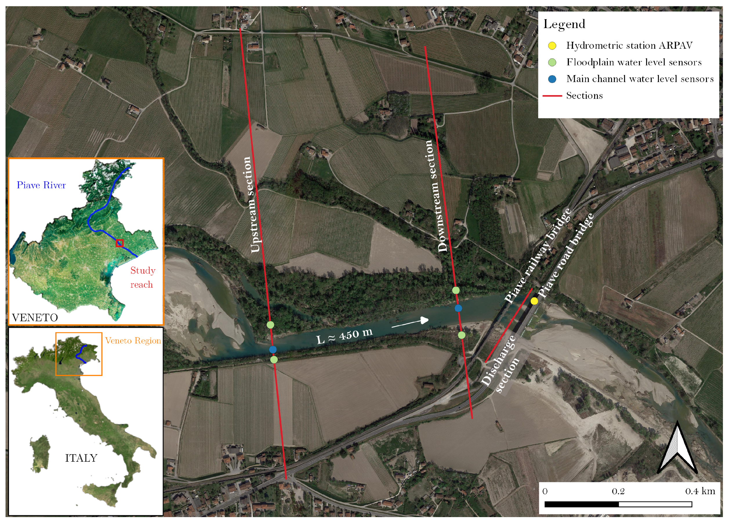
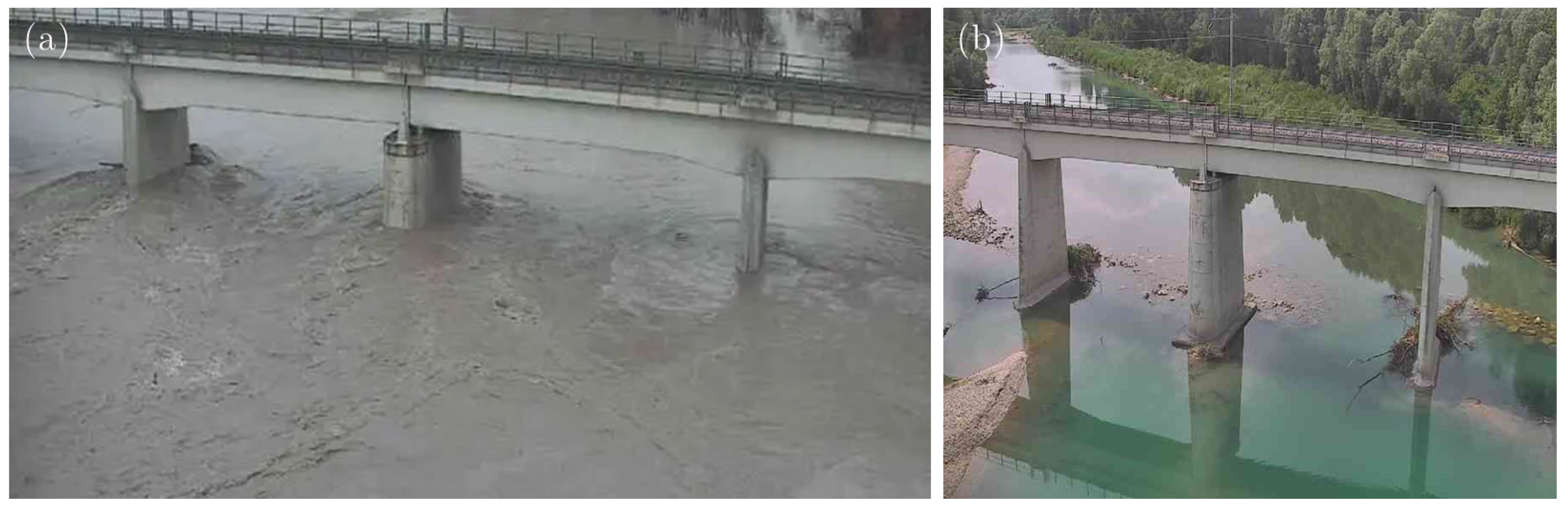
The Piave River is located in the Veneto region of northeastern Italy. The catchment area of the river is approximately 4130 km², and the main channel is around 220 km long. Here, we study a reach whose length is about 450 m and is located in the lower course of the basin, specifically upstream of the Piave railway bridge between the municipalities of Ponte di Piave and San Biagio di Callalta (Figure 1). The reach under study was selected due to its particular characteristics, which include (i) a significant presence of arboreal vegetation, (ii) a regular and rectilinear geometry, and (iii) the proximity to a hydrometric station operated by the Regional Agency for Environmental Prevention and Protection of Veneto (ARPAV), where water levels are measured.

The study area has predominantly flat terrain, rendering it highly susceptible to flooding. The river is about 60 m wide and has a mild slope of 0.1%. Mean temperatures range from 2 to 4 °C in winter and 33 to 35 °C in summer. The average annual precipitation in this area is between 800 and 1000 mm. June and November are the rainiest months, with an average precipitation of 90 to 100 mm [50].

The riparian and floodplain vegetation consists mainly of arboreal species, bushes, vineyards, and crops (see Figure 2). The riverbed is composed of fine materials such as sand and silts [51]. From a hydrological point of view, the river is subject to intra-annual streamflow variations due to anthropogenic actions (e.g., irrigation, agriculture, hydropower) and hydroclimatic fluctuations, which contribute to progressive morphological changes and higher peak flows [52].

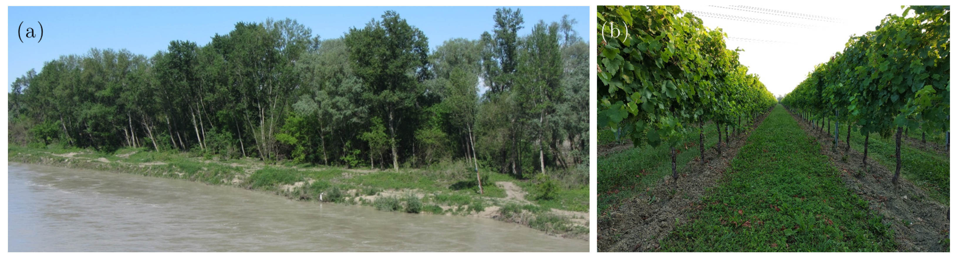
Characterization of Vegetation in the Field

The riverine vegetation in the study area is mainly a mosaic of forested and agricultural patches, including corn and vineyard fields (Figure 2). The left floodplain has a mix of forested and agricultural patches, while the right floodplain is predominantly characterized by agricultural land use (see Figure 1).

The forest stand parameters were derived from a field campaign conducted in 2020 and an analysis of high-density LiDAR data acquired in the spring of 2020 (more than 20 points/m²) coupled with a 10 cm resolution orthophotomosaic. Within the surveyed plots (radius = 10 m), the parameters recorded for live and dead trees include species, Diameter at Breast Height (DBH, i.e., measured at 1.3 m from the ground), and tree height. Such data were employed to derive the local wood volume. These values were then used both to train a classification algorithm to identify the predominant forest typologies from the available aerial images and to create specific linear models to spatialize the mean DBH and stand density (i.e., the mean number of trees per hectare), using the high-density LiDAR point clouds. This procedure allowed for the production of two raster maps with a cell size of 20 m × 20 m, representing a continuous prediction for the two target variables (i.e., tree density and mean DBH) across the whole riverine study area.

3. Materials and Methods

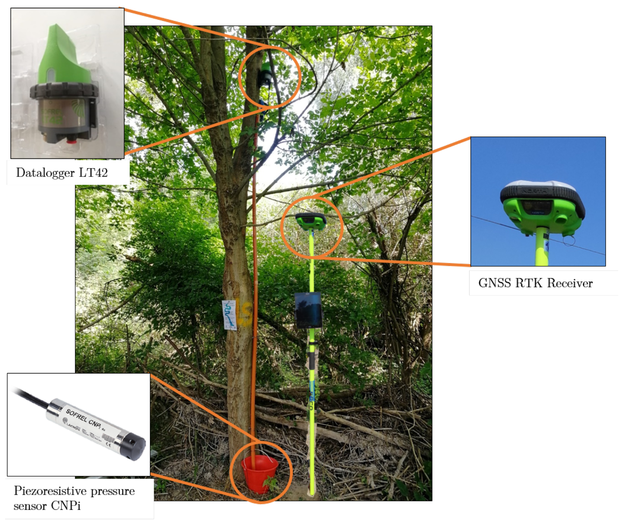
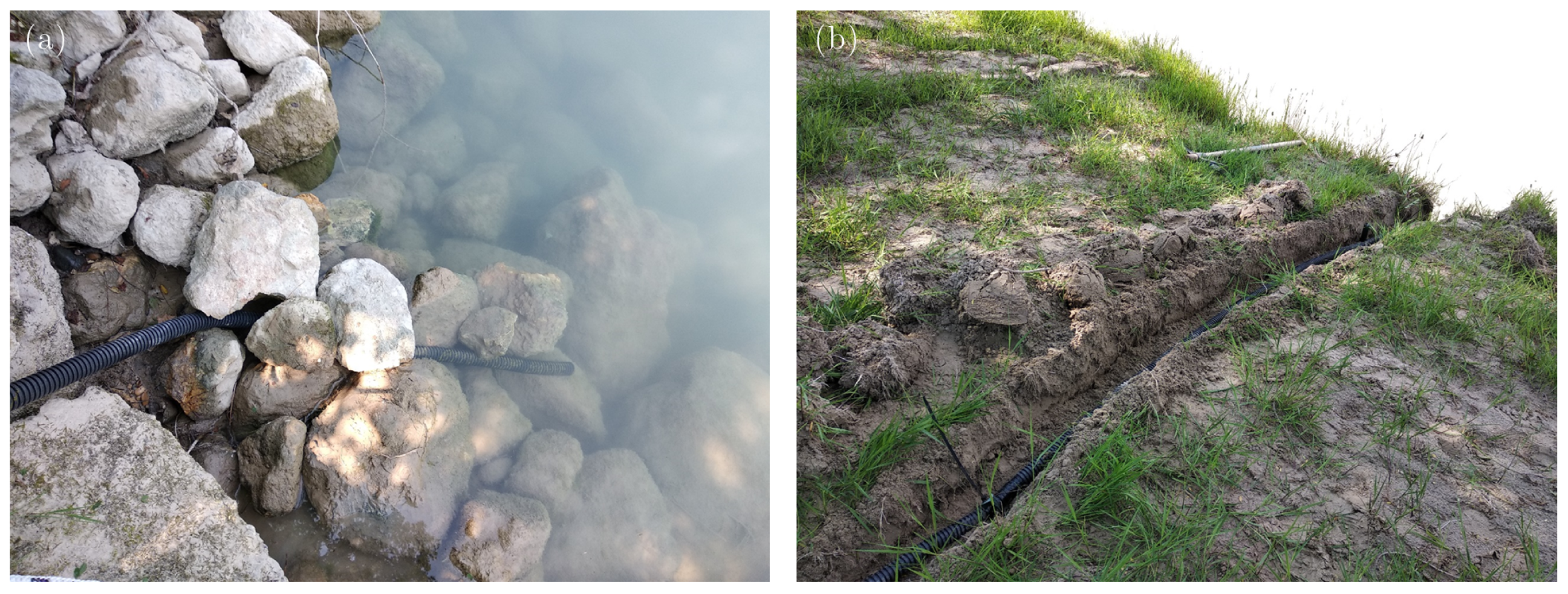
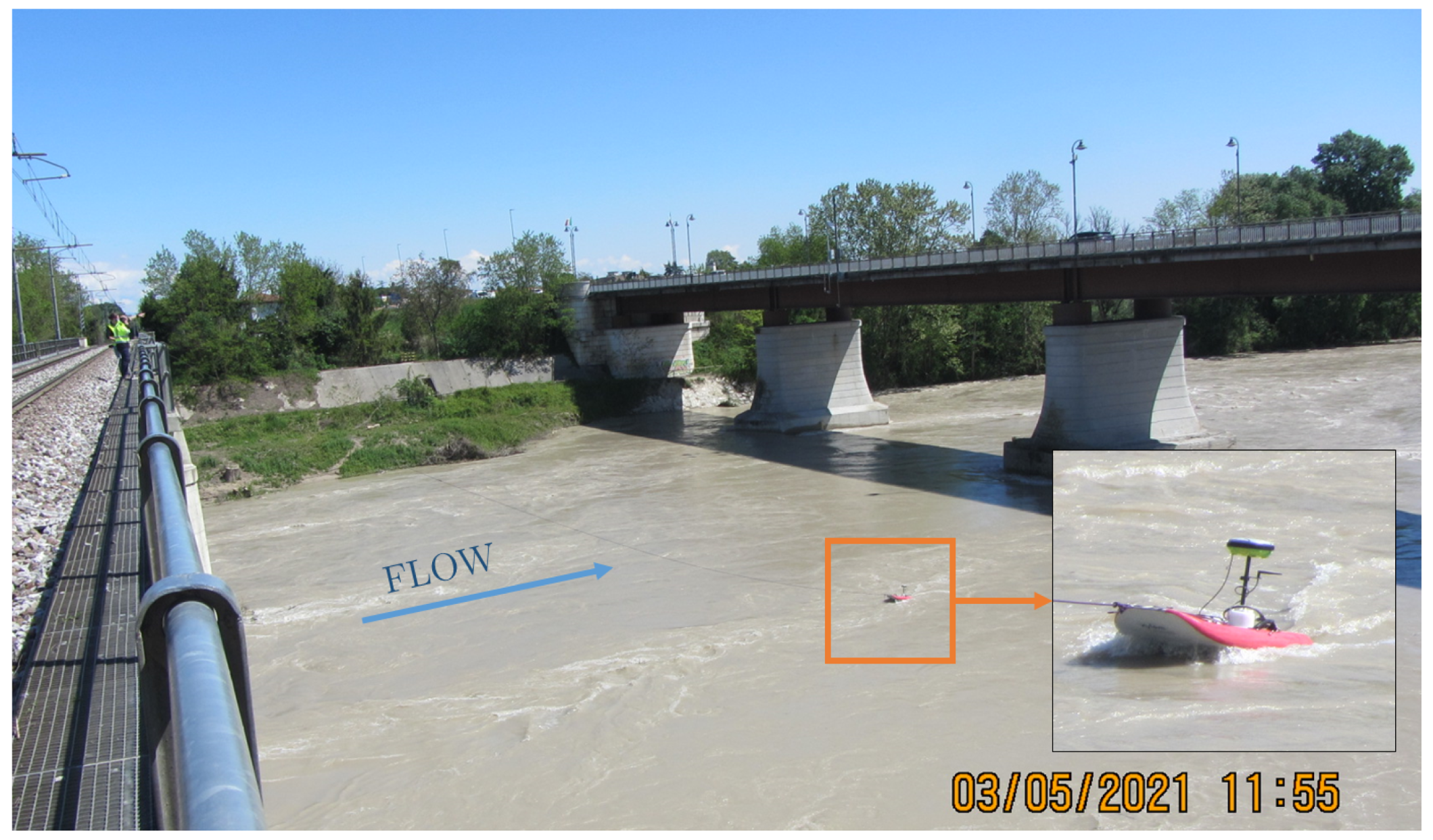
3.1. Field Measurement System

The purpose of the field measurement system is to quantify the water surface slope along the flow direction, which is going to be employed later in the application of the CSA method. This is performed by monitoring the variation in water levels of the riverbed and floodplains in six points of two cross-sections of the studied reach (Figure 1).

The selection of the instrumentation locations relied on data provided by the Eastern Alps District Authority, including water level records, cross-sectional surveys, land cover maps, and hydrological and hydraulic analysis reports. Using water level records, we identified flood-prone areas with frequently elevated water levels during flood events; cross-sectional surveys provided information about the topography of the zone, helping us recognize floodplains susceptible to substantial water accumulation and sections where non-zero water surface slopes can be measured; land cover maps aided in individuating sites rich in vegetation; and the hydrological and hydraulic reports were essential for understanding flood characteristics and the flow dynamics of the river during such events. Additionally, we conducted field inspections to determine the optimal specific locations for the instrumentation and define suitable materials and installation set-ups. This task was particularly challenging due to the absence of fixed structures capable of withstanding the force of water during flood events.

Given the mild slopes of the terrain, the prevalent agricultural and forest patches, and the lack of fixed and elevated structures favorable to placing more sophisticated instruments (such as radar, ultrasound sensors, or cameras) within the study area, we decided to use CNPi submersible piezoresistive sensors manufactured by Lacroix Sofrel to measure water levels. These sensors are equipped with a stainless-steel membrane and measure the pressure difference between the water surface and the sensor position. This differential pressure is directly proportional to the water level above the sensor. CNPi sensors are able to measure water depths up to 10 m and can endure temperatures ranging from −10 °C to +70 °C without causing any deviations in the measurements [53].

Water surface elevations are calculated based on water levels measured by the CNPi sensors and the elevation of the sensor position, which is determined using a GPS. For this purpose, we employed the GNSS RTK receiver produced by NORTH (see Figure 3). This versatile receiver is adaptable for different applications due to its operating system, which can interface with any software [54]. Data collection is carried out via a Bluetooth connection between the receiver and a smartphone through an application specially designed to record points and tracks using external GNSS receivers. An example of this type of application is SW Maps.

CNPi data are acquired and transmitted by connecting the sensor cable to another device, known as a data logger. In our setup, we employed the Lacroix data logger LT42, which is powered by an internal lithium battery. This device is capable of storing data locally and transmitting it to a remote server, allowing for real-time monitoring of instruments and data retrieval from any location. The design of the data logger LT42 is optimized to endure submersion in water up to a depth of 1 m for 100 days. This feature proves beneficial, especially in scenarios where floodwaters may exceed the elevation of the data logger.

For the experimental setup, the acquired instruments were six CNPi piezoresistive sensors and four data loggers LT42 from Lacroix Sofrel (see Figure 1 and Figure 3), which have proven to be reliable and efficient for our measurement needs.

Instrument installation at the experimental site was carried out in July 2020. Sensors within the floodplains were inserted inside rigid PVC pipes with a diameter of 40 mm. These pipes were anchored to trees to protect and fix the sensors, as shown in Figure 3. Moreover, a water bucket was employed to ensure continuous submersion of the sensor membrane, thereby preventing any potential deviations in the level measurements.

The sensors placed at the main channel are inside 40 mm diameter corrugated tubes. Due to the lack of stable structures near the riverbed, ensuring a fixed position for these sensors was a complex task. In the upstream section, the tube housing the sensors had to be surrounded by rocks in the riverbank (Figure 4a) to provide a stable setting. Otherwise, in the downstream section, the tube was buried along the riverbank until it reached the riverbed (Figure 4b).

Concerning the data loggers, they were positioned and firmly anchored to the trees at a height of 2 to 4 m above the land surface to provide stable and reliable data acquisition throughout the monitoring period. Each data logger can connect with up to two water level sensors. Consequently, the data loggers located on the right floodplain of the upstream section and the left floodplain downstream were linked to two sensors each: one for the floodplain and the other for the main channel. The two remaining sensors were connected to individual data loggers.

3.2. Hydraulic Roughness Estimation

3.2.1. Floodplain Vegetation Roughness

According to the literature studies [18,21,55], emergent rigid vegetation, such as non-submerged trees, significantly increases hydraulic roughness as water depth increases. Considering this, our study incorporates three well-known roughness models (Huthoff et al. [16], Baptist et al. [17], Luhar and Nepf [18]) to estimate the roughness coefficients for the arboreal vegetation within the study reach.

To implement the slope-area method, Equations (1)–(6) are employed to define the roughness for the arboreal vegetation, while for cultivated areas, we adopted a Manning coefficient value n = 0.050 s/${\mathrm{m}}^{1/3}$ obtained from the literature [30,56].

Huthoff et al. [16] propose a two-layer model that distinguishes between vegetated and non-vegetated parts and provides a formulation to estimate the depth-averaged velocity, which reads

$$V=\sqrt{\frac{2gJ}{C_{D}mD}}\left[\sqrt{\frac{h_v}{h}}+\frac{h-h_v}{h}{\left(\frac{h-h_v}{s}\right)}^{\frac{2}{3}\left(1-{\left(\frac{h}{h_v}\right)}^{-5}\right)}\right]$$

(1)

where V is depth-averaged velocity, g is gravity acceleration, J is total energy slope, $C_D$ is the drag coefficient, m is number of stems per surface area, D is mean vegetation diameter, $h_v$ is mean vegetation height, h is water depth, and $s=1/\sqrt{m}-D$ is the average distance between vegetation.

Subsequently, the roughness coefficient can be determined with the Manning equation and the computed depth-averaged velocity.

Baptist et al. [17] derived an equation to determine the Chézy coefficient (C) through an analytical solution for the horizontal momentum equilibrium.

$$C=\sqrt{\frac{1}{1/C_b^2+\left(C_{D}mD{h}_v\right)/\left(2g\right)}}$$

(2)

where $C_b$ is the Chézy roughness coefficient for bare soil.

The roughness coefficients, Manning (n) and Chézy (C), are related as [57]:

$$\frac{n\sqrt{g}}{R^{1/6}}=\frac{\sqrt{g}}{C}$$

(3)

where R is the hydraulic radius.

According to Luhar and Nepf [18], the total flow resistance mainly depends on the blockage factor $\left(B_x\right)$, which is the channel portion obstructed by the vegetation, and it is determined by:

$$B_x=\frac{w{h}_v}{hB}$$

(4)

where w is the vegetation width and B the channel width. The following equations describe the relationship between $B_x$ and the Manning coefficient:

$$n\left(\frac{\sqrt{g}}{K{h}^{1/6}}\right)={\left(\frac{C_{D}ah}{2}\right)}^{1/2}{B}_x=1$$

(5)

$$n\left(\frac{\sqrt{g}}{K{h}^{1/6}}\right)={\left(\frac{C_{*}}{2}\right)}^{1/2}{\left(1-B_x\right)}^{-3/2}{B}_x<1$$

(6)

where $K=1$ m${}^{1/3}$s${}^{-1}$ is a constant that makes the equation dimensionally correct, a is the frontal area of vegetation per unit volume, and $C_{*}=0.05-0.13$.

Vegetation roughness coefficients are evaluated for each flow depth recorded during the flood using the diameters, densities, and heights of the trees in the study area, which were estimated as explained in Section 2.

3.2.2. Riverbed Roughness

The riverbed material at the examined reach mainly consists of fine sand and coarse silt, as indicated by a granulometry study performed with a Pario Automated Particles Size Analysis instrument manufactured by METER [58] on four riverbed samples collected in July 2020. The Manning coefficient was manually calibrated in a one-dimensional (1D) hydraulic model using the HEC-RAS software version 5.0.7 [59]. The water level and discharge data gathered during a measurement campaign held in May 2021 were used to determine the Manning coefficient that aligns this data with the values obtained from the hydraulic model.

On 3 May 2021, we conducted discharge measurements of the Piave river, using the River Surveyor M9, an ADCP instrument from Sontek. To perform the measurement, the ADCP is mounted on a vessel that moves along a river cross-section (Figure 5). The ADCP measures water velocity at various depths within the water column by emitting acoustic signals in 3 or 4 directions at specific angles relative to the vertical axis. These signals bounce off the riverbed or suspended water particles, and the frequency shift between successive echo signals corresponds to the relative velocity between the ADCP and the particles responsible for the signal reflection. After subtracting the velocity component of the instrument, the ADCP measures water velocity in three directions. To calculate discharge, the velocities acquired at multiple points of the cross-section are multiplied by the corresponding point areas [38,60]. In addition to flow velocities and discharges, ADCP devices can also provide bathymetry data.

The precise measurement site is an intermediate section between the Piave railway and road bridges (Figure 1). A precipitation event that took place on 2 May 2021, resulted in elevated water levels that filled the main channel but did not reach the vegetated floodplains. Therefore, the event provides an opportune scenario for estimating the roughness coefficient of the riverbed. Figure 5 shows a photograph taken from the railway bridge during the flow measurement campaign.

Table 1. Discharge, width, velocity, flow area, and water surface elevation measurements (WSE) conducted on 3 May 2021.

Transect	Q [m${}^3$/s]	B [m]	V [m/s]	A [m2]	WSE [m.a.s.l]	WSE ARPAV 1 [m.a.s.l]
1	255.17	127.13	1.17	217.81	3.72	3.62
2	261.45	131.78	1.65	158.69	3.74	3.59
3	261.24	126.39	1.30	200.86	3.73	3.59
4	259.43	125.62	1.68	154.06	3.73	3.59
5	254.28	123.50	1.39	183.27	3.73	3.59
6	257.03	128.63	1.68	153.32	3.74	3.59
Average	258.10	127.18	1.48	178	3.73	3.60

Notes: ¹ Data acquired from ARPAV website for the Ponte di Piave Hydrometric station [61]. Q: water discharge, B: section width, V: mean flow velocity, A: flow area, and WSE: water surface elevation.

summarizes the hydraulic parameters estimated from the measurements performed with the ADCP. In this context, a measurement, also referred to as a transect, means traversing the cross-section of the river from one bank to the other. For a reliable discharge estimation, it is recommended to gather at least four transects, all of which should be within 5% of the mean discharge [38]. In our study, a total of six transects were acquired, and their average value was employed for calibrating the Manning coefficient within the 1D model.

For cross-validation, we undertook a comparison between the water surface elevations (WSE) acquired through the ADCP and those registered by the hydrometric sensor placed by ARPAV in the Piave road bridge section. The discrepancies between the ADCP and ARPAV values range from 10 to 15 cm. These differences can be primarily attributed to the distinct measurement techniques. The ARPAV sensor captures data at a specific localized point, whereas the ADCP estimates the water surface elevations along the entire cross-section. The value provided in the table (and used for comparisons) is an average of these values, which range from 3.63 to 3.83 along the cross-section.

The 1D hydraulic model was based on cross-sectional data provided by the Eastern Alps District Authority and the discharge cross-section surveyed by the ADCP. By adjusting the Manning coefficient associated with the main channel within the 1D model, we found that a value of n = 0.0268 s/m${}^{1/3}$ accurately reproduced the water level, discharge, and hydraulic quantities obtained in the measurement section. This Manning coefficient value is consistent with values previously reported in the literature for similar riverbed materials [62,63]. According to the HEC-RAS model, for a discharge of Q = 258 m³/s, the WSE is 3.73 m.a.s.l.

3.3. Slope-Area Method

The slope-area method relies on Manning’s equation and is typically employed to estimate the peak flow of a hydrograph [32]. The continuous slope-area (CSA) method, on the other hand, allows for the estimation of a complete-event discharge hydrograph [36,64]. The CSA method uses continuous hydrometric level data measured at the two endpoints of a reach, an upstream and a downstream point.

The method is implemented as follows:

• Conveyance of upstream ($K_u$) and downstream ($K_d$) sections are estimated as:

  $$K_i=\left(\frac{1}{n}\right)A_i{R}_i^{2/3}\to i=u,d$$

  (7)

  where n is the Manning coefficient of the reach under analysis, $A_i$ is the wetted area of the i-th cross-section, and $R_i$ is the hydraulic radius of the i-th cross-section. Hydraulic radius is defined as the ratio between the wetted area and the wetted perimeter.
• Compute the mean conveyance of the slope-area reach (K) as the geometric mean of the conveyance of the upstream and downstream cross-sections, i.e., $K={\left(K_u{K}_d\right)}^{1/2}$.
• Estimate a first approximation of the friction slope, S, as:

  $$S=\frac{F}{L}$$

  (8)

  where $F=h_u-h_d$, i.e., the difference of the water surface elevation measured at the upstream and the downstream cross-sections, and L is the flow length between such sections.
• Estimate a first approximation of discharge, Q, as:

  $$Q=K{S}^{1/2}$$

  (9)
• Compute velocity head at the upstream and downstream cross-sections, $h_{v,i}$, as:

  $$h_{v,i}=\frac{\alpha {\left(\frac{Q}{A_i}\right)}^2}{2g}$$

  (10)

  where $\alpha$ is the velocity-head coefficient, which we consider equal to 1.
• Compute a second approximation of the friction slope, $S^{\prime }$:

  $$S^{\prime }=\frac{F+\left(h_{v,u}-h_{v,d}\right)}{L}$$

  (11)
• Compute a second approximation of discharge, $Q^{\prime }$:

  $$Q^{\prime }=K{S}^{\prime 1/2}$$

  (12)

The computations from 5 to 7 are repeated until the difference between Q and $Q^{\prime }$ reaches a previously established threshold value $\epsilon$.

4. Results

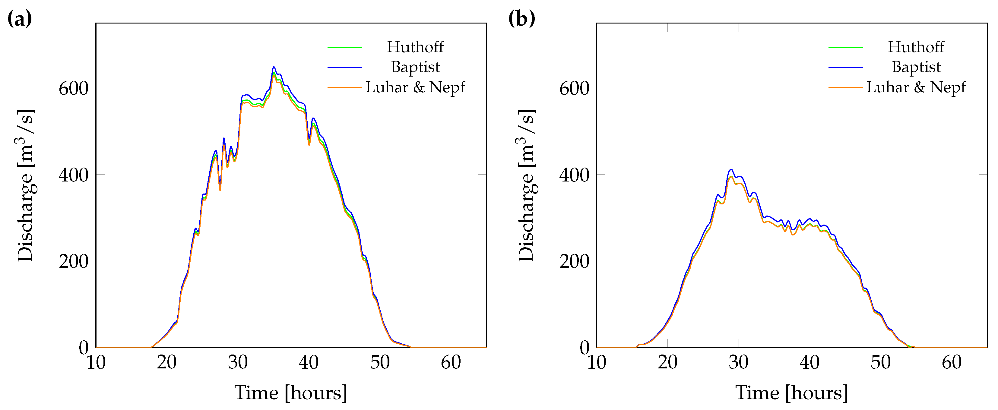
4.1. Discharge Estimation

Between December 5th and 7th, 2020, a significant flood event took place in the study area, providing an opportunity to activate the measurement system in the field.

The rainfall event occurred from the afternoon of December 4th to the evening of December 6th. During this period, the accumulated precipitation ranged between 200 and 500 mm in the surrounding area of the upper part of the river, and reached approximately 300 mm in the river basin, four times more than the expected monthly average of 84 mm, calculated based on data from 1994 and 2019 [65]. Strong winds prevailed, with peak gusts of approximately 140–150 km/h in mountainous regions and 80–100 km/h in foothill areas. Significant snow accumulations occurred, particularly at altitudes above 1200–1400 m, with depths of about 70–90 cm [66].

The accumulated rainfall resulted in a substantial increase in the water level, which exceeded 10 m.a.s.l., causing the flood to extend into the adjacent floodplains. Figure 6 shows contrasting images of the river during flood- and low flow conditions. These images were captured by a monitoring webcam at the Piave road bridge, installed by the Municipality of Ponte di Piave [67].

The measurement system recorded water levels during the flood in the upstream and downstream sections of the study reach, allowing us to use the CSA method to estimate discharge. Since water level sensors are installed in the two floodplains and the main channel, the idea is to compute discharges in three distinct areas: the left floodplain, the right floodplain, and the main channel, with the sum of these values equaling the total discharge.

Given the strong current, the sensors in the main channel were detached from their anchorage during the flood, rendering their measured data invalid. Thus, the analysis presented here is limited to the data collected by the sensors in the floodplains.

Figure 7 depicts the water surface elevation (WSE) during the flood, as measured by the floodplain sensors and the hydrometric station of ARPAV [61]. The sensors are located at different elevations, so they were activated at different times during the flood. The figure shows the data for the time window in which all sensors were operational, i.e., between hours 15 and 55 of the analysis period.

According to the graph, all WSE values of upstream and downstream sections are higher than those recorded at the ARPAV hydrometric station at the peak discharge (32 h). The WSE values of the floodplain sensors are, on average, 15 and 30 cm higher than the ARPAV sensor for downstream and upstream sections, respectively. The water level’s increment in the upstream direction of the river can be attributed to the development of a backwater profile generated when the flow encounters the restricted cross-section of the bridges and their supporting piles.

In particular, before the water surface elevation reaches 9.5 m.a.s.l., the WSE values in the left floodplain of the downstream section are lower than those in the right floodplain. One possible explanation for this is that the presence of arboreal vegetation on the left floodplain (Figure 1) impedes the water flow, decreasing the velocity. On the contrary, the absence of such vegetation in most parts of the right floodplain allows water to spread faster with higher velocities. Furthermore, as the floodplain area on the right side narrows toward the bridges, at the beginning of the flood, water accumulation becomes more pronounced, contributing to higher water levels. In contrast, the left floodplain has a greater extension and takes more time for water to spread, so the water levels do not rise as those of the right floodplain when the flood event starts. However, flow behavior during a flood is complex, and a comprehensive 2D analysis is necessary to understand the WSE distribution and patterns.

To estimate the discharge for the floodplains during the flood event, we used an integrated approach. For the riverbed, we used the roughness coefficient (n = 0.0268 s/m${}^{1/3}$) estimated with the 1D model (see Section 3.2.2). For cultivated areas, the roughness coefficient was selected from the literature (n = 0.050 s/m${}^{1/3}$) [30,56], and for the arboreal vegetation, the roughness coefficient was estimated via Equations (1)–(6). The Eastern Alps District Authority provided the geometries of the upstream and downstream cross-sections. Finally, we implemented the CSA method in a Fortran 90 algorithm to perform the discharge computations. The algorithm separately calculated the flow rates for the right and left floodplains, providing discharge values for each time step.

Figure 8 presents the resulting hydrographs for each floodplain. The analysis reveals that the peak discharge in the left floodplain was approximately 650 m³/s, while it reached around 400 m${}^3$/s in the right. The higher discharges in the left floodplain can be explained by its larger size. In addition, both hydrographs exhibit fluctuations as the flow approaches higher discharge values. This behavior can be attributed to the sensitivity of the CSA method to the energy slope [33] and the characteristics of the varied flow, as the energy slope is not consistently constant over time. For instance, within the right floodplain, the energy slope varies from 0.0001 to 0.0011.

Furthermore, the results reported in Figure 8 suggest that the computed discharges with each vegetation roughness model exhibit some differences in both floodplains as water levels increase. For instance, in the left floodplain, the discharges computed using the Baptist model slightly exceed those from the Luhar and Nepf model by approximately 3.5% and those from the Huthoff model by 2.3%. In the right floodplain, the Luhar and Nepf model shows no distinctions from the Huthoff model, while the Baptist model yields a discharge about 4% higher than the other models. These discrepancies are due to the lower Manning roughness coefficients obtained by the Baptist model, which results in higher discharge estimations. For example, in the right floodplain, the Huthoff and Luhar and Nepf models maintain average Manning coefficients of 0.050 s/${\mathrm{m}}^{1/3}$, while the Baptist stands at n = 0.048 s/${\mathrm{m}}^{1/3}$. In addition, the increased density of arboreal vegetation in the left floodplain in comparison with the right floodplain contributes to a better differentiation among the three vegetation roughness models. This emphasizes the importance of vegetation density, particularly in floodplains with larger extensions of arboreal vegetation, in influencing the discharge estimations.

4.2. Field Challenges and Lessons Learned

Estimating discharge in the field can be a challenging task due to technical aspects and environmental conditions. In the following, some of these aspects are outlined based on our experience developing this study.

One of the challenges is the selection of the instrumented points. Instruments need to be located at points where the flow dynamics and environmental conditions align with the parameters under study. The complexity of this task escalates in natural floodplains, which are often characterized by trees and vegetation that make instrument installation difficult. In particular, our experience emphasized the issue of installing instruments within the riverbed where there was no fixed infrastructure to anchor them. This highlights the need for better anchoring mechanisms for instruments in river environments.

Accessibility is another aspect to consider when selecting instrumented points. A straightforward measurement system with small instrument dimensions eases the transportation of installation materials, attenuating accessibility constraints. Additionally, in public areas, it is important to consider the potential for damage or vandalism. We opted for an instrumented system that was functional but not very expensive, thereby reducing susceptibility to this risk.

On the contrary, remote areas often face challenges related to power supply and reliable communication networks. Therefore, the selection of instruments requires special attention to these factors. In our case, incorporating solar panels to power the instruments was unfeasible because the arboreal vegetation obstructed consistent sunlight exposure. As an alternative, data loggers with integrated batteries and internal storage capacity were a viable solution. However, these data loggers are vulnerable to water exposure due to their internal components. Hence, the endurance of submersion for a long period is an essential element to consider for instrument selection.

The water level sensors used in this study generally performed well, remaining functional throughout the event and providing accurate measurements consistent with those from the hydrometric station. Nevertheless, sensor measurements within the main channel were invalid due to unsatisfactory anchoring. This means that having redundant instruments to ensure continuous data collection is a good strategy in case of instrument failures.

To ensure accurate elevation measurements of the sensor position, we collected the data using GPS during the winter season. In summer months, the dense canopy of trees can interfere with GPS signals, which could lead to less accurate readings. This consideration is essential not only for reliable elevation data, but also for achieving precise discharge estimations using the slope-area method. This method, employed in our study, is highly sensitive to the water surface slope. As such, the accuracy of elevation data significantly influences the reliability of discharge estimations.

Finally, ensuring the reliability of data requires a reference source for validation. However, obtaining reliable field data is not always a straightforward task. Even when such data are available, their reliability remains uncertain, which can further complicate the validation process. Therefore, it is important to explore alternative validation strategies, such as integrating two-dimensional hydraulic models or methodologies supported by remote sensing technologies, to corroborate the derived results.

5. Conclusions

Assessing discharge in vegetated floodplains is a complex task that requires consideration of flow dynamics, vegetation characteristics, and appropriate measurement techniques. In this study, we estimated floodplain discharges during the December 2020 flood event in the Piave river. To accomplish this, we adopted an integrated approach combining the continuous slope-area method with field measurements of vegetation and water depths, while accounting for the influence of roughness coefficients induced by arboreal vegetation.

In general, the measurement system utilized in this study proved to be efficient under high-flow conditions. However, the difficult field conditions presented challenges, particularly concerning the anchorage system, especially for the sensors located in the riverbed. The water level sensors exhibited satisfactory accuracy, as the comparison with data from the nearby hydrometric station installed by ARPAV yielded similar results.

While performing ADCP measurements during flood events presents its challenges, this device proves can be useful in low flow scenarios for indirectly assessing riverbed roughness coefficients, a crucial factor in determining river flow discharge.

The analysis of floodplain discharges revealed a prevalence of elevated discharges in the left floodplain, likely due to its larger dimensions. Additionally, both hydrographs display fluctuations as the flow progresses toward peak values, which can be explained by the CSA method’s sensitivity to energy slope variations. Moreover, when considering different models to estimate arboreal vegetation roughness, there were discrepancies of up to 4% in floodplain discharges.

References

- Whiting, P.J. Streamflow necessary for environmental maintenance. Annu. Rev. Earth Planet. Sci. 2002, 30, 181–206. [Google Scholar] [CrossRef]
- Pinder, G.F.; Sauer, S.P. Numerical simulation of flood wave modification due to bank storage effects. Water Resour. Res. 1971, 7, 63–70. [Google Scholar] [CrossRef]
- Lammersen, R.; Engel, H.; Van de Langemheen, W.; Buiteveld, H. Impact of river training and retention measures on flood peaks along the Rhine. J. Hydrol. 2002, 267, 115–124. [Google Scholar] [CrossRef]
- Fischer, M. Non-Controlled and Controlled Retention along Rivers. Ph.D. Thesis, Technische Universität München, Munich, Germany, 2008. [Google Scholar]
- Sellin, R.H.J.; Van Beesten, D.P. Conveyance of a managed vegetated two-stage river channel. Proc. Inst. Civ. Eng.-Water Manag. 2004, 157, 21–33. [Google Scholar] [CrossRef]
- Osterkamp, W.R.; Hupp, C.R. Fluvial processes and vegetation—Glimpses of the past, the present, and perhaps the future. Geomorphology 2010, 116, 274–285. [Google Scholar] [CrossRef]
- Uotani, T.; Kanda, K.; Michioku, K. Experimental and numerical study on hydrodynamics of riparian vegetation. J. Hydrodyn. 2014, 26, 796–806. [Google Scholar] [CrossRef]
- Samuels, P.G.; Bramley, M.E.; Evans, E.P. A new conveyance estimation system. In Proceedings of the 37th Annual Conference of River and Coastal Engineers, Keele, UK, July 2002; pp. 1–11. [Google Scholar]
- De Kok, J.L.; Grossmann, M. Large-scale assessment of flood risk and the effects of mitigation measures along the Elbe River. Nat. Hazards 2010, 52, 143–166. [Google Scholar] [CrossRef]
- Sellin, R.H.; Bryant, T.B.; Loveless, J.H. An improved method for roughening floodplains on physical river models. J. Hydraul. Res. 2003, 41, 3–14. [Google Scholar] [CrossRef]
- Habersack, H.; Schober, B.; Hauer, C. Floodplain evaluation matrix (FEM): An interdisciplinary method for evaluating river floodplains in the context of integrated flood risk management. Nat. Hazards 2015, 75, 5–32. [Google Scholar] [CrossRef]
- Rowiński, P.M.; Västilä, K.; Aberle, J.; Järvelä, J.; Kalinowska, M.B. How vegetation can aid in coping with river management challenges: A brief review. Ecohydrol. Hydrobiol. 2018, 18, 345–354. [Google Scholar] [CrossRef]
- D’Ippolito, A.; Calomino, F.; Alfonsi, G.; Lauria, A. Flow resistance in open channel due to vegetation at reach scale: A review. Water 2021, 13, 116. [Google Scholar] [CrossRef]
- Kouwen, N.; Fathi-Moghadam, M. Friction factors for coniferous trees along rivers. J. Hydraul. Eng. 2000, 126, 732–740. [Google Scholar] [CrossRef]
- Järvelä, J. Determination of flow resistance caused by non-submerged woody vegetation. Int. J. River Basin Manag. 2004, 2, 61–70. [Google Scholar] [CrossRef]
- Huthoff, F.; Augustijn, D.C.; Hulscher, S.J. Analytical solution of the depth-averaged flow velocity in case of submerged rigid cylindrical vegetation. Water Resour. Res. 2007, 43. [Google Scholar] [CrossRef]
- Baptist, M.J.; Babovic, V.; Rodríguez Uthurburu, J.; Keijzer, M.; Uittenbogaard, R.E.; Mynett, A.; Verwey, A. On inducing equations for vegetation resistance. J. Hydraul. Res. 2007, 45, 435–450. [Google Scholar] [CrossRef]
- Luhar, M.; Nepf, H.M. From the blade scale to the reach scale: A characterization of aquatic vegetative drag. Adv. Water Resour. 2013, 51, 305–316. [Google Scholar] [CrossRef]
- Nepf, H.M. Hydrodynamics of vegetated channels. J. Hydraul. Res. 2012, 50, 262–279. [Google Scholar] [CrossRef]
- Aberle, J.; Järvelä, J. Flow resistance of emergent rigid and flexible floodplain vegetation. J. Hydraul. Res. 2013, 51, 33–45. [Google Scholar] [CrossRef]
- Vargas-Luna, A.; Crosato, A.; Uijttewaal, W.S. Effects of vegetation on flow and sediment transport: Comparative analyses and validation of predicting models. Earth Surf. Process. Landforms 2013, 40, 157–176. [Google Scholar] [CrossRef]
- Huthoff, F. Modeling Hydraulic Resistance of Floodplain Vegetation. Ph.D. Thesis, University of Twente, Twente, The Netherlands, 2007. [Google Scholar]
- Straatsma, M.W. Quantitative mapping of hydrodynamic vegetation density of floodplain forests under leaf-off conditions using airborne laser scanning. Photogramm. Eng. Remote Sens. 2008, 74, 987–998. [Google Scholar] [CrossRef]
- Antonarakis, A.S.; Richards, K.S.; Brasington, J.; Muller, E. Determining leaf area index and leafy tree roughness using terrestrial laser scanning. Water Resour. Res. 2010, 46. [Google Scholar] [CrossRef]
- Forzieri, G.; Degetto, M.; Righetti, M.; Castelli, F.; Preti, F. Satellite multispectral data for improved floodplain roughness modelling. J. Hydrol. 2011, 407, 41–57. [Google Scholar] [CrossRef]
- Forzieri, G.; Castelli, F.; Preti, F. Advances in remote sensing of hydraulic roughness. Int. J. Remote Sens. 2012, 33, 630–654. [Google Scholar] [CrossRef]
- Prior, E.M.; Aquilina, C.A.; Czuba, J.A.; Pingel, T.J.; Hession, W.C. Estimating Floodplain Vegetative Roughness Using Drone-Based Laser Scanning and Structure from Motion Photogrammetry. Remote Sens. 2021, 13, 2616. [Google Scholar] [CrossRef]
- Barnes, H.H. Roughness Characteristics of Natural Channels; US Government Printing Office: Washington, DC, USA, 1967.
- Arcement, G.J.; Schneider, V.R. Guide for Selecting Manning’s Roughness Coefficients for Natural Channels and Flood Plains; US Government Printing Office: Washington, DC, USA, 1989.
- Chow, V.T. Open-Channel Hydraulics; McGraw-Hill Book Company: New York, NY, USA, 1959; pp. 154–196. [Google Scholar]
- Khatibi, R.H.; Williams, J.J.; Wormleaton, P.R. Identification problem of open-channel friction parameters. J. Hydraul. Eng. 1997, 123, 1078–1088. [Google Scholar] [CrossRef]
- Dalrymple, T.; Benson, M.A. Measurement of Peak Discharge by the Slope-Area Method; US Government Printing Office: Washington, DC, USA, 1967; pp. 1–12.
- Muste, M.; Hoitink, T. Measuring flood discharge. In Oxford Research Encyclopedia of Natural Hazard Science; Oxford University Press: Oxford, UK, 2017. [Google Scholar]
- Jarrett, R.D. Errors in slope-area computations of peak discharges in mountain streams. J. Hydrol. 1987, 96, 53–67. [Google Scholar] [CrossRef]
- Muste, M.; Bacotiu, C.; Thomas, D. Evaluation of the slope-area method for continuous streamflow monitoring. In Proceedings of the 38th IAHR World Congress, Panama City, Panama, 1–6 September 2019; pp. 121–130. [Google Scholar]
- Smith, C.F.; Cordova, J.T.; Wiele, S.M. The Continuous Slope-Area Method for Computing Event Hydrographs; U.S Geological Survey Scientific Investigations Report 2010-5241; U.S. Department of the Interior; U.S. Geological Survey: Reston, VA, USA, 2010.
- Costa, J.E.; Cheng, R.T.; Haeni, F.P.; Melcher, N.; Spicer, K.R.; Hayes, E.; Plant, W.; Hayes, K.; Teague, C.; Barrick, D. Use of radars to monitor stream discharge by noncontact methods. Water Resour. Res. 2006, 42. [Google Scholar] [CrossRef]
- Mueller, D.S.; Wagner, C.R. Measuring Discharge with Acoustic Doppler Current Profilers from a Moving Boat; U.S Geological Survey Techniques and Methods 3A-22; U.S. Geological Survey: Reston, VA, USA, 2009.
- Le Boursicaud, R.; Pénard, L.; Hauet, A.; Thollet, F.; Le Coz, J. Gauging extreme floods on YouTube: Application of LSPIV to home movies for the post-event determination of stream discharges. Hydrol. Process. 2016, 30, 90–105. [Google Scholar] [CrossRef]
- Warren, J.D.; Peterson, B.J. Use of a 600-kHz Acoustic Doppler Current Profiler to measure estuarine bottom type, relative abundance of submerged aquatic vegetation, and eelgrass canopy height. Estuar. Coast. Shelf Sci. 2007, 72, 53–62. [Google Scholar] [CrossRef]
- Bjerklie, D.M.; Moller, D.; Smith, L.C.; Dingman, S.L. Estimating discharge in rivers using remotely sensed hydraulic information. J. Hydrol. 2005, 309, 191–209. [Google Scholar] [CrossRef]
- Temimi, M.; Leconte, R.; Brissette, F.; Chaouch, N. Flood monitoring over the Mackenzie River Basin using passive microwave data. Remote Sens. Environ. 2005, 98, 344–355. [Google Scholar] [CrossRef]
- Tarpanelli, A.; Camici, S.; Nielsen, K.; Brocca, L.; Moramarco, T.; Benveniste, J. Potentials and limitations of Sentinel-3 for river discharge assessment. Adv. Space Res. 2021, 68, 593–606. [Google Scholar] [CrossRef]
- Abdalla, S.; Kolahchi, A.A.; Ablain, M.; Adusumilli, S.; Bhowmick, S.A.; Alou-Font, E.; Amarouche, L.; Andersen, O.B.; Antich, H.; Aouf, L.; et al. Altimetry for the future: Building on 25 years of progress. Adv. Space Res. 2021, 68, 319–363. [Google Scholar] [CrossRef]
- Bogning, S.; Frappart, F.; Blarel, F.; Niño, F.; Mahé, G.; Bricquet, J.-P.; Seyler, F.; Onguéné, R.; Etamé, J.; Paiz, M.-C.; et al. Monitoring water levels and discharges using radar altimetry in an ungauged river basin: The case of the Ogooué. Remote Sens. 2018, 10, 350. [Google Scholar] [CrossRef]
- Tarpanelli, A.; Brocca, L.; Lacava, T.; Melone, F.; Moramarco, T.; Faruolo, M.; Pergola, N.; Tramutoli, V. Toward the estimation of river discharge variations using MODIS data in ungauged basins. Remote Sens. Environ. 2013, 136, 47–55. [Google Scholar] [CrossRef]
- Hou, J.; Van Dijk, A.I.; Renzullo, L.J.; Vertessy, R.A. Using modelled discharge to develop satellite-based river gauging: A case study for the Amazon Basin. Hydrol. Earth Syst. Sci. 2018, 22, 6435–6448. [Google Scholar] [CrossRef]
- Gehring, J.; Duvvuri, B.; Beighley, E. Deriving River Discharge Using Remotely Sensed Water Surface Characteristics and Satellite Altimetry in the Mississippi River Basin. Remote Sens. 2022, 14, 3541. [Google Scholar] [CrossRef]
- Samboko, H.T.; Abas, I.; Luxemburg, W.M.J.; Savenije, H.H.G.; Makurira, H.; Banda, K.; Winsemius, H.C. Evaluation and improvement of remote sensing-based methods for river flow management. Phys. Chem. Earth Parts A/B/C 2020, 117. [Google Scholar] [CrossRef]
- Autorità di Bacino dei Fiumi Isonzo, Tagliamento, Livenza, Piave, Brenta-Bacchiglione. Piano Stralcio per la Sicurezza Idraulica del Medio e Basso Corso del Fiume Piave. 2010. Available online: https://www.comune.sernaglia.tv.it/c026080/zf/index.php/servizi-aggiuntivi/index/index/idtesto/181 (accessed on 20 September 2023).
- Balasso, F. Effects of Some Interventions to Mitigate the Hydraulics Risk in the Upper Course of Piave River. Master’s Thesis, University of Padua, Padua, Italy, 2017. [Google Scholar]
- Botter, G.; Basso, S.; Porporato, A.; Rodriguez-Iturbe, I.; Rinaldo, A. Natural streamflow regime alterations: Damming of the Piave river basin (Italy). Water Resour. Res. 2010, 46. [Google Scholar] [CrossRef]
- Lacroix Sofrel. Available online: https://www.lacroix-environment.com/offer (accessed on 1 August 2023).
- North Surveying. Available online: https://gnssrtk.com/index.php/instruments/gnss-rtk-triple-frequency-receivers (accessed on 1 August 2023).
- Augustijn, D.C.; Huthoff, F.; Van Velzen, E.H. Comparison of vegetation roughness descriptions. In Proceedings of the River Flow, Çeşme, Izmir, Turkey, 3–5 September 2008; pp. 343–350. [Google Scholar]
- Gerlinger, K.; Scherer, U. Simulating Soil Erosion and Phosphorus Transport on Loess Soils Using Advanced Hydrological and Erosional Models; IAHS Publication: Vienna, Austria, 1998; pp. 119–128. [Google Scholar]
- Yen, B.C. Open channel flow resistance. J. Hydraul. Eng. 2002, 128, 20–39. [Google Scholar] [CrossRef]
- PARIO Automated Soil Particle Size Analysis. Available online: https://www.metergroup.com/en/meter-environment/products/pario-soil-texture-particle-size-analysis (accessed on 1 August 2023).
- HEC-RAS Software. Available online: https://www.hec.usace.army.mil/software/hec-ras/ (accessed on 3 August 2023).
- Sontek. RiverSurveyor S5/M9 System Manual; SonTek: San Diego, CA, USA, 2016. [Google Scholar]
- ARPAV. Hydrometric Station Data at Ponte di Piave. Available online: https://www.arpa.veneto.it/dati-ambientali/dati-in-diretta/meteo-idro-nivo/variabili_idro?codseqst=300001769&focus=LIVIDRO (accessed on 3 August 2023).
- Benson, M.A.; Dalrymple, T. General Field and Office Procedures for Indirect Discharge Measurements; US Government Printing Office: Washington, DC, USA, 1967; No. 03-A1.
- Ghani, A.A.; Zakaria, N.A.; Kiat, C.C.; Ariffin, J.; Hasan, Z.A.; Abdul Ghaffar, A.B. Revised equations for Manning’s coefficient for Sand-Bed Rivers. Int. J. River Basin Manag. 2007, 5, 329–346. [Google Scholar] [CrossRef]
- Stewart, A.M.; Callegary, J.B.; Smith, C.F.; Gupta, H.V.; Leenhouts, J.M.; Fritzinger, R.A. Use of the continuous slope-area method to estimate runoff in a network of ephemeral channels, southeast Arizona, USA. J. Hydrol. 2012, 472, 148–158. [Google Scholar] [CrossRef]
- ARPAV. Bolletino Risorsa Idrica n.328. 2020. Available online: https://www.arpa.veneto.it/temi-ambientali/idrologia/file-e-allegati/bollettini-risorsa-idrica/2020 (accessed on 20 September 2023).
- Regione del Veneto. Relazione Evento 04-09/12/2020—Parte pluviometrica, 04-12/12/2020—Analisi Idrologica. 2020. Available online: https://www.regione.veneto.it/documents/90748/4045165/Relazione_201204_12_U_rev01.pdf/7a654e6d-35bc-49cf-89b7-e7421b30b458 (accessed on 20 September 2023).
- Monitoring Piave River. Available online: https://www.pontedipiave.com/webcam/ (accessed on 15 September 2021).