Article

Downscaling of Oceanic Chlorophyll-a with a Spatiotemporal Fusion Model: A Case Study on the North Coast of the Yellow Sea

1
College of Marine Science and Environment, Dalian Ocean University, Dalian 116023, China
2
Marine Development and Fisheries Bureau of Shandong Binzhou, Binzhou 256600, China
3
Operational Oceanographic Institution, Dalian Ocean University, Dalian 116023, China
4
Key Laboratory of Marine Environmental Information Technology, Ministry of Natural Resources of the People’s Republic of China, Tianjin 300012, China
5
National Marine Data and Information Service, Ministry of Natural Resources of the People’s Republic of China, Tianjin 300012, China
*
Author to whom correspondence should be addressed.
Water 2023, 15(20), 3566; https://doi.org/10.3390/w15203566
Submission received: 5 September 2023 / Revised: 28 September 2023 / Accepted: 29 September 2023 / Published: 12 October 2023
(This article belongs to the Special Issue Emerging Challenges in Ocean Engineering and Environmental Effects)

Abstract

:
Chlorophyll-a concentration (Chl-a) is an important indicator of coastal eutrophication. Remote sensing technology provides a global view of it. However, different types of sensors are subject to design constraints and cannot meet the requirements of high temporal and spatial resolution on nearshore engineering simultaneously. To obtain high-spatiotemporal-resolution images, this study examines the performance of the enhanced spatial and temporal adaptive reflectance fusion model (ESTARFM) on GOCI and Landsat Chl-a data fusion. Considering the rapidly changing rate and consistency of oceanic Chl-a, the ESTARFM was modified via segmented fitting and numerical conversion. The results show that both fusion models can fuse multiple data advantages to obtain high-spatiotemporal-resolution Chl-a images. Compared with the ESTARFM, the modified solution has a better performance in terms of the root mean square error and correlation coefficient, and its results have better spatial consistency for coastal Chl-a. In addition, the new solution expands the data utilization range of data fusion by reducing the influence of the time interval of original data and realizes better monitoring of nearshore Chl-a changes.

1. Introduction

Satellite remote sensing is an important earth observation technology. However, it cannot provide data with both high temporal and spatial resolution simultaneously [1]. For example, Landsat images have a spatial resolution of 30 m, which can meticulously describe ecological conditions and land cover changes, but its revisit cycle is 16 days, which limits its performance in dynamic monitoring [2]. On the contrary, Moderate-Resolution Imaging Spectroradiometer (MODIS) images have sufficient temporal resolution for daily observation but fail to recognize detailed spatial features.
Remote sensing images from two different sensors can be fused to obtain images with both high spatial and temporal resolution. Image super-resolution and spatiotemporal fusion are the two major techniques used to study this problem from computer vision and remote sensing points of view, respectively [3,4,5].
The key to image super-resolution is to predict the point spread function (PSF), which can accurately describe the generation process of low-spatial resolution pixels [6]. The reverse application of PSF to low-spatial-resolution images can generate high-spatial-resolution images. The PSF can combine physical properties and other information in the interpolation process to achieve super-resolution [7,8,9]. When there are enough data, the PSF can be generated by image learning techniques like convolutional neural networks (CNNs) [10]. With the development of computer vision science, super-resolution has been widely applied in the biological and medical fields [11,12]. Remote sensing, however, involves a wide range of areas, which makes it hard to obtain a universal PSF. This fact limits the application of super-resolution to remote sensing fields [13].
The spatiotemporal fusion algorithm is the other solution used to obtain high-spatiotemporal-resolution images. This kind of algorithm makes full use of the spatiotemporal relationships among multi-source remote sensing data to generate the target image from existing images [14,15]. Unlike image super-resolution, it cannot directly generate details from low-resolution images. It utilizes the spatiotemporal consistency of remote sensing images and combines two images with different spatial resolutions to obtain a high-resolution image [16]. Representations of this method are the spatial and temporal adaptive reflectance fusion model (STARFM) [17,18,19,20], the enhanced STARFM (ESTARFM) [21], and the unmixing-based Spatial-Temporal Reflectance Fusion Model (U-STFM) [22]. The ESTARFM proposed by Zhu et al. (2010) is based on the STARFM model [21]. The ESTARFM improves the accuracy of the results of heterogeneous pixels by using conversion coefficients, improving the selection of similar pixels, and calculating the weight of similar pixels [21]. The ESTARFM has been applied for various purposes, such as the estimation of surface evaporation and the prediction of the concentration of suspended particulate matter in an estuary [23,24].
This study focused on utilizing the spatiotemporal fusion algorithm to determine the concentration of chlorophyll-a (Chl-a) in ocean color products. Chl-a is an important indicator of eutrophication [25]. The coastal water environment is complex, and the distribution of Chl-a in coastal waters is of great significance for the development of marine primary productivity and coastal ecological monitoring [26,27,28,29]. The integration of multi-source Chl-a remote sensing data can make full use of the advantages of remote sensing technology. It can help improve coastal ecological monitoring and support the development of fisheries by providing more complete data on the eutrophication condition of water bodies [30,31]. However, the long revisit cycles of terrestrial remote sensing and the presence of missing data in ocean color remote sensing pose challenges in obtaining suitable pairs of images. This fact restricts the performance of spatiotemporal fusion.
In this study, the ESTARFM was applied to fuse GOCI and Landsat 8 OLI data for coastal Chl-a in the North Yellow Sea, China, to obtain a clear sketch of local primary production. Progress was achieved by considering the spatial-temporal characteristics of the original datasets and adjusting the difference between inland areas and coastal waters. The impacts of time lags between GOCI and Landsat images were explored. Results from the ESTARFM and the improved one were compared with actual remote sensing observations. The overall contributions of this study are:
(1) The development of an easy-to-use Chl-a processing method to support coastal eutrophication monitoring. The product has finer spatial and daily temporal resolution simultaneously and retains the accuracy of the GOCI Chl-a product.
(2) The extension of the application of the ESTARFM from inland remote sensing to ocean color remote sensing.
(3) The improvement procedure proposed in this study can be further used in other spatiotemporal fusion algorithms, especially for data with uniform spatial distribution and large numerical changes. This method can better handle the numerical conversion relationship and reduce the influence of the time interval between the basic data and the target data.

2. Materials and Methods

2.1. Study Area

The North Yellow Sea is surrounded by the Shandong Peninsula, the Liaodong Peninsula, and the Korean Peninsula. It is a typical semi-enclosed shallow epicontinental sea [32]. The hydro-environmental conditions of the North Yellow Sea are greatly affected by land and river discharge. Due to its semi-enclosed nature, the sea has a long renewal cycle cannot self-purify very effectively. The nutrient limitation of this sea area is obvious in spring and summer, which makes it oligotrophic [33]. In summer, the increase in DIN (Dissolved Inorganic Nitrogen) is greater than that of DIP (Dissolved Inorganic Phosphorus), increasing DIN/DIP, which restricts the growth and reproduction of phytoplankton [34,35].
The sea area around Changhai County and Shicheng Island (121.640° E–123.553° E, 38.833° N–39.689° N) in the northern part of the North Yellow Sea was selected in this study for further discussion (Figure 1). On the west side is the Laotieshan Waterway, which is an important channel for water exchange with the Bohai Sea. The average water depth in this area is 20 m, and the depth contour is almost parallel to the coastline.

2.2. Dataset

Landsat 8 OLI and GOCI images were used in this study. The Landsat 8 OLI images were downloaded from the United States Geological Survey (USGS) Earth Explorer website at https://earthexplorer.usgs.gov/ (accessed on 2 September 2023). The image code is Path-119, Row-33, and the spatial resolution is 30 m, which covers the entire study area. GOCI images with a spatial resolution of 500 m were downloaded from the Korea Ocean Satellite Center website at http://kosc.kiost.ac.kr/ (accessed on 2 September 2023). Among the eight pieces of GOCI data obtained for a day, the third one (acquisition time: 10:30 GTM+8:00) was used as it had the same acquisition time as the Landsat 8 OLI image. The GOCI product deleted values where pixels had cloud cover and where retrieval Chl-a was present in the tidal zone. In this study, the same mask was performed on both of the datasets, which retained only sea areas. The detailed data list is shown in Table 1.

2.3. Methodology

In this paper, the ESTARFM was used to fuse GOCI and Landsat data to obtain a Chl-a product with finer spatial and daily temporal resolution simultaneously. The general process of this study can be summarized in the following steps, and Figure 2 shows the basic workflow.
Data preprocessing: According to the input requirements of the ESTARFM, the GOCI and Landsat data in the study area were resampled and matched point by point with each other. Other preprocessing measures were atmospheric correction and geometric correction.
Data fusion: The ESTARFM and the modified model (ESTARFM_P) were used to fuse the preprocessed data to obtain high-spatiotemporal-resolution Chl-a.
Result evaluation: Taking the actual observations of Landsat and GOCI on the target date as true values, the results of the two models were evaluated and compared.

2.4. Data Preprocessing

Atmospheric correction of remote sensing images can correct the influence of aerosols in the atmosphere on electromagnetic wave propagation and improve the accuracy of the signals received. It is a necessary step for quantitative remote sensing inversion and analysis. In this study, Korea Ocean Satellite Center standard atmospheric correction technology was used for GOCI data to generate water-leaving radiance [36]. Atmospheric aerosol properties were estimated using two near-infrared channels, which makes the results more suitable for GCOI images [37,38]. For the Landsat 8 OLI data, the 6S atmospheric correction model was used. The 6S model is a basic radiative transfer code that can accurately simulate satellite and plane observations, simulate the real mixed atmosphere, and calculate gaseous absorption. It is one of the most widely used, rigorously verified, and extensively recorded radiative transfer codes known for satellite remote sensing [39]. The 6S atmospheric correction process automatically generates the corrected result image by setting the satellite altitude, acquisition time, aerosol inversion mode, and other parameters [40].
The GOCI Chl-a data used in this study were generated by GOCI’s official data processing software, the GOCI Data Processing System (GDPS), and the retrieval algorithm was OC3g.
log 10 Chl a = a 0 + i = 1 4 a i R i
R = log 10 R r s 443 > R r s 490 R r s 555
where a 0 , …, a 4   are the Chl-a calculation parameters, and   R is the band combination data.
Landsat Chl-a concentration was retrieved with the OC3 algorithm provided by the Ocean Color website. The form of the OC3 algorithm is consistent with OC3g, but the value of R is different.
R = log 10 R r s λ b l u e R r s λ g r e e n
The values of the coefficients are shown in Table 2.

2.5. ESTARFM Fusion Model

The ESTARFM is an enhanced spatiotemporal adaptive fusion model based on the STARFM model. The model assumes that for a given area, images acquired at the same time by different sensors are interrelated after preprocessing. However, due to the inconsistency in the parameter settings of different sensor systems, there is a certain systematic deviation between different surface reflectance data. The ESTARFM uses existing data to solve the above-mentioned interrelationships to achieve multi-source data fusion.
The high- and low-spatial-resolution images are first resampled to make sure that their pixels have a one-to-one correspondence. The ESTARFM is mostly used in terrestrial areas where there are multiple types of land cover. Low-resolution pixels are mixed pixels with comprehensive reflection of all types of land cover. In this paper, the ESTARFM was applied to coastal Chl-a, whose concentration is distributed relatively smoothly, and most of the pixels are homogeneous.
For homogeneous pixels, the corresponding pixels of different sensors express the same type of land cover, so the reflectivity change between the pixels is directly caused by the above-mentioned system deviation, and the relationship between the high- and low-spatial-resolution pixels is given below.
F x , y , t k = a × C x , y , t k + b
where F and C represent the high- and low-spatial-resolution images, respectively, x , y is the pixel position, t k is the image acquisition time, and a and b are the linear regression parameters between the reflectivity of the high- and low-spatial-resolution pixels, respectively. For pixels in different positions, there are different observation angles, satellite attitudes, and other parameters. The ESTARFM assumes that the two coefficients, a and b , should change with the position of the pixels, which can improve the applicability of the model. It subtracts the two equations when t k is t 0 and t p , respectively, and returns the following Equation (5).
F x , y , t p = F x , y , t 0 + a × C x , y , t p C x , y , t 0
F x , y , t 0 , C x , y , t p , and C x , y , t 0 in Equation (5) are already known. When a is calculated, the reflectance at the predicted time can be obtained. It can be seen that a is caused by the system deviation between the sensors. If the atmospheric conditions at the time of image acquisition are similar, it can be assumed that the coefficient is determined for a certain pixel. a can be calculated via linear regression, which is stable for homogeneous pixels with an unchanged land cover type.
For mixed pixels, under the assumption that the endmembers are linearly combined to form mixed pixels and change stably from t m to t n ; similar to homogeneous pixels, there is a constant v k between the high-resolution pixel and the low-resolution pixel. v x , y is obtained via linear regression between high- and low-spatial-resolution pixels.
In order to be consistent with the pure pixel, the same equation is used to express the high-resolution image of the target time:
F x , y , t p = F x , y , t 0 + v x , y × C x , y , t p C x , y , t 0
The ESTARFM uses a spatial sliding window method to make full use of the reflectivity information of similar pixels nearby [15]. It uses a preset threshold to search for similar pixels in the sliding window and integrates the information of similar pixels into the data fitting process. The high-spatial-resolution image at the predicted time, t p , is given by the following Equation (7):
F x w / 2 , y w / 2 , t p = F x w / 2 , y w / 2 , t 0 + i = 1 N W i × V i × C x i , y i , t p C x i , y i , t 0
where w is the size of the sliding window, x w / 2   y w / 2 represents the center pixel of the window, x i , y i are the similar pixels in the window, N is the number of similar pixels, and V i and W i represent the conversion coefficient and weight of the similar pixels, respectively. In the ESTARFM, W i is determined by the spatial distance and the spectral distance between the similar pixel and the center pixel.
For more information on the algorithm, see [21].

2.6. ESTARFM_p Fusion Model

Unlike terrestrial areas, coastal Chl-a is affected by hydrodynamic conditions, wind, nutrient concentration, etc., and changes rapidly. The simple global linear fitting scheme of the ESTARFM cannot accurately reflect the relationship between the two Chl-a datasets. In addition, the original multi-band data provide sufficient ground feature information, so the ESTARFM has sufficient data to obtain the reflectance relationship between sensors and make accurate predictions on the target date, while the single band of Chl-a cannot. Therefore, the relationship between the Chl-a product in different datasets is difficult to determine. Applying the same solution as the ESTARFM may lead to large deviations or even wrong values.
To obtain the fused Chl-a of the target date more accurately, this paper adopted the idea of segmented fitting and numerical conversion. The Chl-a concentration retrieved by different observation systems is the expression of the true Chl-a concentration at a fixed time and location, so the assumption of a relationship (Equation (4)) between different datasets is valid. The GOCI and Landsat data were segmented according to the Chl-a concentration range, and the relationship between the two Chl-a data could be described more accurately using the method of segmented fitting. In addition, due to the rapid changes in chlorophyll, this paper used the corresponding numerical conversion method to solve this problem for the target date. This solution avoids calculation errors caused by using a conversion coefficient with a fixed spatial position when the Chl-a data change. The main steps are as follows:
(1) Data segmentation: Since the relationship between different Chl-a data is difficult to determine, the unified linear relationship cannot accurately reflect its changes; by segmenting the data and using the local fitting method, the change in the conversion coefficient can be described more accurately. The number of segments and the spacing between segments are determined by the statistical characteristics of the data. A larger number and smaller interval between segments can describe the relationship more accurately. However, in this way, the number of fitting data is limited, and the influences of bad pixels are enlarged, which affects the stability of the fitting result. Thus, gradient accumulation was used as a threshold for controlling segmentation.
i = 1 n f x i + 1 f x i x i + 1 x i > ε
The left side of Equation (8) represents the accumulation of gradients of n small segments. When it is greater than the threshold ε , this part is regarded as a small group. f x i + 1 f x i and x i + 1 x i represent the changes in GOCI and Landsat data, respectively. This method uses gradient accumulation to characterize the energy changes of a small group of Chl-a data. By using the energy threshold ε , the energy changes of each group are kept consistent. In this way, the data block can be merged with the energy fluctuation to control the error of the segmented fitting. The value of ε is related to the intensity of changes in Chl-a, so for different regions, ε can be determined experimentally.
(2) Segment fitting: According to the above-mentioned segmentation strategy, GOCI data were segmented, and the corresponding Landsat segments were obtained using the same spatial index, as shown in Figure 3. A linear fitting was performed for each of the corresponding GOCI and Landsat segments, and conversion coefficients were obtained.
(3) Target pixel calculation: To make full use of the information of similar pixels, a sliding window was used to traverse the GOCI basic data and GOCI target data, selecting similar pixels and calculating the distance weight using Equations (9) and (10).
d = x x / 2 x i 2 + y x / 2 y i 2
w i = 1 / d i / i = 1 n 1 / d i
where d represents the spatial distance of similar pixels to the center pixel and w is the distance weight of similar pixels. The Chl-a concentration of the center pixel can be integrated according to the distance weight, as shown in Equations (11) and (12).
C p = i = 1 n w i × C x i , y i , t p
C 0 = j = 1 n w j × C x j , y j , t 0
where C p and C 0 represent the GOCI central pixel data of the target date and the base date, respectively. w is the distance weight, C x , y , t is the value of similar pixels in the sliding window, and n is the number of similar pixels.
Unlike the ESTARFM, the ESTARFM_p determines the conversion parameters according to which segment range the central pixel value is located and uses Equation (13) to solve the final concentration of Chl-a.
L x , y , t p = a p × C p + b p a 0 × C 0 + b 0 + L x , y , t 0
where a and b represent the conversion coefficient of the center pixel.

2.7. Evaluation

The Landsat and GOCI images of the target date were used as the true value in this test. The observation time of both datasets was 10:30 on 22 September 2019. To evaluate the model fusion results, this paper calculated the root mean square error (RMSE), average absolute difference (AAD), average relative difference (ARD), and correlation coefficient (CC) between the resulting image and the true value. The definitions of the RMSE, AAD, ARD, and CC are as follows:
R M S E = i = 1 n P i L i 2 n
A A D = i = 1 M j = 1 N L i , j P i , j / M N
A R D = i = 1 M j = 1 N L i , j P i , j / L i , j / M N
C C = i = 1 M j = 1 N L i , j L ¯ P i , j P ¯ i = 1 M j = 1 N L i , j L ¯ 2 i = 1 M j = 1 N P i , j P ¯ 2
where L i , j represents the Chl-a concentration retrieved from Landsat images on the target date, P i , j is the model prediction result, M and N , respectively, refer to the number of rows and columns of the image, and n represents the number of valid pixels. AAD reflects the average residuals, ARD represents the percentage of these residuals relative to the true Chl-a concentration data, and CC shows the linear relationship between the predicted value and the true Chl-a concentration.

3. Results

A total of seven pairs of Landsat and GOCI remote sensing images were selected in this paper. To make the data interval as small as possible, the intermediate date, 22 September, was selected as the target date. Since the ESTARFM requires at least 2 pairs of basic image inputs, the remaining 6 pairs of images were combined to obtain 15 groups of basic input data. The combination is shown in Table 3.
Among all these combinations, the combination of 8 October and 11 December was selected to evaluate the effect of the two models on coastal Chl-a. Both dates were the nearest to the target date and most of the images had less cloud cover or failed pixels.
The results of the two models were derived from the GOCI image of the target date. So, the Landsat Chl-a of the target date was used to evaluate the model performance. Figure 4 shows a scatter plot comparing the Landsat data of the target date with the results of the two models. GOCI and Landsat data were strongly correlated, with an R2 of 0.848. The systematic difference between them could be identified partially with an RMSE of 0.466 and a bias of −0.073. The performances of the two models were similar. There were significant linear correlations between remote sensing Chl-a and both modeled ones, with an R2 of 0.887. The distributions of the scatters of the two models were generally consistent with that of the GOCI, which indicates that the GOCI images have a higher numerical contribution and the systematic difference between the Landsat and GOCI Chl-a data still exists in the model results. However, the RMSE values of the model results were lower than that of the GOCI one, so the input Landsat information managed to help predict Chl-a values close to the target.
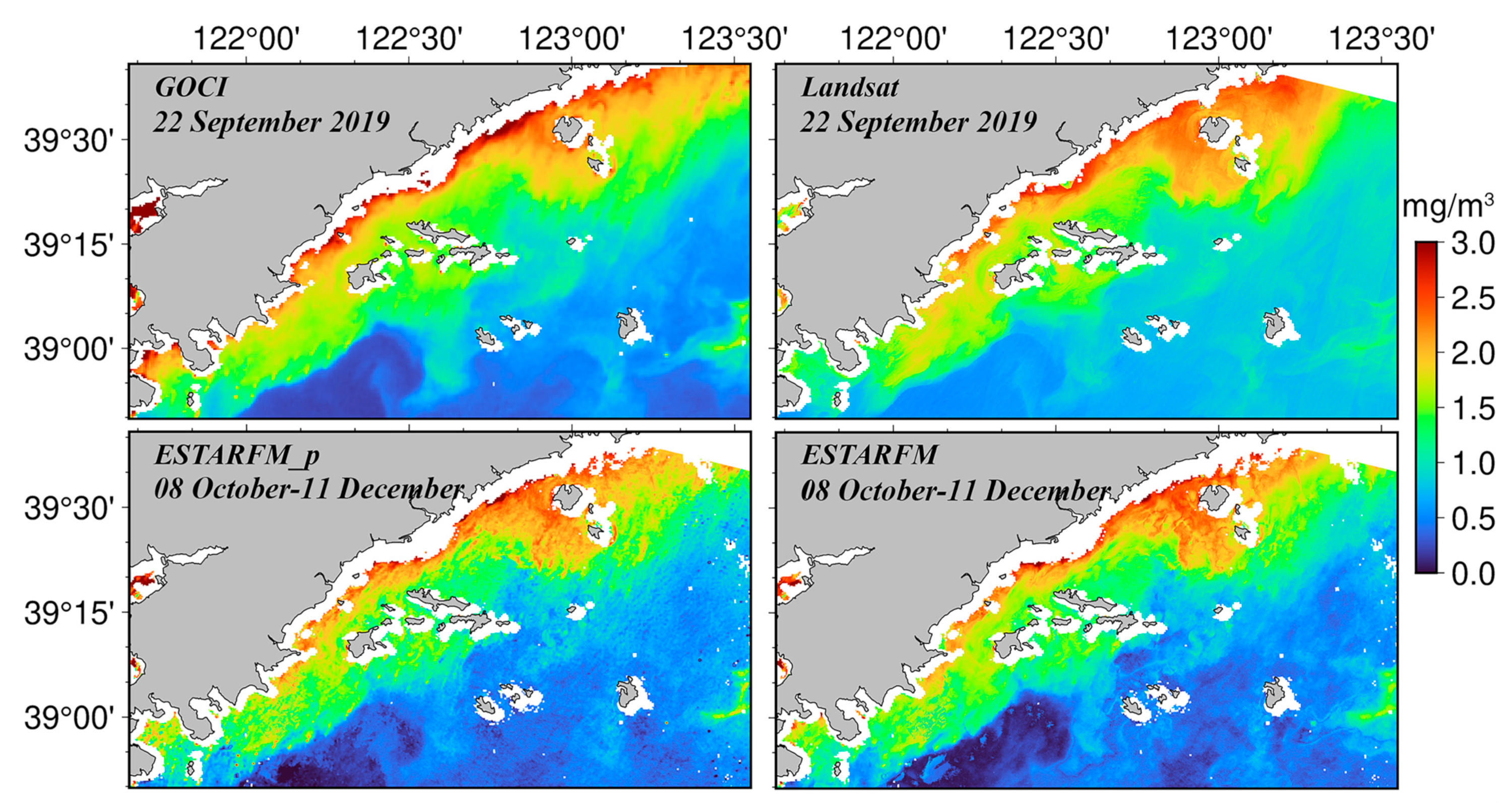
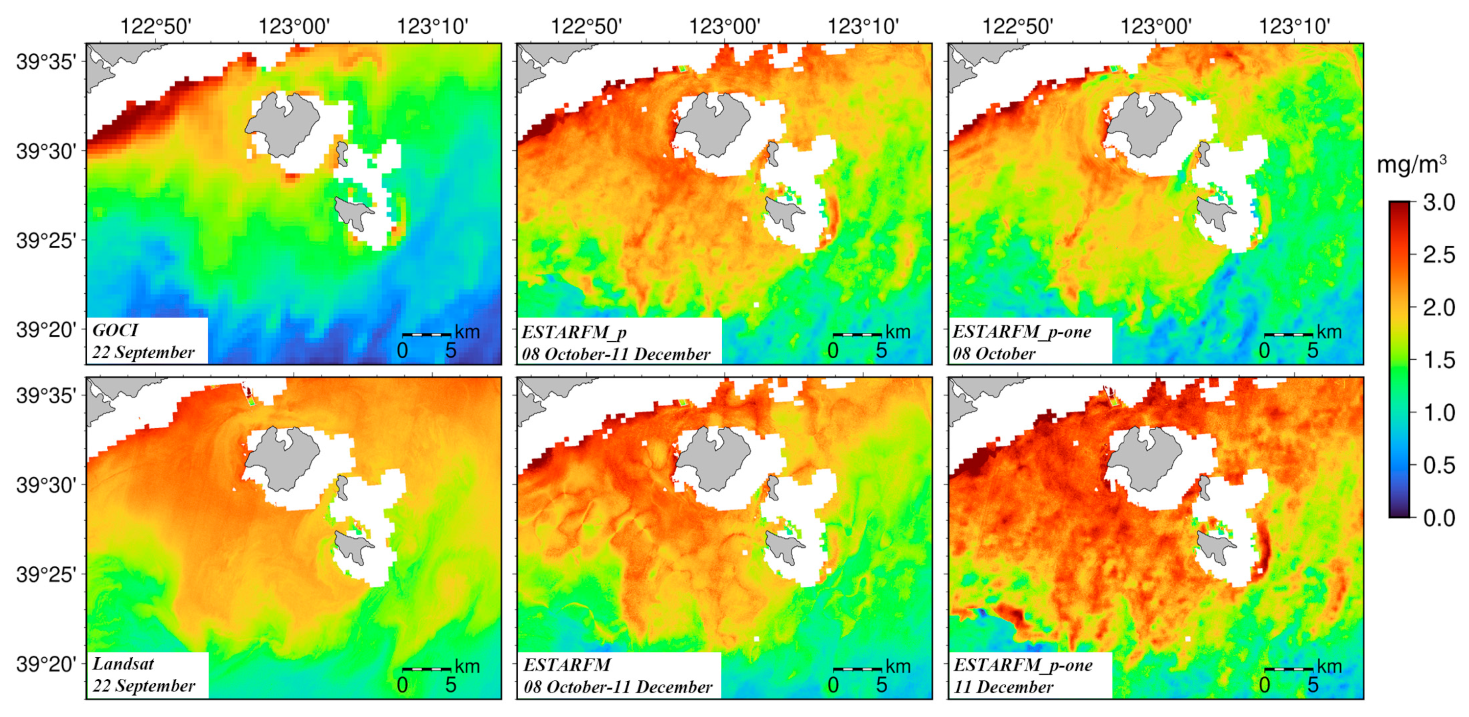
The resulting images are shown in Figure 5. The upper two pictures are the Chl-a data retrieved from GOCI and Landsat images taken on 22 September 2019. The bottom two pictures are the results of the ESTARFM and ESTARFM_p. Compared with the GOCI data, the results of the two fusion models show refined textures, especially in nearshore and areas where the Chl-a concentration changes rapidly. Compared with the Landsat image, the results of the two models show similar spatial distribution, which indicates the information in fine-resolution images is modeled successfully. Both models successfully predicted the Chl-a in the target date. Compared with the results of the new model, the ESTARFM image showed abrupt patterns in some areas, while the new model showed better spatial consistency.
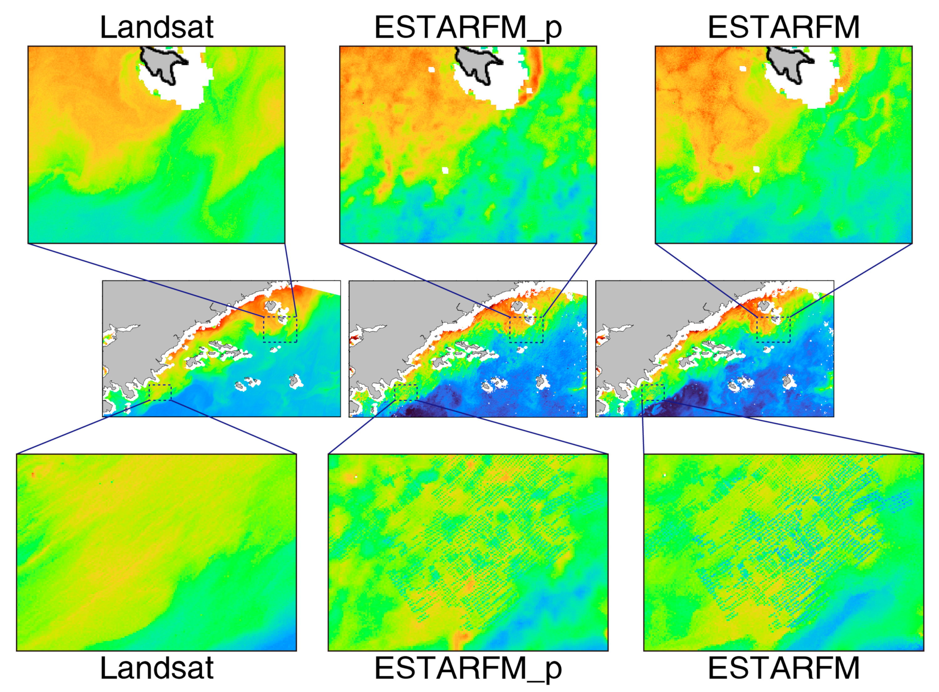
Although the general trends of the results are consistent with the Landsat Chl-a images, the detailed spatial textures are quite different, as shown in Figure 6. The detailed features in Landsat images were caused by the phytoplankton and hydrodynamic conditions on the target date, which are difficult to calculate using the model. The input for the model was only low-resolution data of the target date, and the model cannot directly create details from nothing. The texture characteristics expressed in the results were derived from other high-resolution basic data. For the model, the process can be considered as combining several images to integrate their advantages through a suitable weighting mode. So, it is hard for the models to obtain images as smoothly as the Landsat does. What the model managed to collect was the information of the general trends on spatial and temporal variation. The blue grids on the southwest coast are the aquaculture ponds that were not captured by Landsat on 22 September, while these were captured in the input images. Therefore, obtaining a high-resolution image close to the target date is very important.
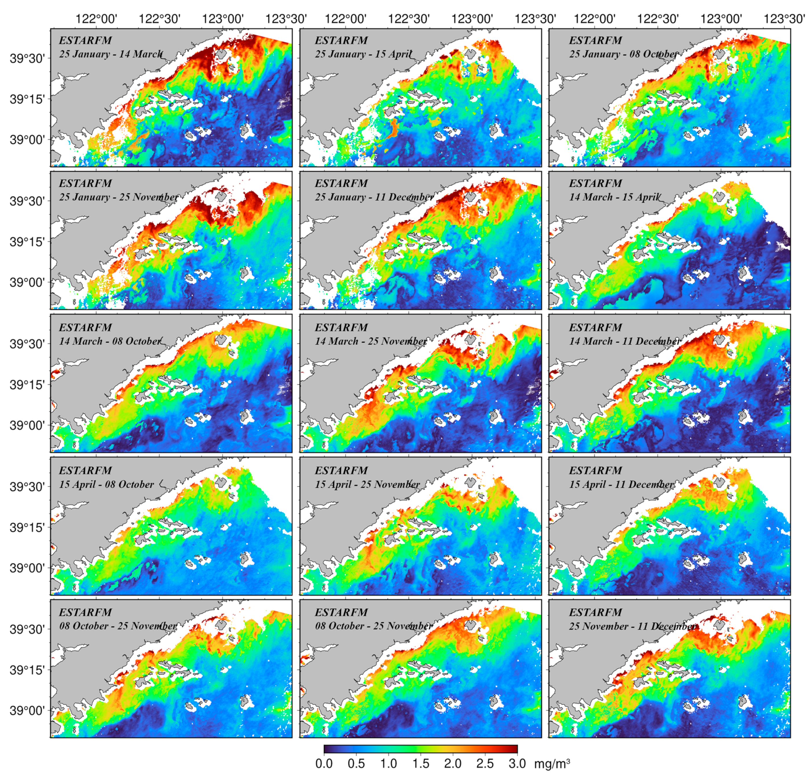
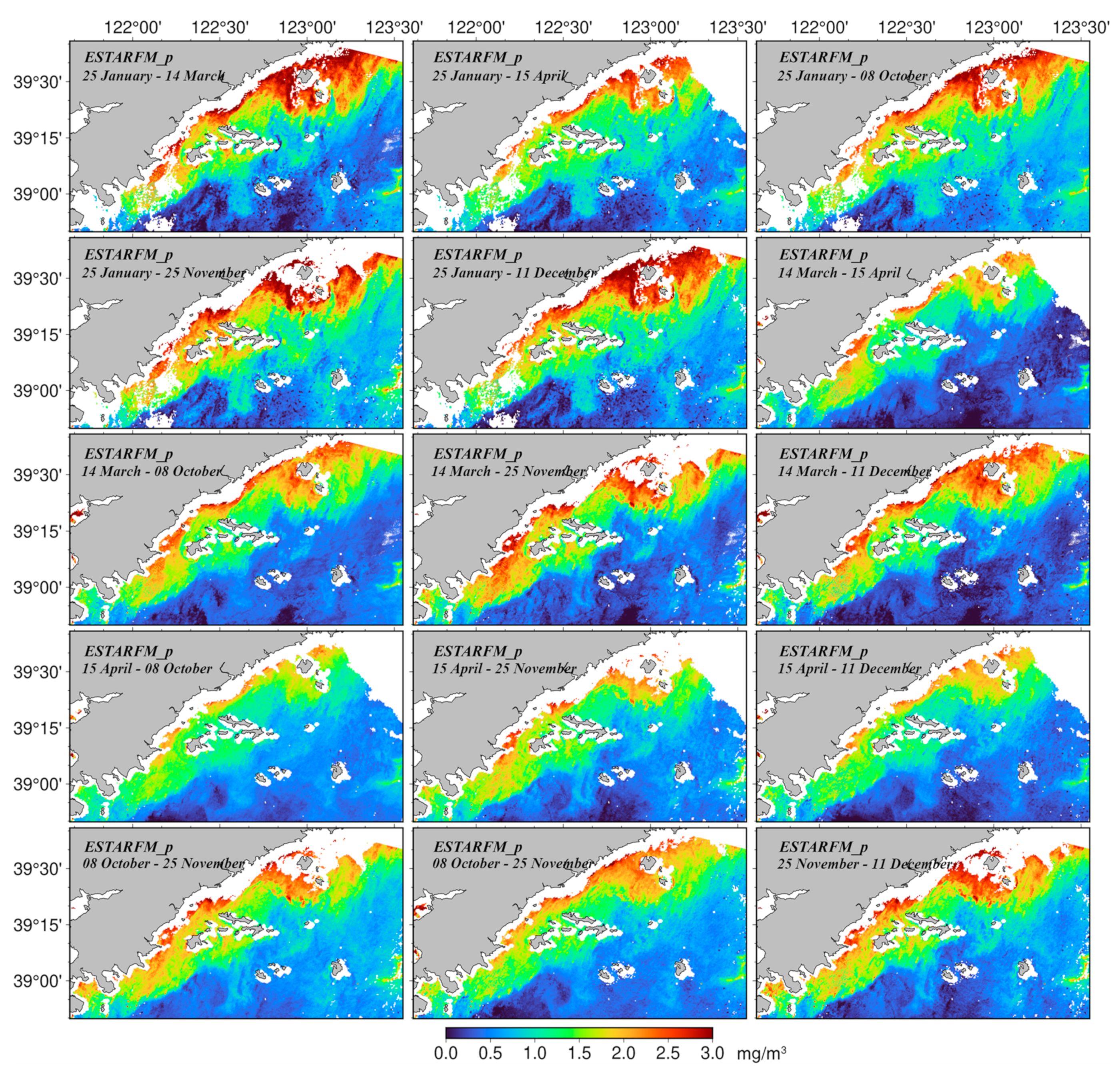
Figure 7 and Figure 8 show the results of the two models for the 15 input groups. The results are identified by the dates of the original images. As can be seen from the images, results for the same target day derived from different original data vary in values and spatial distributions.
The model can only successfully calculate the result when all the basic data are valid values. Therefore, compared with the GOCI data provided, the results of the two models have blank values in some areas, resulting in missing information, which limits the applicability of both models.

4. Discussion

Because of the difference between Chl-a and surface reflection data, as well as the characteristics of rapid changes in Chl-a concentration, this paper used segmented fitting and numerical conversion methods to obtain the target image based on the original assumptions of the ESTARFM.

4.1. The Impact of Limited Input Data on Model Results

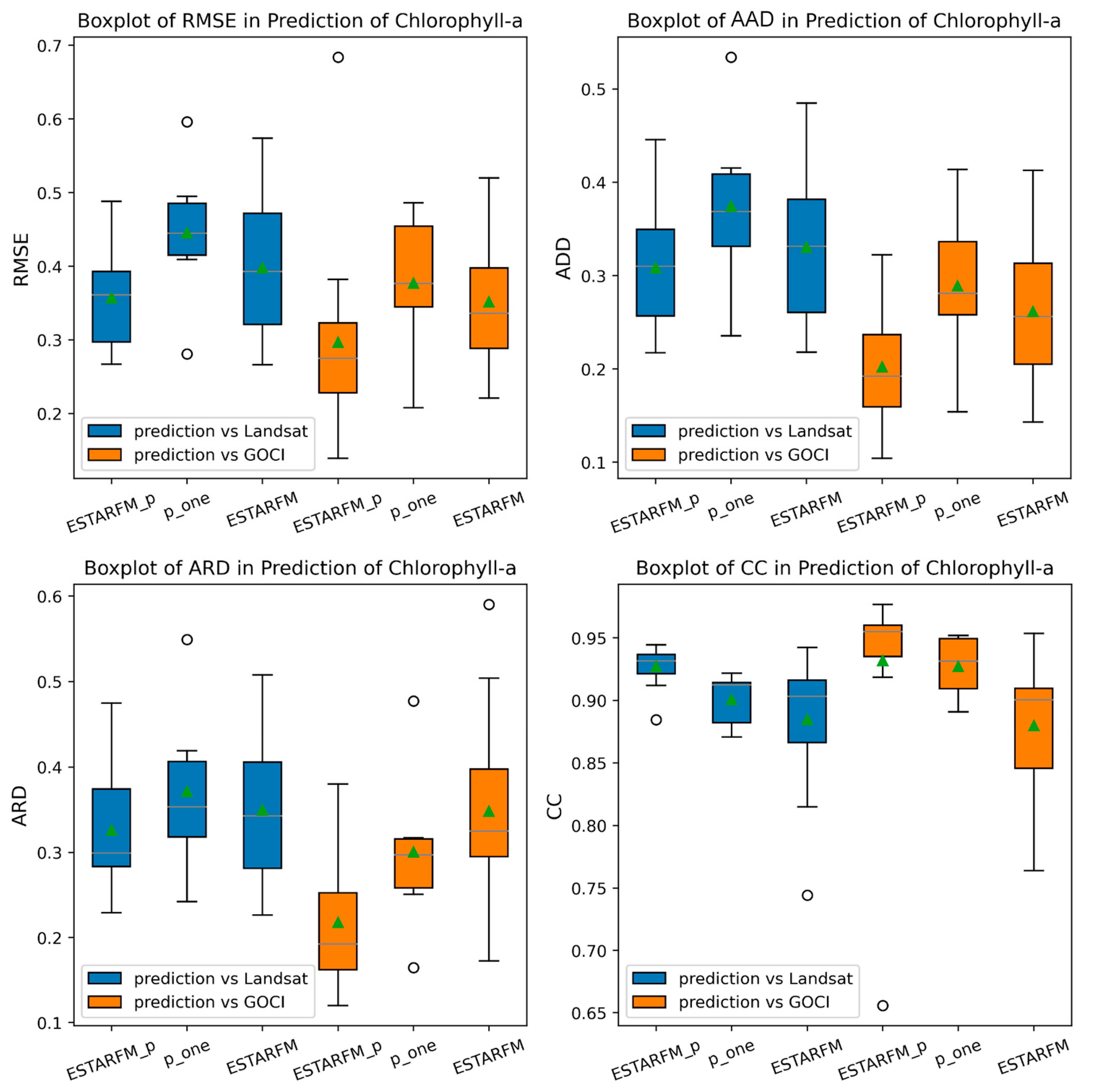
In the ESTARFM, three input images are required. More basic images can provide more information about the changes and make the results more reliable. However, valid data are limited, which severely constrains the application of data fusion. The segmented fitting and numerical conversion process of the ESTARFM_p takes more into account the spatial information of the original images. So, in this section, an attempt was made to test whether the model could handle having a lack of coarse-resolution images on the target date. To quantitatively test the degradation of accuracy when there are fewer inputs, the new model performed predictions with input images on a single date as an extreme case. The input data were the GOCI and Landsat pairs in Table 1, excluding those obtained on 22 September.
The statistical coefficients of the results are shown in Figure 9. Taking the actual observations of Landsat as “true values”, these results were calculated from the 15 different date combinations in Table 3 and single-date images in Table 1. Compared with the ESTARFM, the new model scheme had a better performance in all the indicators. The reason for this may be that the new model scheme adopts the numerical conversion method, which is more suitable for the characteristics of chlorophyll concentration data. The single-date results also show reasonable coefficients but with more fluctuations and outliers. Compared with the ESTARFM, the single-date results show a higher RMSE and lower CC, which indicates that the number of input images has a great impact on the model results.
To better illustrate this, areas near Shicheng Island and Wangjia Island were extracted, as shown in Figure 10. Compared with the Landsat observations, all three models managed to obtain variations in the Chl-a. The ESTARFM_p performed the best as it did not miss any of the peaks. The single-date model results show abrupt predictions and gaps in both numerical and spatial distribution. However, the general trends are still similar to the remote sensing observations. Therefore, although the accuracy of the model degrades when it lacks inputs, the results of the ESTARFM_p could still be taken into account in engineering problems that need less accuracy.

4.2. The Effect of the Temporal Distance between the Input and the Target on the Model Results

The ESTARFM uses three basic images to calculate the target image. The closer the acquisition time is, the higher the accuracy of the result. Figure 11 shows the changes in the statistical indicators with different time intervals. As the interval increases, the RMSE showed obvious upward trends, while the CC showed downward trends. The two models performed similarly before 130 days. Both ESTARFM indicators fluctuated and degraded after 130 days, with the average RMSE increasing by about 47% and CC decreasing by about 14%. The average ESTARFM_p RMSE degraded within a smaller range (18%), and its CC did not show a significant decrease. Single-date results have similar trends. The CC values were also more stable than those of the ESTARFM. Therefore, the new model in this study is more robust when there are limited input data. The reason for this is that the modified similar-pixel-obtaining process increases the weight of the GOCI data on the target date, and it therefore collects more valid information than the original model does.

4.3. Comparison of Model Applicability

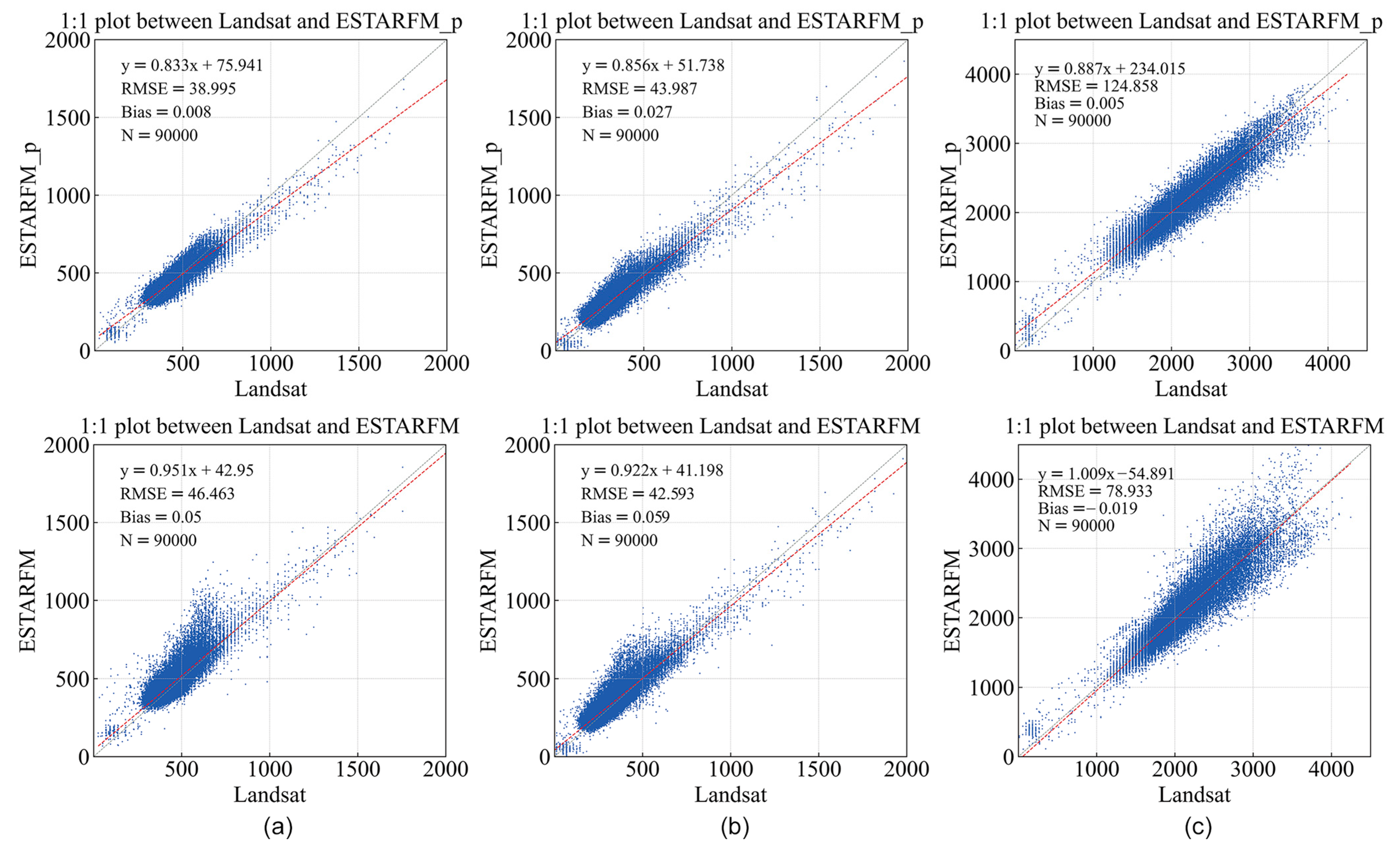
In this section, the new model was applied to the sample data (with changes) shared by the ESTARFM designer to evaluate the performance of the new model on reflectance data [21]. The results are shown in Figure 12.
Upon comparing the results of the two models and the actual observations, the new model was found to obtain values closer to the actual values due to the inclusion of numerical conversion. However, segmented fitting reduces spatial variability. Compared with the ESTARFM, it blurs some spatial details and may cause inconsistency in the image, as seen in the yellow box (a) in Figure 13. The ESTARFM fully expresses the spatial texture through spatial retrieval and conversion.
The results of the reflectance data derived from the two models show that the new model is more suitable for a single type of data with a larger range of variation. For terrestrial areas with sudden changes in land cover types, the ESTARFM scheme is more robust.

4.4. Limitations of the Models

In terms of remote sensing spatiotemporal data fusion, the ESTARFM and the new model still have limitations:
(1) The spatiotemporal data fusion model is data-driven. Therefore, it is difficult for it to accurately generate details and textures that only exist on the target date.
(2) In the process of model calculation, the size of the sliding window and the selection rules of similar pixels are very important. The optimal settings for these parameters still cannot be automatically generated by the program.

5. Conclusions

The monitoring of nearshore Chl-a changes is a critical ecological issue. The purpose of the current study was to design a proper model for remote sensing Chl-a data fusion for coastal environments. Our contributions are as follows:
(1) A modified ESTARFM was proposed to make use of the characteristics of Chl-a data and applied to the northern coast of the Yellow Sea. The spatial resolution of GOCI Chl-a was downscaled to 30 m. The methods were tested with actual satellite data. Both fusion models could obtain reasonable coastal Chl-a.
(2) The predicted results were evaluated visually and statistically. The new model improves the applicability of the spatiotemporal fusion model to the rapidly changing Chl-a data. Compared with the ESTARFM results, the new model results have a more stable indicator performance and better spatial consistency. This shows that the method of segmented fitting and numerical conversion is more suitable for data with rapid changes in spatial distribution.
(3) In the case input data are limited, numerical conversion reduces the impact of time intervals on the model. The results of this study prove that the new model is more stable and robust than the original model. So, the new model has more potential in practical application.

Author Contributions

Conceptualization, Y.F. and J.S.; methodology, Q.M.; software, Q.M.; validation, Y.C.; formal analysis, J.G. and M.L.; writing—original draft preparation, Q.M.; writing—review and editing, Y.F. and X.J. All authors have read and agreed to the published version of the manuscript.

Funding

This work was supported by the Dalian Science and Technology Program for Innovation Talents of Dalian (2022RJ06); the Science and Technology Program of Liaoning Province (2021-BS-239, 2022JH2/101300222, 2022JH2/101300183); the Scientific Research Project of Education Department of Liaoning Province (DL202001, JL202006, QL202006, LJKZ0709); the Open Fund Project of the Key Laboratory of Marine Environmental Information Technology, MNR (Yanzhao Fu); and the Dalian Science and Technology Innovation Fund (2020JJ27SN100).

Data Availability Statement

The data presented in this study are available upon request to the corresponding author.

Acknowledgments

The authors appreciate USGS for providing the Landsat data and KOSC for the GOCI data. We thank the data support from the National Marine Scientific Data Center (Dalian) and the National Science and Technology Infrastructure of China (http://odc.dlou.edu.cn/ (accessed on 2 September 2023)) for providing valuable data and information.

Conflicts of Interest

The authors declare no conflict of interest.

References

  1. Price, J.C. How unique are spectral signature? Remote Sens. Environ. 1994, 49, 181–186. [Google Scholar] [CrossRef]
  2. Masek, J.G.; Huang, C.; Wolfe, R.; Cohen, W.; Hall, F.; Kutler, J.; Nelson, P. North American forest disturbance mapped from a decadal Landsat record. Remote Sens. Environ. 2008, 112, 2914–2926. [Google Scholar] [CrossRef]
  3. Yue, L.; Shen, H.; Li, J.; Yuan, Q.; Zhang, H.; Zhang, L. Image super-resolution: The techniques, applications, and future. Signal Process. 2016, 128, 389–408. [Google Scholar] [CrossRef]
  4. Yang, J.; Wright, J.; Huang, T.S.; Ma, Y. Image super-resolution via sparse representation. IEEE Trans. Image Process. 2010, 19, 2861–2873. [Google Scholar] [CrossRef]
  5. Hui, Z.; Li, J.; Gao, X.; Wang, X. Progressive perception-oriented network for single image super-resolution. Inform. Sci. 2021, 546, 769–786. [Google Scholar] [CrossRef]
  6. Zhang, H.; Yang, Z.; Zhang, L.; Shen, H. Super-Resolution Reconstruction for Multi-Angle Remote Sensing Images Considering Resolution Differences. Remote Sens. 2014, 6, 637–657. [Google Scholar] [CrossRef]
  7. Fisher, J. High spatial resolution sea surface climatology from Landsat thermal infrared data. Remote Sens. Environ. 2004, 90, 293–307. [Google Scholar] [CrossRef]
  8. Miskin, J.; Mackay, D. Ensemble Learning for Blind Image Separation and Deconvolution. In Advances in Independent Component Analysis; Springer: London, UK, 2000. [Google Scholar]
  9. Takeda, H.; Farsiu, S.; Milanfar, P. Kernel Regression for Image Processing and Reconstruction. IEEE T. Image Process. 2007, 16, 349–366. [Google Scholar] [CrossRef]
  10. Dong, C.; Loy, C.C.; He, K.; Tang, X. Image Super-Resolution Using Deep Convolutional Networks. IEEE T. Pattern Anal. 2016, 38, 295–307. [Google Scholar] [CrossRef]
  11. Trinh, D.; Luong, M.; Dibos, F.; Rocchisani, J.; Pham, C.; Nguyen, T.Q. Novel Example-Based Method for Super-Resolution and Denoising of Medical Images. IEEE T. Image Process. 2014, 23, 1882–1895. [Google Scholar] [CrossRef] [PubMed]
  12. Saharia, C.; Ho, J.; Chan, W.; Salimans, T.; Fleet, D.J.; Norouzi, M. Image Super-Resolution via Iterative Refinement. arxiv 2021, arXiv:2104.07636. [Google Scholar] [CrossRef]
  13. Guo, S.; Sun, B.; Zhang, H.K.; Liu, J.; Chen, J.; Wang, J.; Jiang, X.; Yang, Y. MODIS ocean color product downscaling via spatio-temporal fusion and regression: The case of chlorophyll-a in coastal waters. Int. J. Appl. Earth Obs. 2018, 73, 340–361. [Google Scholar] [CrossRef]
  14. Yocky, D.A. Multiresolution wavelet decomposition image merger of Landsat Thematic Mapper and SPOT panchromatic data. Photogramm. Eng. Remote Sens. 1996, 62, 1067–1074. [Google Scholar]
  15. Nunez, J.; Otazu, X.; Fors, O.; Prades, A.; Pala, V.; Arbiol, R. Multiresolution-based image fusion with additive wavelet decomposition. IEEE T. Geosci. Remote 1999, 37, 1204–1211. [Google Scholar] [CrossRef]
  16. Zhang, H.K.; Huang, B.; Zhang, M.; Cao, K.; Yu, L. A generalization of spatial and temporal fusion methods for remotely sensed surface parameters. Int. J. Remote Sens. 2015, 36, 4411–4445. [Google Scholar] [CrossRef]
  17. Gao, F.; Masek, J.; Schwaller, M.; Hall, F. On the blending of the Landsat and MODIS surface reflectance: Predicting daily Landsat surface reflectance. IEEE T. Geosci. Remote 2006, 44, 2207–2218. [Google Scholar]
  18. Hilker, T.; Wulder, M.A.; Coops, N.C.; Linke, J.; McDermid, G.; Masek, J.G.; Gao, F.; White, J.C. A new data fusion model for high spatial- and temporal-resolution mapping of forest disturbance based on Landsat and MODIS. Remote Sens. Environ. 2009, 113, 1613–1627. [Google Scholar] [CrossRef]
  19. Zhang, B.; Zhang, L.; Xie, D.; Yin, X.; Liu, C.; Liu, G. Application of Synthetic NDVI Time Series Blended from Landsat and MODIS Data for Grassland Biomass Estimation. Remote Sens. 2016, 8, 10. [Google Scholar] [CrossRef]
  20. Gao, F.; Anderson, M.C.; Zhang, X.; Yang, Z.; Alfieri, J.G.; Kustas, W.P.; Mueller, R.; Johnson, D.M.; Prueger, J.H. Toward mapping crop progress at field scales through fusion of Landsat and MODIS imagery. Remote Sens. Environ. 2017, 188, 9–25. [Google Scholar] [CrossRef]
  21. Zhu, X.; Chen, J.; Gao, F.; Chen, X.; Masek, J.G. An enhanced spatial and temporal adaptive reflectance fusion model for complex heterogeneous regions. Remote Sens. Environ. 2010, 114, 2610–2623. [Google Scholar] [CrossRef]
  22. Huang, B.; Zhang, H. Spatio-temporal reflectance fusion via unmixing: Accounting for both phenological and land-cover changes. Int. J. Remote Sens. 2014, 35, 6213–6233. [Google Scholar] [CrossRef]
  23. Bai, L.; Cai, J.; Liu, Y.; Chen, H.; Zhang, B.; Huang, L. Responses of field evapotranspiration to the changes of cropping pattern and groundwater depth in large irrigation district of Yellow River basin. Agr. Water Manag. 2017, 188, 1–11. [Google Scholar] [CrossRef]
  24. Pan, Y.; Shen, F.; Wei, X. Fusion of Landsat-8/OLI and GOCI Data for Hourly Mapping of Suspended Particulate Matter at High Spatial Resolution: A Case Study in the Yangtze (Changjiang) Estuary. Remote Sens. 2018, 10, 158. [Google Scholar] [CrossRef]
  25. Honeywill, C.; Paterson, D.M.; Hagerthey, S.E. Determination of microphytobenthic biomass using pulse-amplitude modulated minimum fluorescence. Eur. J. Phycol. 2002, 37, 485–492. [Google Scholar] [CrossRef]
  26. Gao, J.; Shi, H.; Zang, J.; Liu, Y. Mechanism analysis on the mitigation of harbor resonance by periodic undulating topography. Ocean Eng. 2023, 281, 114923. [Google Scholar] [CrossRef]
  27. Gao, J.; Ma, X.; Dong, G.; Chen, H.; Liu, Q.; Zang, J. Investigation on the effects of Bragg reflection on harbor oscillations. Coastal Eng. 2021, 170, 103977. [Google Scholar] [CrossRef]
  28. Gernez, P.; Doxaran, D.; Barillé, L. Shellfish Aquaculture from Space: Potential of Sentinel2 to Monitor Tide-Driven Changes in Turbidity, Chlorophyll Concentration and Oyster Physiological Response at the Scale of an Oyster Farm. Front. Mar. Sci. 2017, 4, 137. [Google Scholar] [CrossRef]
  29. Harvey, E.T.; Kratzer, S.; Philipson, P. Satellite-based water quality monitoring for improved spatial and temporal retrieval of chlorophyll-a in coastal waters. Remote Sens. Environ. 2015, 158, 417–430. [Google Scholar] [CrossRef]
  30. Kahru, M.; Kudela, R.M.; Lorenzo, E.D.; Manzano-Saraba, M.; Mitchell, B.G. Trends in the surface chlorophyll of the California Current: Merging data from multiple ocean color satellites. Deep Sea Res. Part II Top. Stud. Oceanogr. 2012, 77–80, 89–98. [Google Scholar] [CrossRef]
  31. Gregg, W.W.; Conkright, M.E. Global seasonal climatologies of ocean chlorophyll; blending in situ and satellite data for the Coastal Zone Color Scanner era. J. Geophys. Res. Ocean. 2001, 106, 2499–2515. [Google Scholar] [CrossRef]
  32. Wang, B.; Wang, X.; Zhan, R. Nutrient conditions in the Yellow Sea and the East China Sea. Estuar. Coast. Shelf Sci. 2003, 58, 127–136. [Google Scholar] [CrossRef]
  33. Zhang, H.; Shi, X.; Zhang, C.; Wang, L.I.S. Distribution Features of Nutrients Structure and Nutrient Limitation in the North of Yellow Sea. Period. Ocean. Univ. China 2009, 39, 8. [Google Scholar]
  34. Li, Y.W.; Hu, Y.Y.; Chen, S. Distribution and influence factors of nutrients in the North Yellow Sea in Summer and Autumn. China Environ. Sci. 2013, 33, 1060–1067. [Google Scholar]
  35. Wu, Y.; Zhang, J.; Zhao, L.; Chen, C. Spatiotemporal Characteristics of Nitrogen and Phosphorus and Its Influencing Processes in the Yellow Sea. J. Tianjin Univ. Sci. Technol. 2021, 36, 30–40. [Google Scholar]
  36. Ahn, J.; Park, Y.; Ryu, J.; Lee, B.; Oh, I.S. Development of atmospheric correction algorithm for Geostationary Ocean Color Imager (GOCI). Ocean. Sci. J. 2012, 47, 247–259. [Google Scholar] [CrossRef]
  37. Gordon, H.R.; Wang, M. Retrieval of water-leaving radiance and aerosol optical thickness over the oceans with SeaWiFS: A preliminary algorithm. Appl. Opt. 1994, 33, 443–452. [Google Scholar] [CrossRef]
  38. Gordon, H.R.; Wang, M. Influence of oceanic whitecaps on atmospheric correction of ocean-color sensors. Appl. Opt. 1994, 33, 7754–7763. [Google Scholar] [CrossRef]
  39. Kotchenova, S.Y.; Vermote, E.F.; Matarrese, R.; Klemm, J.F.J. Validation of a vector version of the 6S radiative transfer code for atmospheric correction of satellite data. Part I: Path radiance. Appl. Opt. 2006, 45, 6762–6774. [Google Scholar] [CrossRef]
  40. Kotchenova, S.Y.; Vermote, E.F. Validation of a vector version of the 6S radiative transfer code for atmospheric correction of satellite data. Part II. Homogeneous Lambertian and anisotropic surfaces. Appl. Opt. 2007, 46, 4455–4464. [Google Scholar] [CrossRef] [PubMed]
Figure 1. Study area: Changhai County and Shicheng Island in the northern part of the North Yellow Sea.
Water 15 03566 g001
Figure 2. Overall workflow in this study.
Water 15 03566 g002
Figure 3. The same spatial index is used to process GOCI and Landsat data.
Water 15 03566 g003
Figure 4. Scatter plot comparing the Landsat data with the GOCI and results of the two models.
Water 15 03566 g004
Figure 5. Comparison of the results derived from the images of 8 October and 11 December.
Water 15 03566 g005
Figure 6. Details of the results of ESTARFM and ESTARFM_p.
Water 15 03566 g006
Figure 7. Fifteen sets of Chl-a results for 22 September derived using the ESTARFM.
Water 15 03566 g007
Figure 8. Fifteen sets of Chl-a results for 22 September derived using the ESTARFM-p model.
Water 15 03566 g008
Figure 9. The statistical coefficients of the results of ESTARFM, ESTARFM_p, and ESTARFM_p with single-date inputs (p_one).
Water 15 03566 g009
Figure 10. Detailed comparison of the areas near Shicheng Island and Wangjia Island.
Water 15 03566 g010
Figure 11. The variation in RMSE and CC of ESTARFM, ESTARFM_p, and ESTARFM_p-one results with time intervals.
Water 15 03566 g011
Figure 12. Scatter plots of the Landsat and results of ESTARFM and ESTARFM_p for green (a), red (b), and NIR-infrared bands (c).
Water 15 03566 g012
Figure 13. Comparison of Landsat actual reflectance image, ESTARFM_p, and ESTARFM results.
Water 15 03566 g013
Table 1. Data list of Landsat 8 OLI and GOCI used in this study.
DatePlatform/SensorTime
25 January 2019Landsat/GOCI10:30
14 March 2019Landsat/GOCI10:30
15 April 2019Landsat/GOCI10:30
22 September 2019Landsat/GOCI10:30
8 October 2019Landsat/GOCI10:30
25 November 2019Landsat/GOCI10:30
11 December 2019Landsat/GOCI10:30
Table 2. The coefficients of OC3 and OC3g.
a0a1a2a3a4
OC30.2412−2.05461.1776−0.5538−0.4570
OC3g0.0831−1.99410.56290.2944−0.5458
Table 3. The combination of input data.
Date25 Jan14 Mar15 Apr8 Oct25 Nov
14 March14 March–25 January
15 April15 April–25 January15 April–14 March
8 October8 October–25 January8 October–14 March8 October–15 April
25 November25 November–25 January25 November–14 March25 November–15 April25 November–8 October
11 December11 December–25 January11 December–14 March11 December–15 April11 December–8 October11 December–25 November
Disclaimer/Publisher’s Note: The statements, opinions and data contained in all publications are solely those of the individual author(s) and contributor(s) and not of MDPI and/or the editor(s). MDPI and/or the editor(s) disclaim responsibility for any injury to people or property resulting from any ideas, methods, instructions or products referred to in the content.