RLNformer: A Rainfall Levels Nowcasting Model Based on Conv1D_Transformer for the Northern Xinjiang Area of China

Abstract

Accurate precipitation forecasting is of great significance to social life and economic activities. Due to the influence of various factors such as topography, climate, and altitude, the precipitation in semi-arid and arid areas shows the characteristics of large fluctuation, short duration, and low probability of occurrence. Therefore, it is highly challenging to accurately predict precipitation in the northern Xinjiang area of China, which is located in the semi-arid and arid climate region. In this study, six meteorological stations in the northern Xinjiang area were selected as the research area. Due to the high volatility of rainfall in this area, the rainfall was divided into four levels, namely, “no rain”, “light rain”, “moderate rain”, and “heavy rain and above”, for rainfall level prediction. In order to improve the prediction performance, this study proposed a rainfall levels nowcasting model based on Conv1D_Transformer (RLNformer). Firstly, the maximum information coefficient (MIC) method was used for feature selection and sliding the data, that is, the data of the first 24 h were used to predict the rainfall levels in the next 3 h. Then, the Conv1D layer was used to replace the word-embedding layer of the transformer, enabling it to extract the relationships between features of time series data and allowing multi-head attention to better capture contextual information in the input sequence. Additionally, a normalization layer was placed before the multi-head attention layer to ensure that the input data had an appropriate scale and normalization, thereby reducing the sensitivity of the model to the distribution of input data and helping to improve model performance. To verify the effectiveness and generalization of the proposed model, the same experiments were conducted on the Indian public dataset, and seven models were selected as benchmark models. Compared with the benchmark models, RLNformer achieved the highest accuracy on both datasets, which were 96.41% and 88.95%, respectively. It also had higher accuracy in the prediction of each category, especially the minority category, which has certain reference significance and practical value.

1. Introduction

Accurate and timely precipitation forecasting is of great significance for daily life and production planning, providing early warnings for flood and drought disasters, fllod and drought prevention and control management, etc. However, rainfall is the result of the interaction of multi-scale atmospheric systems and is affected by various environmental factors such as heat, flow fields, and topography [1]. Therefore, precipitation nowcasting is extremely challenging. Although the northern Xinjiang area of China, located in arid and semi-arid areas, experiences scarce rainfall, it has been subject to frequent extreme rainfall events due to factors such as global warming. As a result, people’s lives and property are under certain threats. Therefore, accurate and timely rainfall prediction in this region is crucial for human life and production activities.

Rainfall forecasting can be divided into nowcasting, short-term forecasting, and medium and long-term forecasting, according to the length of the forecast time. Due to long-term development, the forecasting capabilities of medium and long-term forecasting have been significantly improved, but the development of nowcasting and short-term forecasting is obviously insufficient and has major shortcomings. In addition, with the development of the economy, precipitation nowcasting has fallen into line more with people’s needs. In order to further improve the accuracy and stability of precipitation prediction, various methods have been proposed. At present, precipitation prediction methods are mainly divided into data extrapolation methods, traditional statistical methods, machine learning methods, and deep learning methods. Data extrapolation techniques primarily utilize satellite cloud images and meteorological radar detection data to conduct rainfall forecasting. Ryu et al. [2] obtained an initial vector field through a variational echo tracking algorithm and then updated the vector field by solving the Burgers equation. Nizar et al. [3] extracted feature values from the relationship graphs generated from the cloud top temperatures and effective radii of cloud particles obtained from satellite images at different times and used logistic regression to find the probability relationship between these feature values and extreme rainfall events in measured rainfall, enabling the prediction of extreme rainfall events more than 6 hours in advance. Zhu et al. [4] proposed a rain-type adaptive pyramid Kanade–Lucas-Tomasi (A-PKLT) optical flow method for radar echo extrapolation, which divides the rainfall into six types, addressing the difficulty of the PKLT optical flow algorithm in calculating motion vectors in mixed-type rainfall. Methods based on data extrapolation have advantages such as low computational load, fast calculation speed, and the ability to meet real-time forecasting needs, but they do not consider the nonlinear processes of large-scale aerodynamics and thermodynamics, making it difficult to describe complex rainfall processes. For statistical models, traditional time series methods have been widely used and studied, including autoregressive (AR), moving average (MA), and autoregressive integrated moving average (ARIMA). De Luca et al. [5] proposed a hybrid model PRAISE-MET based on stochastic models and numerical weather prediction models, characterized by its advantage in improving rainfall forecasting at the basin scale. D.K. Dwivedi et al. [6] used the method of moments to obtain the probability distribution of monthly rainfall and used the ARIMA model to predict rainfall, which had a minimum root mean square value, and found that the residuals were not relevant. Ray et al. [7] proposed a surface temperature prediction framework using the two-state Markov chain method and the autoregressive method and found that there is a strong correlation between surface temperature and rainfall. Islam et al. [8] used a new hybrid GEP-ARIMAX model to predict rainfall at 12 rainfall stations in Western Australia. Compared with traditional linear and nonlinear models, this model has good rainfall forecasting capabilities. The above studies are based on historical rainfall series prediction, which has the advantages of small calculation amount, simple linear prediction, and high accuracy. However, under strong convective weather conditions, short-term rainfall changes rapidly, and traditional statistical methods have limited accuracy in precipitation nowcasting.

With the development of computer technology, machine learning methods have become an excellent prediction tool, bringing unprecedented opportunities to advance predictions, and can be used for precipitation forecasting. Zhao et al. [9] proposed an hourly rainfall forecasting model (HRF) based on a supervised learning algorithm, compared it with similar work in previous studies, and found that the proposed HRF model has impressive performance in terms of temporal resolution and prediction accuracy. Song et al. [10] proposed a new machine-learning-based model for summer hourly precipitation forecasting in the Eastern Alps, demonstrating that machine learning methods are a promising approach for precipitation forecasting. Maliyeckel et al. [11] used the LightGBM and SVM integrated model to make predictions using the preprocessed dataset. Compared with a single model, the root mean square error of the hybrid model was the smallest and the rainfall prediction results were more accurate. Diez-Sierra et al. [12] evaluated the performance of eight statistical and machine learning methods for long-term daily rainfall prediction in a semi-arid climate region and found that the performance of most machine learning models is very sensitive to hyperparameters and the performance of neural networks is optimal. Appiah-Badu et al. [13] used multiple machine learning methods to predict rainfall in different ecological zones in Ghana and found that random forest, extreme gradient boosting, and multi-layer perceptron performed well, while K-NN performed the worst. Pirone et al. [14] conducted probabilistic rainfall nowcasting for 19 meteorological stations in southern Italy, ranging from 30 min to 6 h in 10-min intervals. They found that the use of temporal and spatial information allowed the model to predict short-term rainfall amounts using only current measurements as input. Raval et al. [15] developed an optimized neural network for comparison with machine learning methods and found that both traditional machine learning models and neural network-based machine learning models can accurately predict rainfall. Adaryani et al. [16] improved the performance of rainfall prediction methods based on PSO-SVR and LSTM by 3–15% and 2–10%, respectively. Rahman et al. [17] proposed a new smart city real-time rainfall prediction system using machine learning fusion technology, making the prediction results better than other models. Although the machine learning model can effectively fit the implicit nonlinear relationship between historical data and external factors, there are still some shortcomings, such as local optimum, dependence on manual parameter adjustment, and being prone to over-fitting.

In recent years, deep learning has demonstrated extraordinary capabilities and huge potential in many different fields, making breakthroughs in the fields of computer vision, speech recognition, and natural language processing. New technological innovation brings both challenges and opportunities to the development of weather forecasting technology. Deep learning provides new methods for meteorological problems that are difficult to solve based on shallow neural networks. Amini et al. [18] developed several deep neural networks (DNNs) for rainfall nowcasting with a lead time of 5 min. They integrated the predictions from these DNNs with the forecasts from some numerical weather prediction models using three ensemble methods, thereby enhancing the prediction accuracy. Khaniani et al. [19] used MLP and nonlinear autoregressive (NARX) with exogenous inputs to predict precipitation in Tehran, respectively, and the NARX model showed better performance than MLP in both non-rainfall and rainfall event prediction. Li et al. [20] developed a neural network method with seven meteorological variables as input data based on the backpropagation (BP) algorithm to detect heavy precipitation, which was superior to existing models. Bhimavarapu et al. [21] proposed an enhanced regularization function to predict rainfall to reduce bias, and the performance of the proposed IRF-LSTM surpassed the state-of-the-art methods. Fernández et al. [22] proposed a novel architecture, Broad-Unet, based on the core UNet model. This model learns more complex patterns by combining multi-scale features. Compared to the core UNet model, it not only has fewer parameters but also boasts higher prediction accuracy. Zhang et al. [23] proposed a combined surface and upper-altitude rainfall forecasting model (ACRF) and tested it on 92 weather stations in China and found that ACRF outperformed existing methods in terms of threat score and MSE. Khan et al. [24] confirmed that the Conv1D-MLP hybrid model is more effective at capturing the complex relationship between causal variables and daily variation in rainfall. Zhang et al. [25] used the K-means clustering method to divide the samples into four types, and each type was modeled by LSTM separately, which reduced the root mean square error by 0.65 and improved the threat scores of light rain and heavy rain. Yan et al. [26] proposed a rainfall forecasting model based on TabNet, using 5-year meteorological data from 26 stations in the Beijing–Tianjin–Hebei region to verify that the proposed rainfall forecasting model has good forecasting performance. Due to differences in region and climate, although the above research has achieved relatively ideal results, it is not necessarily applicable to the research tasks of this paper. Since meteorological data comprise a collection of data arranged in chronological order, they can be regarded as time series data. Time series data are characterized by time dependence. Numerous time series models [27,28,29,30] based on deep learning have been developed for time series prediction. The characteristic of these time series models is that they can capture the long-term dependence of the sequence and improve prediction performance. Time series models have been widely used in fields such as short-term load forecasting [31,32,33], but their applications in the meteorological field are relatively rare.

Currently, data used for rainfall nowcasting primarily consist of satellite cloud images and radar images due to their advantages of wide coverage, real-time updates, and high spatio-temporal resolution. However, when compared to data from ground meteorological stations, they have limitations such as accuracy being affected by terrain, significant estimation errors, and inability to capture small-scale precipitation variations. Moreover, deep learning models currently used for rainfall nowcasting predominantly involve recurrent neural networks (RNN) and their variants, as well as hybrid models combining convolutional neural networks (CNN) and RNN. Nevertheless, RNNs have drawbacks like susceptibility to gradient vanishing or exploding; inability to parallelize computations, leading to lower operational efficiency; and challenges at capturing long-term contextual relationships. While the transformer and its variants have effectively addressed the limitations of RNNs, they have mainly been used to solve long-term dependency issues and have not been widely adopted in the domain of rainfall nowcasting. Therefore, inspired by the limitations of satellite cloud images and radar images, as well as the extensive application of the transformer in various domains, this paper selects six meteorological stations in the northern Xinjiang area as the study area. We integrate CNN and the transformer to construct a rainfall nowcasting model based on Conv1D_Transformer, named RLNformer.

The contributions of this study are as follows:

(1)

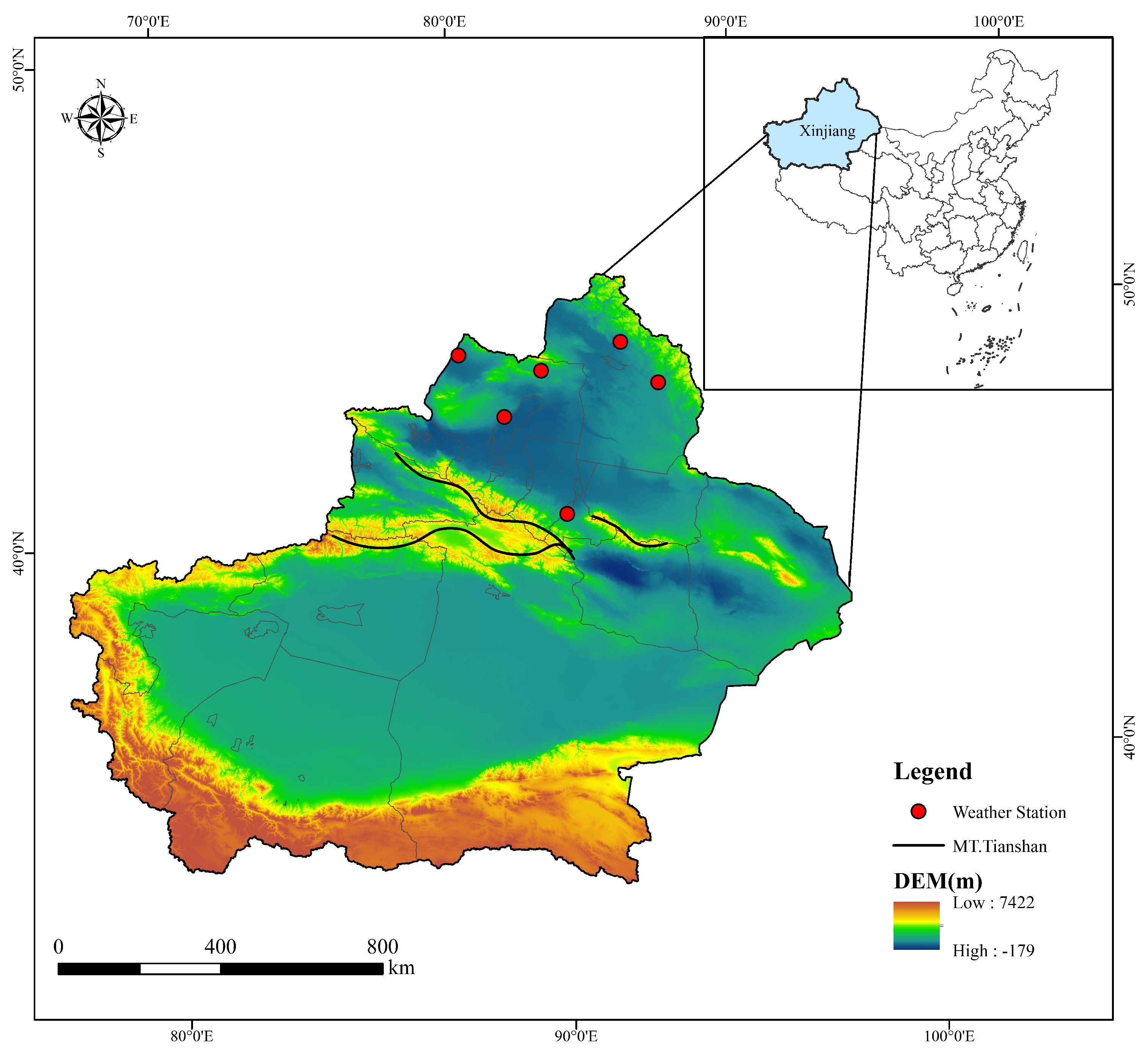
Innovatively, we chose data from six ground meteorological stations in the northern Xinjiang area instead of radar images as the dataset for rainfall nowcasting. The accuracy of ground meteorological station data is higher on a smaller scale, ensuring the precision of the training data.

(2)

The preprocessed dataset can provide a reference for future research. In this paper, comprehensive preprocessing was conducted on the raw data, with a particular focus on complex feature construction. This increased the diversity of the data, improved its quality, and ensured data consistency. The dataset can serve as a foundation for future studies on rainfall nowcasting in the same area, allowing for further analysis and research based on this groundwork.

(2)

The RLNformer model suitable for rainfall nowcasting was constructed. The RLNformer model overcomes the drawbacks of using RNN models for rainfall nowcasting, and its included residual structure mitigates the gradient vanishing or exploding issues present in RNN models to a certain extent. Furthermore, the RLNformer model employs Conv1D to replace the word-embedding layer of the transformer, enabling it to fully capture the complex relationships between temporal features. This allows the attention mechanism to extract the context information of the input data more effectively, enhancing predictive performance. This structure resolves the issues of the inability to process inputs in parallel and difficulties at capturing long-term contextual dependencies, which are present in RNN-based rainfall nowcasting models. Lastly, the original transformer’s normalization layer is placed before the multi-head attention, ensuring that the extracted features have an appropriate scale, which enhances the model’s stability. The prediction results of the model on two datasets indicate that transformer-based models are equally suitable for rainfall nowcasting tasks.

2. Study Area and Data Preprocessing

2.1. Study Area

Semi-arid and arid areas [34] refer to regions where the ratio of average annual precipitation to annual potential evaporation is between 0.2 and 0.5. The characteristics of semi-arid and arid areas are low rainfall, scarce water resources, and grassland vegetation as the main natural vegetation. China’s northwest region is mostly located in semi-arid and arid areas, and the northern Xinjiang area is a typical semi-arid and arid area with an average annual precipitation of about 200 mm. This paper selects 6 meteorological stations in the northern Xinjiang area as the target study area. The distribution of the study area’s stations is shown in Figure 1, and the information of each meteorological station is shown in

Table 1. Weather stations information.

Station No.	Latitude (°)	Longitude (°)	Altitude (m)
51076	47.73	88.08	735.3
51087	46.98	89.52	807.5
51133	46.73	83.00	534.9
51156	46.78	85.72	1322.1
51243	45.62	84.85	450.3
51463	43.78	87.37	935.0

.

It can be seen from the stations distribution and station information that the longitude, latitude, and altitude of each station in the study area are quite different, which makes the rainfall patterns of each site diversified. Therefore, it is extremely challenging to conduct accurate and timely rainfall prediction research on meteorological stations in northern Xinjiang.

2.2. Original Data

The data used in this study were downloaded from the meteorological website (https://rp5.ru/, accessed on 20 May 2023). This dataset covers the historical meteorological data of 6 meteorological stations in northern Xinjiang from 1 February 2005 to 31 July 2023. Each meteorological station data has 18 features, of which one feature is the date feature and the rest are meteorological features. All of the features are recorded every 3 h. The specific information of the date characteristics and meteorological characteristics of the original data set is shown in

Table 2. Original feature information.

Number	Feature	Description	Unit
1	Date	Date of record	/
2	T	Temperature 2 m above ground	℃
3	Po	Horizontal atmospheric pressure	mmHg
4	P	Mean sea level pressure	mmHg
5	Pa	The change of atmospheric pressure within 3 h before observation	mmHg
6	U	Relative humidity at 2 m above the ground	%
7	DD	The wind direction 10–12 m above the ground within 10 min before observation	/
8	Ff	The wind speed 10–12 m above the ground within 10 min before observation	m/s
9	ff10	The maximum gust 10–12 m above the ground within 10 min before observation	m/s
10	N	The maximum gust 10–12 m above the ground between the two observations	m/s
11	N	Total cloud cover	/
12	Tn	Minimum air temperature	℃
13	Tx	Maximum air temperature	℃
14	H	The height of the lowest cloud	m
15	VV	Horizontal visibility	km
16	Td	Dew point temperature at 2 m above ground	℃
17	RRR	Precipitation within 3 h	mm
18	Tg	The lowest temperature of soil surface at night	℃

.

2.3. Data Preprocessing

2.3.1. Data Cleaning

Due to meteorological equipment failures, data storage, and other reasons, the original data are missing, and some features have a large number of continuous missing values. If these missing values are filled in, a lot of noise will be introduced, affecting model predictions. First of all, after statistics on rainfall characteristic values, it was found that nearly 80% of the data were missing. Therefore, the data from 1 January 2020 to 31 July 2023 were screened out as research data. Next, a statistical analysis was performed on the proportion of missing values for other meteorological feature values at each meteorological station. It was found that the proportion of missing values for the characteristics ff10, N, H, and Tg of each meteorological station ranged from 25% to 100%, and the missing values were all distributed within a continuous period of time. Therefore, the above four features are deleted, and 14 features are finally retained as original features.

2.3.2. Outliers and Missing Values Handling

Abnormal values are mainly caused by actual values exceeding the maximum value of the measuring instrument. Outliers in meteorological data are usually represented by relatively large integers. Through exploratory data analysis (EDA), it was found that there are no outliers in any of the features of each meteorological station; through statistical analysis, it was found that some features in the original dataset had a small number of missing values. If they were deleted directly, other valuable data would be lost. In order to reduce information loss and ensure data integrity as much as possible, missing values are filled. Since different features have different proportions of missing feature values, a single filling method cannot be used. For features with a relatively small proportion of missing values, use the mean of the two data before and after as the filling value; for features with a relatively large proportion of missing values and missing data at consecutive time steps, use the multiple imputation method to fill them. The reason for choosing this method is that multiple imputations can improve data utilization and retain the characteristics of the original data, thereby better reflecting the real situation of the data.

The meteorological department defines rainfall less than 0.1 mm within 3 h as micro-rainfall. The impact of micro-rainfall on the northern Xinjiang area, which is located in a semi-arid and arid climate zone, is almost zero, but it will make it difficult for the model to distinguish between no-rainfall and micro-rainfall, which brings great challenges to the rainfall prediction task. Therefore, considering the research area and rainfall prediction task, the value of trace rainfall is set to 0.

2.3.3. Feature Construction

Precipitation is the result of the combined effects of air pressure, temperature, wind direction, and other features. If the number of original features is too small, the model will extract less relevant information from them, resulting in poor prediction results. In order to better extract useful information from the data and enhance the predictive power of the model, the following features are constructed:

• Time features. Precipitation shows different trends in different time periods of the year. Time features can help researchers understand the rainfall pattern in the target area, and the model can also capture changes in precipitation over time, thereby improving prediction performance. This paper uses the date feature Date as an index and splits it into four features, namely, Year, Month, Day, and Time, which, respectively, represent the year, month, day, and hour of the record.
• STL decomposition features. Meteorological data are essentially time series data and have a certain periodicity. STL decomposition [35] can decompose time series data more precisely, that is, decompose time series data into three parts: trend, season, and residual. This can hep one to better understand and analyze the trend, periodicity, and randomness of time series data and enable better prediction and modeling. Therefore, STL decomposition is performed on features related to air temperature, air pressure, relative humidity, wind speed, and precipitation.
• Variation features. Variables such as air pressure, temperature, and humidity generally change during a period of time before rainfall occurs. Therefore, first-order variation features and second-order variation features are introduced for each meteorological feature.
• Interaction features. Precipitation is the result of the interaction of meteorological features, and the interaction between features should be taken into account, for example, the values of temperature and relative humidity are multiplied to obtain another feature.
• Difference features. Using the difference between two features as a new feature can reflect the changes between feature values, allowing the model to better capture the fluctuations in the data.

After feature construction, the number of features increased from 14 to 90.

2.3.4. Data Normalization

In the precipitation dataset used in this paper, the value range of the original data changes greatly, which leads to the dominance of high eigenvalues and the weakening of the influence of low eigenvalues on the model. Therefore, the original data are scaled using the minimum–maximum normalization method to retain its distribution shape and map the data to a fixed range. The calculation formula is as follows.

$$x^{*}=\frac{x-x_{\min }}{x_{\max }-x_{\min }}$$

(1)

where $x_{\max }$ represents the maximum value of a feature sample data and $x_{\min }$ is the minimum value of the corresponding feature sample data.

2.3.5. Rainfall Levels Division

Due to various factors such as topography and latitude–longitude coordinates, the rainfall patterns of meteorological stations in the northern Xinjiang area show significant differences. Specifically, these differences manifest as follows: each station possesses distinct rainfall patterns without consistency; a single station experiences considerable fluctuations in rainfall, with no evident periodicity, a large number of outliers, and the occurrences of no rainfall far outnumber the instances of rainfall. Therefore, based on the relevant research [36] on the classification of rainfall levels nowcasting, and considering the rainfall characteristics of the northern Xinjiang area, the rainfall amount in the target area is divided into four levels, namely, “no rain”, “light rain”, “moderate rain”, and “heavy rain and above”. The rainfall level table is shown in

Table 3. 3 h rainfall level table.

Rainfall Level	No Rain	Light Rain	Moderate Rain	Heavy Rain and Above
Precipitation amount in 3 h (mm)	0	(0, 5]	(5, 10]	(10, )

.

The prediction task is set as a four-class classification. According to Table 3, the rainfall amount is divided into four rainfall levels: no rain is represented by the integer 0, light rain by the integer 1, moderate rain by the integer 2, and heavy rain and above by the integer 3. Shift the rainfall levels forward by one unit and use it as the label for each data sample. That is, the label corresponding to the meteorological data at time t is the rainfall level at time $t+1$.

Considering the prolonged winter season in the northern Xinjiang area, where the primary form of precipitation is snow, using data from the entire year is not only inconsistent with the needs of the prediction task but also exacerbates the imbalance among various category samples. Therefore, this paper has filtered meteorological data from each weather station for specific periods, including 1 April to 31 October for the years 2020 to 2022, and from 1 April to 31 July in 2023, forming the final dataset.

2.3.6. Feature Selection

Theoretically, there are many external factors that affect the occurrence of precipitation. Therefore, when establishing a precipitation prediction model, more factors affecting precipitation should be considered to improve the accuracy of prediction. However, factors that have no obvious influence on the prediction may produce additional interference, thus reducing the prediction performance of the model. The maximum information coefficient (MIC) is a data correlation algorithm proposed by Reshef of Harvard University in 2011 [37]. Compared with other traditional statistical measurement methods, the advantage of MIC is that it does not need to make any assumptions on the data distribution to evaluate the function and statistical relationship between variables; moreover, the MIC algorithm is suitable for linear and nonlinear data and has the characteristics of low computational complexity and strong robustness. The principle of MIC is to use a certain scale of network division for the scatter plot of the joint sample of two variables. By calculating the edge probability density function and the joint probability density function in the network, the approximate mutual information (MI) between variables can be obtained. The normalized maximum mutual information can represent the correlation between the two variables. For example, for a finite ordered pair dataset $D=\left\{(x_i,y_i),i=1,2,\dots ,n\right\}$, divide D into a grid with columns a and rows b. In this case of data division, calculate the probability that the variable falls into each unit and obtain the probability distribution $D|S$ of the dataset D on the grid S. Then, fix the values of a and b and obtain different approximate MI values by moving the meshing position. The MI value $I^{*}\left[D(a,b)\right]$ can be calculated by the following equation.

$$I\left(D|S\right)=\sum _{X,Y}P\left(X,Y\right){log}_2\frac{P\left(X,Y\right)}{P\left(X\right)P\left(Y\right)}$$

(2)

$$I^{*}\left[D\left(a,b\right)\right]=max\left(I\left(D|S\right)\right)$$

(3)

where X and Y represent the X -axis direction and Y-axis direction, respectively.

Normalize the maximum mutual information obtained so that its value is in the interval [0,1] and find the maximum information coefficient:

$${M\left(D\right)}_{a,b}=\frac{I^{*}\left[D\left(a,b\right)\right]}{{log}_{2}min(a,b)}$$

(4)

$$MIC\left(D\right)=\underset{ab<B\left(n\right)}{max}\left\{{M\left(D\right)}_{a,b}\right\}$$

(5)

where n represents the number of samples, and $B\left(n\right)$ is a function of n, used to limit the size of the grid division area, generally $B\left(n\right)=n^{0.6}$. The larger the value of MIC, the stronger the correlation between variables.

Calculate the MIC between each feature and label separately, and rank the feature importance. The top fifteen features with the highest MIC scores are shown in Figure 2.

As can be seen from the figure, most of the top fifteen features with the highest MIC scores are interactive features, which proves that feature construction can improve the quality of data. This paper finally retains the top eighty features with the highest MIC scores as data set features.

3. Materials and Methods

3.1. Conv1D

CNN is a representative algorithm of deep learning. Common 2D-CNN and 3D-CNN are widely used in image processing and video processing, while 1D-CNN is often used in time series processing [38] and natural language processing [39]. The processing process of 1D-CNN with a single convolution kernel on time series data is shown in Figure 3.

Assuming that the number of features of the input data is $F_{in}$, the padding size is p, the convolution kernel size is k, and the convolution kernel step size is s, the number of features $F_{out}$ after the original feature extraction by 1D-CNN can be represented by Equation (6).

$$F_{out}=\frac{F_{in}+2\times p-\left(k-1\right)-1}{s}+1$$

(6)

The dimension of the input time series data in this paper is $[N,L,C]$, where N represents the number of samples in each training batch, L represents the time steps of each sample, and C represents the number of features included in each time step. According to Equation (6), the value of $F_{in}$ is the same as the value of L. Thus, after processing by 1D-CNN with a single convolution kernel, the data dimension becomes [N, $F_{out}$, 1].

The calculation results of 1D-CNN with multiple convolution kernels are spliced together with the output results of 1D-CNN with a single convolution kernel.

3.2. Transformer

The transformer model was proposed by the Google Machine Translation team in 2017 [40]. It replaces the cyclic structure in the sequence-to-sequence model through a self-attention mechanism and has had a huge impact in the field of natural language processing. With the development of research, the transformer has also played a very important role in other fields, such as CV [41] and long-term series prediction [42].

The native transformer model is a Seq2seq structure based on the multi-head attention mechanism. The entire network structure consists of two parts: the encoder and the decoder. The encoder is composed of three main modules: multi-head attention, the feed-forward network (FFN), and layer normalization (add and normalize). The decoder adds a cross-attention module to the encoder module and introduces the multi-head attention mechanism into the mask mechanism. The structure of transformer is shown in Figure 4.

The core of transformer is the multi-head attention mechanism. It uses h-group different attention linear mapping to replace the single-layer attention mechanism to process Q, K, and V. The transformed Q, K, and V are input into the h-group attention mechanism in parallel, and then the h-group output obtained by attention processing is spliced. Finally, the final output sequence is obtained by linear layer transformation processing again. For each head, a scaled dot-product is used to realize the calculation of self-attention.

The output of self-attention is shown in Equation (7).

$$Attention\left(Q,K,V\right)=softmax\left(\frac{Q{K}^T}{\sqrt{d_k}}\right)V$$

(7)

where, Q, K, and V are the query vector matrix, key vector matrix, and value vector matrix, respectively, and $d_k$ is the input dimension of the K vector.

For the multi-head attention mechanism, it maps Q, K, and V through h different scaling dot products; then, different sets of attention are stitched together. Each set of attention is used to map the input to different sub-representation spaces so that the model can focus on different locations in different sub-representation spaces. The calculation process is shown in Equation (8).

$$\begin{array}{cc}\hfill MultiHead(Q,K,V)& =Concat(hea{d}_1,hea{d}_2,\dots ,hea{d}_h)W^O,\hfill \\ \hfill hea{d}_i& =Attention(Q{W}_i^Q,K{W}_i^K,V{W}_i^V)\hfill \end{array}$$

(8)

where $W_i^Q\in R^{d_{model}\times d_k}$, $W_i^K\in R^{d_{model}\times d_k}$, $W_i^V\in R^{d_{model}\times d_v}$, and $W^O\in R^{d_{model}\times h{d}_v}$. This process reduces the dimension of the vector in the scaled dot product calculation, which reduces the probability of overfitting to a certain extent.

The reason why transformer can be used for time series prediction is that it overcomes the problems of gradient disappearance or explosion and the inability to use parallel computing in traditional time series models such as LSTM. In recent years, many variants of transformer have been derived in the field of time series prediction, such as Informer [43] and FEDformer [44]. These transformer variants can capture the long-term dependencies of time series and have achieved ideal results in the long-term prediction of time series.

3.3. Rainfall Levels Nowcasting Model

Compared to the issues faced by RNNs, such as the inability to process in parallel and the problems of gradient vanishing or exploding, the transformer employs a self-attention mechanism, allowing it to handle the entire input sequence simultaneously, thus achieving efficient parallel computation. The residual structure within the model’s encoder also addresses the gradient vanishing or exploding issues to some extent. Compared with sentences, the order of time series data features does not affect the prediction results. The key lies in the interaction of each feature. The attention operation of the original transformer is point-to-point, and simple word embedding on time series data cannot extract effective features. Therefore, this paper improves the transformer and calls it RLNformer to make it more suitable for the prediction tasks of time series data. The model structure is shown in Figure 5.

The model mainly consists of four parts, namely, input layer, feature extraction layer, prediction layer, and output layer. The function of the input layer is to input the sliding time series data to subsequent layers. Firstly, the Conv1D layer is used to replace the word-embedding layer to fully extract the information around each node of the time series data. Secondly, the extracted information is input into the normalization layer after position coding to ensure that the input sequence is normalized before entering the multi-head attention, to obtain more stable and consistent feature representation and improve the stability of the model. Then, the multi-head attention mechanism is used for context awareness to better capture time dependencies, thereby improving the accuracy of time series prediction. The residual structure in the encoder avoids the problem of gradient disappearance or explosion to a certain extent, making training more stable. By stacking multiple layers of encoder structures in series, the model can fully extract the implicit relationships between features and form new feature representations. The extracted features are predicted by the MLP layer. The MLP layer consists of three linear layers, and two of the linear layers are connected through the ReLu activation function. Finally, the prediction result is output through the softmax activation function, and the output result of the model is the probability that the sample belongs to each classification category.

4. Experimental Setup

4.1. Experimental Environment

All experiments in this paper are carried out on the remote server, using Visual Studio Code 1.81.7 and Jupyter Lab 3.6.3 as the integrated development environment; the computing framework is Pytorch, and the Python version is 3.8.17. The operating system of the remote server is Ubuntu 22.04.2, and the graphics card model is NVIDIA GeForce GTX 3090.

4.2. Experimental Data

In order to verify the generalization ability of the model, the data of eight urban meteorological stations in India downloaded from the competition website (https://www.kaggle.com/, accessed on 17 July 2023) are selected as the public dataset, and the time resolution is 1 h. In order to make it consistent with the time resolution of the northern Xinjiang dataset, the time resolution is downsampled, and the data are preprocessed using the method in Section 2.3. After preprocessing, the meteorological data of each station from 1 June to 30 November of each year from 2016 to 2019 are selected as the final public dataset.

The rainfall levels at a certain station at time t are taken as the target variable $y\left(t\right)$. As meteorological data have temporal characteristics, using data from multiple time steps before time t to predict the rainfall levels at time t can help the prediction model to better capture the relationship between meteorological variables and improve prediction performance. Therefore, a sliding operation is performed on the data, where the sliding window size is 8 and the stride is 1. In this case, the feature matrix corresponding to the target variable $y\left(t\right)$ at time t can be represented by Equation (9).

$$X\left(t\right)=\left[\begin{array}{cccc}{x}_{t-8}^{f_1}& x_{t-8}^{f_2}& \cdots & x_{t-8}^{f_c}\\ x_{t-7}^{f_1}& x_{t-7}^{f_2}& \cdots & x_{t-7}^{f_c}\\ ⋮& ⋮& \ddots & ⋮\\ x_{t-1}^{f_1}& x_{t-1}^{f_2}& \cdots & x_{t-1}^{f_c}\\ \end{array}\right]$$

(9)

where c represents the number of features.

After the sliding operation is completed for each station’s data, 80% of the data are taken as the training set, 10% as the validation set, and 10% as the test set in temporal order. Finally, the training set, validation set, and test set of each station are concatenated to form the final training set, validation set, and test set. The feature matrix and target variable of the training set, validation set, and test set can be represented by Equation (10).

$$X=\left[\begin{array}{c}{X}_1\\ X_2\\ ⋮\\ X_G\end{array}\right],X\left(t\right)=\left[\begin{array}{cccc}{x}_{1,1}^i& x_{1,2}^i& \cdots & x_{1,c}^i\\ x_{2,1}^i& x_{2,2}^i& \cdots & x_{2,c}^i\\ ⋮& ⋮& \ddots & ⋮\\ x_{8,1}^i& x_{8,2}^i& \cdots & x_{8,c}^i\end{array}\right],Y=\left[\begin{array}{c}{Y}_1\\ Y_2\\ ⋮\\ Y_G\\ \end{array}\right]$$

(10)

where G represents the number of samples and c represents the number of features.

At this point, the input data format is [N, L, C], where N represents the number of samples, L represents the data length, and C represents the feature dimension. The detailed comparison of the two datasets is shown in

Table 4. Datasets comparison.

Dataset	Time Range	Training Set Size	Validation Set Size	Testing Set Size
Northern Xinjiang	1 April 2020–31 July 2023	[29,127, 8, 80]	[3638, 8, 80]	[3646, 8, 80]
India	1 June 2016–30 November 2019	[36,888, 8, 80]	[4608, 8, 80]	[4616, 8, 80]

.

4.3. Experimental Process

The experimental process design has a significant impact on the experimental results. A well-designed experimental process can ensure the scientific validity, repeatability, and reliability of the experiment while minimizing errors and biases to obtain accurate and credible experimental results. Therefore, this paper provides a detailed design of the experimental process. The overall flowchart of the proposed rainfall levels nowcasting method is shown in Figure 6.

The experimental process mainly consists of four steps, including data preprocessing, dataset division, model training and prediction, and model evaluation. The detailed descriptions of each step are as follows:

(1)

Data preprocessing. The entire preprocessing process is described in Section 2.3.

(2)

Dataset division. The process of dividing the North Xinjiang and India public datasets is described in Section 4.2.

(3)

Model training and prediction. During the training phase, the loss function was set to cross-entropy loss and Adam was used as the optimizer. The maximum iteration of the model was set to 1000. The validation set was used to prevent overfitting during the training process. The model stops training when the validation loss does not decrease for 20 consecutive epochs or reaches the maximum number of iterations. The detailed hyperparameters of the model are shown in

Table 5. Model hyperparameters.

Hyperparameters	Value
Loss function	Cross entropy loss function
Optimizer	Adam
Maximum number of training	1000
The patience of the early stopping mechanism	20
Batch size	64
Learning rate	0.001
Number of heads for multi-head attention	4
The number of encoder layers	4

. During the prediction phase, the trained model is used to predict the test set.

(4)

Model evaluation. Various evaluation metrics are used to comprehensively evaluate the prediction performance of the model and increase the robustness of the model performance. The evaluation metrics used in this paper are shown in Section 5.1.

4.4. Benchmark Models for Experiment

To better evaluate the RLNformer rainfall level prediction model proposed in this paper, seven state-of-the-art models are selected for comparison with the proposed model from two perspectives: treating the experimental data as tabular data and time series data, respectively. Among them, five models are used for tabular data prediction and two models are used for time series data prediction. The selected tabular data prediction models are MLP, ResNet, XGBoost, Random Forest, and TabNet. The research of Gorishniy et al. [45] shows that MLP and ResNet can be used as baseline models for tabular data prediction. The study of Grinsztajn et al. [46] found that tree-based models such as XGBoost and Random Forest are better at predicting tabular data. TabNet [47] combines the interpretability of tree models with the representation capabilities of DNN, making it comparable to the prediction performance of mainstream tree models. The selected time series prediction models are Autoformer and DLinear. Autoformer [48] is a typical representative of time series prediction models and was used to provide wind speed and temperature forecasts for 26 venues during the 2022 Beijing Winter Olympics. DLinear [49] decomposes time series into trend and residual sequences and then uses two single-layer linear networks to model these two sequences to complete the prediction task. Compared to transformer-based time series models, DLinear has better prediction performance. The experimental settings for the seven baseline models are shown in

Table 6. Experimental settings for the benchmark models.

Benchmark Model	Structure of Input Data	Hyperparameter Settings
MLP	[N, C]	seq_len = 1, learning_rate = 0.001
ResNet	[N, L, C]	seq_len = 8, learning_rate = 0.001
XGBoost	[N, C]	n_estimators = 1000, learning_rate = 0.3
Random Forest	[N, C]	n_estimators = 1000
TabNet	[N, C]	n_steps = 5, optimizer_params = dict(lr = 0.1)
Autoformer	[N, L, C]	seq_len = 8, learning_rate = 0.001
DLinear	[N, L, C]	seq_len = 8, learning_rate = 0.001

.

In the table, N represents the batch size, L represents the number of time steps, and C represents the number of features.

5. Results and Discussion

5.1. Evaluation Metrics

This study is a four-class classification problem, and the dataset has imbalanced samples in each class. Therefore, considering the characteristics of the prediction task and dataset, four metrics were selected to evaluate the performance of the model, all of which were calculated based on the confusion matrix. The multi-class confusion matrix is shown in

Table 7. Multi-class confusion matrix.

		Predicted Value
		0	1	2	3
True value	0	$T_0^0$	$P_0^1$	$P_0^2$	$P_0^3$
	1	$P_1^0$	$T_1^1$	$P_1^2$	$P_1^3$
	2	$P_2^0$	$P_2^1$	$T_2^2$	$P_2^3$
	3	$P_3^0$	$P_3^1$	$P_3^2$	$T_3^3$

.

In a multi-class confusion matrix, $T_i^j$ represents the number of correctly predicted samples and $P_i^j$ represents the number of incorrectly predicted samples, where j is the predicted class label and i is the actual class label, $i,j\in \{0,1,2,3\}$.

(1)

Accuracy

$$Accuracy=\frac{{\sum }_{i=0}^3{T}_i^i}{Total}$$

(11)

where total represents the total number of samples.

(2)

Precision

$${Precision}_i=\frac{T_i^i}{T_i^i+{\sum }_k{P}_k^i},i=0,1,2,3;k=0,1,2,3;k\ne i$$

(12)

Precision refers to the proportion of correctly predicted positive samples to all samples predicted as positive by the classifier. Precision is a statistic that focuses on the classifier’s judgment of positive class data.

(3)

Recall

$${Recall}_i=\frac{T_i^i}{T_i^i+{\sum }_k{P}_i^k},i=0,1,2,3;k=0,1,2,3;k\ne i$$

(13)

Recall refers to the proportion of correctly predicted positive samples to the actual number of positive samples. Recall is also a statistic that focuses on the actual positive class samples. In practical applications, precision and recall affect each other, and each evaluates a different aspect of the model. To be able to consider both indicators comprehensively, the $F_1$ score (weighted harmonic mean of precision and recall) is used to evaluate the model’s predicted results.

(4)

$F_1$ score

$$F_1-{score}_i=\frac{2\ast {Precision}_i\ast {Recall}_i}{{Precision}_i+{Recall}_i},i=0,1,2,3$$

(14)

From Equation (14), it can be seen that the $F_1$ score takes into account both precision and recall, making it a more comprehensive evaluation metric. The $F_1$ score ranges from 0 to 1, with higher values indicating better model performance.

5.2. Analysis of the Prediction Results of the RLNformer Model

After training the RLNformer model using two different datasets, the respective test sets were predicted, and the resulting confusion matrices are shown in Figure 7 and Figure 8.

From Figure 7, it can be seen that the RLNformer model accurately predicted most of the samples in the Northern Xinjiang dataset. Even in the case of imbalanced sample sizes in each class, the model was able to learn the complex relationships between minority class samples and labels, improving the prediction performance for minority classes without sacrificing the accuracy of majority class predictions. The prediction results on the Northern Xinjiang dataset demonstrate that the proposed RLNformer model has excellent prediction performance.

The results in Figure 8 indicate that the predictive results of the RLNformer model proposed in this paper for the “no rain” and “light rain” categories in the Indian public dataset are relatively ideal, while the number of incorrectly predicted samples for the “moderate rain” and ”heavy rain and above” categories is greater than the number of correctly predicted samples. This is because the rainfall pattern in India is more complex than that in northern Xinjiang.

Although the model’s predictive performance on the Indian dataset is lower than that on the northern Xinjiang dataset, it still has a certain accuracy in predicting minority classes, which proves that the RLNformer model structure has the ability to capture complex relationships between features, indicating that it has certain generalization and robustness capabilities.

5.3. Ablation Experiment

The RLNformer replaces the word-embedding layer of the original transformer with a Conv1D layer and places the normalization layer before the multi-head attention and feed-forward layers. The ablation experiments were conducted by replacing the Conv1D layer in the model with the word-embedding layer and placing the normalization layer after the multi-head attention and feed-forward layers, and the performance of the model was observed. The results of the RLNformer model and the ablation experiment are shown in

Table 8. Ablation experimental results.

Dataset	Rainfall Level	No Conv1D				Change Position of Norm Layer				RLNformer (Ours)
		Precision	Recall	F${}_{\mathbf{1}}$		Precision	Recall	F${}_{\mathbf{1}}$		Precision	Recall	F${}_{\mathbf{1}}$
Northern Xinjiang	0	0.898	1.000	0.947		0.964	0.993	0.978		0.970	0.992	0.981
	1	0.000	0.000	0.000		0.906	0.656	0.761		0.897	0.716	0.796
	2	0.000	0.000	0.000		0.818	0.643	0.720		0.846	0.786	0.815
	3	0.000	0.000	0.000		0.500	0.750	0.600		1.000	0.750	0.857
India	0	0.656	1.000	0.792		0.925	0.955	0.940		0.937	0.943	0.940
	1	0.000	0.000	0.000		0.833	0.796	0.814		0.812	0.846	0.829
	2	0.000	0.000	0.000		0.451	0.433	0.442		0.553	0.347	0.426
	3	0.000	0.000	0.000		1.000	0.032	0.063		0.909	0.323	0.476

.

From the ablation experiment results, it can be found that after replacing the word-embedding layer with the Conv1D layer, the model shows the same trend when predicting both datasets, that is, it can only predict the “no rain” category and cannot predict the rainfall of other categories. This is because the word-embedding layer cannot extract the interaction information between features of the time series data, and the extracted irrelevant information is fed into the multi-head attention mechanism, which also fails to capture the contextual information of the time series data, resulting in the model’s inability to predict samples of other categories. After changing the position of the normalization layer, the model’s predictions for both datasets become unstable. In the prediction of the Northern Xinjiang dataset, the values of the evaluation metrics for the “no rain” and “light rain” categories are similar to the predictions of the proposed model in this paper, while the predictive performance for the “moderate rain” and “heavy rain and above” categories is noticeably lower than that of the RLNformer model proposed in this paper. In the prediction of the Indian public dataset, although the recall rate and $F_1$ score for the “moderate rain” category are better than those of the RLNformer model, the predictive performance for the other three categories, especially the “heavy rain and above” category, is not as good as the RLNformer model. The reason for this result is that changing the position of the normalization layer makes the model unstable, leading to a decrease in the overall predictive performance of the model.

From the ablation experiment results, it can be concluded that the Conv1D layer plays a crucial role in extracting the feature relationships of the time series data, while the normalization layer makes the extracted feature matrix more normalized, improving the stability of the model. Both are indispensable, and their combined effect significantly enhances the predictive performance of the model for samples of different categories.

5.4. Comparison Analysis with the Benchmark Models

The benchmark models were trained using the Northern Xinjiang and India datasets, respectively, in Section 4.4 and compared with the proposed model in this paper. The accuracy and training time of each model on the two datasets are shown in Figure 9 and Figure 10, respectively.

From Figure 9, it can be seen that on the Northern Xinjiang dataset, the accuracy of the benchmark models is similar to that of the RLNformer model, with all exceeding 0.95, while there is a significant difference in training time consumption among the models. From Figure 10, it can be seen that on the India dataset, except for the TabNet and Autoformer models, which have an accuracy lower than 0.8, the accuracy of the other baseline models is similar to that of the RLNformer model, above 0.87, while there is a significant difference in training time consumption among the models. Overall, the accuracy and training time indicators of the models show the same trend on both datasets. In terms of accuracy, compared to all baseline models, the RLNformer model has the highest accuracy on both datasets, with values of 0.964 and 0.890, respectively. In terms of training time consumption, the two tree models have the shortest training time on both datasets, followed by the Autoformer and DLinear models, while the RLNformer model’s training time consumption is at a moderate level.

If the prediction performance of the model is measured only from the two indicators of accuracy and time consumption, then the advantages of the two tree models are very obvious. However, accuracy cannot fully reflect the performance of the model in the case of class imbalance. In the case of sample class imbalance, if the number of samples in one class is much larger than that in other classes, the model may tend to classify most of the samples into that class, resulting in high accuracy. But this does not mean that the model has good predictive performance on other classes, and it may even be unable to make accurate predictions for minority classes. Therefore, further comparison of the precision, recall, and $F_1$ score of each model is needed to comprehensively evaluate the predictive performance of each model on each class. The average evaluation indicators of each benchmark model and the RLNformer model on each class on the two datasets are shown in Figure 11 and Figure 12, and detailed results can be found in

Table 9. Comparison of model-prediction results.

Model	Index	Northern Xinjiang					India
		0	1	2	3		0	1	2	3
MLP	Precision	0.976	0.808	0.750	0.750		0.930	0.767	0.000	0.667
	Recall	0.981	0.776	0.643	0.750		0.934	0.857	0.000	0.171
	$F_1$	0.979	0.791	0.692	0.750		0.932	0.809	0.000	0.000
ResNet	Precision	0.968	0.859	0.333	0.333		0.940	0.768	0.333	0.222
	Recall	0.989	0.676	0.286	0.750		0.934	0.872	0.007	0.061
	$F_1$	0.979	0.757	0.308	0.462		0.937	0.817	0.013	0.095
XGBoost	Precision	0.972	0.834	0.600	0.750		0.917	0.792	0.472	0.000
	Recall	0.985	0.727	0.643	0.750		0.944	0.809	0.214	0.000
	$F_1$	0.979	0.777	0.621	0.750		0.930	0.801	0.294	0.000
Random Forest	Precision	0.976	0.810	0.750	0.750		0.928	0.792	0.546	0.000
	Recall	0.981	0.776	0.643	0.750		0.942	0.836	0.226	0.000
	$F_1$	0.979	0.793	0.692	0.750		0.935	0.813	0.320	0.000
TabNet	Precision	0.977	0.751	0.000	0.000		0.866	0.791	0.000	0.000
	Recall	0.977	0.790	0.000	0.000		0.949	0.740	0.000	0.000
	$F_1$	0.977	0.770	0.000	0.000		0.906	0.764	0.000	0.000
Autoformer	Precision	0.969	0.832	0.500	0.750		0.822	0.714	0.64	0.000
	Recall	0.986	0.688	0.571	0.750		0.919	0.588	0.271	0.000
	$F_1$	0.977	0.753	0.533	0.750		0.868	0.640	0.349	0.000
DLinear	Precision	0.974	0.831	0.818	0.750		0.918	0.784	0.537	1.000
	Recall	0.984	0.753	0.643	0.750		0.941	0.821	0.142	0.030
	$F_1$	0.979	0.790	0.720	0.750		0.929	0.802	0.225	0.059
RLNformer (Ours)	Precision	0.970	0.897	0.846	1.000		0.937	0.812	0.553	0.909
	Recall	0.992	0.716	0.786	0.750		0.943	0.846	0.347	0.323
	$F_1$	0.981	0.796	0.815	0.857		0.940	0.829	0.426	0.476

.

The results in Figure 11 and Figure 12 show that the RLNformer model has the highest average precision, recall, and $F_1$ score on the Northern Xinjiang dataset compared to the other benchmark models. Although its average precision on the Indian public dataset is slightly lower than the DLinear model, considering the overall evaluation metrics and training time consumption, its predictive performance is superior to other benchmark models. In contrast, the TabNet model exhibits the worst predictive performance on both datasets, while the MLP, XGBoost, Random Forest, and DLinear models show certain advantages in predicting both datasets.

From Table 9, it is clear to see the prediction performance of each model on each class of samples in the two datasets, and the bold and italicized values represent the optimal values for each corresponding metric of the class. From the results, it can be seen that the optimal values for both datasets are concentrated on the RLNformer model. The RLNformer model demonstrates the best predictive performance on both datasets. For the Northern Xinjiang dataset, the TabNet model has an accuracy of 0 for predicting categories of “moderate rain” and “heavy rain and above”, which is the worst in terms of predictive performance. The precision and recall of ResNet for predicting the “moderate rain” are both low, indicating that the model predicts a large number of samples from other categories as “moderate rain” and also predicts “moderate rain” samples as other categories. Although the other models have a certain level of accuracy in predicting minority categories, their performance is not as good as the RLNformer model. For the Indian public dataset, the MLP model is unable to predict the “moderate rain” category. The XGBoost, random forest, and Autoformer models are unable to predict the “heavy rain and above” category, and the TabNet model is unable to predict two minority categories. Although the DLinear model achieves a precision of 1 for predicting the “heavy rain and above” category, the recall for this category is very low, only 0.03. The precision and recall of ResNet for predicting the two minority categories are both low, and the predictions for the minority categories are almost ineffective.

The experimental results show that the RLNformer model is able to extract complex relationships between features and learn contextual information of time series through multi-head attention mechanism, making it very suitable for time series classification problems. Its predictive performance on the two datasets surpasses the tree, MLP, ResNet, and transformer-based time series models, which are considered as benchmarks in this field, providing an excellent solution for rainfall prediction research in northern Xinjiang area.

6. Conclusions

This paper conducts in-depth research on rainfall nowcasting in the Northern Xinjiang area, which is located in a semi-arid and arid area. It proposes a rainfall level prediction model that is suitable for this region and performs experimental and detailed comparative analysis of the model. The main work and achievements of this paper are as follows:

(1)

Innovatively, we chose ground meteorological station data for rainfall nowcasting. This deviates from the traditional approach of using radar images or satellite cloud images for rainfall nowcasting, ensuring the data quality for small-scale rainfall prediction.

(2)

We performed complex preprocessing on the raw data. Multiple features were constructed, including time features, STL decomposition features, variation features, interaction features, and difference features, to enhance the diversity of the data. Based on the rainfall characteristics in the northern Xinjiang area, we defined the prediction task as rainfall nowcasting levels prediction and divided it into corresponding rainfall levels.

(3)

The transformer structure was improved and named RLNformer. Replacing the word-embedding layer with a Conv1D layer effectively captures deep relationships between features, allowing the multi-head attention mechanism to better extract contextual information from time series. Placing the normalization layer before the multi-head attention mechanism and the feed-forward layer ensures that the extracted features are more standardized, thereby ensuring the stability of the model. The introduction of RLNformer not only overcomes the drawbacks of RNN models but also demonstrates the suitability of transformer-based models for rainfall nowcasting tasks.

(4)

The experimental results were analyzed and compared in detail. Multiple evaluation metrics were selected to assess the prediction results, and ablation experiments were conducted. The model was compared with benchmark models that are highly authoritative in the field. The experimental results indicate that the model has very high prediction accuracy for various categories of samples in the Northern Xinjiang region, surpassing all benchmark models. When the experimental conditions were kept unchanged, the model also demonstrated the best prediction performance on an Indian public dataset, indicating the good generalization ability of the proposed model.

The paper can be further improved in terms of data preprocessing and model aspects, and there are several main aspects to consider for future work:

(1)

In future work, we plan to apply functional data analysis to rainfall time series, visualizing features such as the trends, periodicity, and seasonality of the rainfall time series data. This will allow for a better analysis of the rainfall data and implement measures to further enhance forecasting performance.

(2)

The datasets used in this paper have imbalanced samples in each category; although the model structure can capture the imbalanced samples to some extent, the model’s processing ability is limited. In future work, the imbalanced sample problem can be addressed in the preprocessing process to improve the model’s prediction performance.

(3)

The formation process of rainfall is extremely complex, and using a single piece of meteorological data for prediction cannot allow the model to fully learn the complex patterns of rainfall. In future work, it is suggested to consider using multiple sources of meteorological data together for rainfall prediction.

(4)

Some of the hyperparameters in the model are manually tuned, and in future work, it is suggested to apply advanced hyperparameter optimization methods to search a wider range of hyperparameters and select better combinations of hyperparameters.

References

1. Crown, M.D. Validation of the NOAA Space Weather Prediction Center’s solar flare forecasting look-up table and forecaster-issued probabilities. Space Weather 2012, 10. [Google Scholar] [CrossRef]
2. Ryu, S.; Lyu, G.; Do, Y.; Lee, G. Improved rainfall nowcasting using Burgers’ equation. J. Hydrol. 2020, 581, 124140. [Google Scholar] [CrossRef]
3. Nizar, S.; Thomas, J.; Jainet, P.; Sudheer, K. A Novel Technique for Nowcasting Extreme Rainfall Events using Early Microphysical Signatures of Cloud Development. Authorea Prepr. 2022, 61, 62. [Google Scholar]
4. Zhu, J.; Dai, J. A rain-type adaptive optical flow method and its application in tropical cyclone rainfall nowcasting. Front. Earth Sci. 2022, 16, 248–264. [Google Scholar] [CrossRef]
5. De Luca, D.L.; Capparelli, G. Rainfall nowcasting model for early warning systems applied to a case over Central Italy. Nat. Hazards 2022, 112, 501–520. [Google Scholar] [CrossRef]
6. Dwivedi, D.; Shrivastava, P. Rainfall probability distribution and forecasting monthly rainfall of Navsari using ARIMA model. Indian J. Agric. Res. 2022, 56, 47–56. [Google Scholar] [CrossRef]
7. Ray, S.N.; Bose, S.; Chattopadhyay, S. A Markov chain approach to the predictability of surface temperature over the northeastern part of India. Theor. Appl. Climatol. 2021, 143, 861–868. [Google Scholar] [CrossRef]
8. Islam, F.; Imteaz, M.A. A Novel Hybrid Approach for Predicting Western Australia’s Seasonal Rainfall Variability. Water Resour. Manag. 2022, 36, 3649–3672. [Google Scholar] [CrossRef]
9. Zhao, Q.; Liu, Y.; Yao, W.; Yao, Y. Hourly rainfall forecasting model using supervised learning algorithm. IEEE Trans. Geosci. Remote Sens. 2021, 60, 1–9. [Google Scholar] [CrossRef]
10. Song, L.; Schicker, I.; Papazek, P.; Kann, A.; Bica, B.; Wang, Y.; Chen, M. Machine Learning Approach to Summer Precipitation Nowcasting over the Eastern Alps. Meteorol. Z. 2020, 29, 289–305. [Google Scholar] [CrossRef]
11. Maliyeckel, M.B.; Sai, B.C.; Naveen, J. A comparative study of lgbm-svr hybrid machine learning model for rainfall prediction. In Proceedings of the 2021 12th International Conference on Computing Communication and Networking Technologies (ICCCNT), Kharagpur, India, 6–8 July 2021; pp. 1–7. [Google Scholar]
12. Diez-Sierra, J.; Del Jesus, M. Long-term rainfall prediction using atmospheric synoptic patterns in semi-arid climates with statistical and machine learning methods. J. Hydrol. 2020, 586, 124789. [Google Scholar] [CrossRef]
13. Appiah-Badu, N.K.A.; Missah, Y.M.; Amekudzi, L.K.; Ussiph, N.; Frimpong, T.; Ahene, E. Rainfall prediction using machine learning algorithms for the various ecological zones of Ghana. IEEE Access 2021, 10, 5069–5082. [Google Scholar] [CrossRef]
14. Pirone, D.; Cimorelli, L.; Del Giudice, G.; Pianese, D. Short-term rainfall forecasting using cumulative precipitation fields from station data: A probabilistic machine learning approach. J. Hydrol. 2023, 617, 128949. [Google Scholar] [CrossRef]
15. Raval, M.; Sivashanmugam, P.; Pham, V.; Gohel, H.; Kaushik, A.; Wan, Y. Automated predictive analytics tool for rainfall forecasting. Sci. Rep. 2021, 11, 17704. [Google Scholar] [CrossRef] [PubMed]
16. Adaryani, F.R.; Mousavi, S.J.; Jafari, F. Short-term rainfall forecasting using machine learning-based approaches of PSO-SVR, LSTM and CNN. J. Hydrol. 2022, 614, 128463. [Google Scholar] [CrossRef]
17. Rahman, A.u.; Abbas, S.; Gollapalli, M.; Ahmed, R.; Aftab, S.; Ahmad, M.; Khan, M.A.; Mosavi, A. Rainfall prediction system using machine learning fusion for smart cities. Sensors 2022, 22, 3504. [Google Scholar] [CrossRef]
18. Amini, A.; Dolatshahi, M.; Kerachian, R. Adaptive precipitation nowcasting using deep learning and ensemble modeling. J. Hydrol. 2022, 612, 128197. [Google Scholar] [CrossRef]
19. Khaniani, A.S.; Motieyan, H.; Mohammadi, A. Rainfall forecasting based on GPS PWV together with meteorological parameters using neural network models. J. Atmos. Sol. Terr. Phys. 2021, 214, 105533. [Google Scholar] [CrossRef]
20. Li, H.; Wang, X.; Zhang, K.; Wu, S.; Xu, Y.; Liu, Y.; Qiu, C.; Zhang, J.; Fu, E.; Li, L. A neural network-based approach for the detection of heavy precipitation using GNSS observations and surface meteorological data. J. Atmos. Sol. Terr. Phys. 2021, 225, 105763. [Google Scholar] [CrossRef]
21. Bhimavarapu, U. IRF-LSTM: Enhanced regularization function in LSTM to predict the rainfall. Neural Comput. Appl. 2022, 34, 20165–20177. [Google Scholar] [CrossRef]
22. Fernández, J.G.; Mehrkanoon, S. Broad-UNet: Multi-scale feature learning for nowcasting tasks. Neural Netw. 2021, 144, 419–427. [Google Scholar] [CrossRef] [PubMed]
23. Zhang, P.; Cao, W.; Li, W. Surface and high-altitude combined rainfall forecasting using convolutional neural network. Peer Peer Netw. Appl. 2021, 14, 1765–1777. [Google Scholar] [CrossRef]
24. Khan, M.I.; Maity, R. Hybrid deep learning approach for multi-step-ahead daily rainfall prediction using GCM simulations. IEEE Access 2020, 8, 52774–52784. [Google Scholar] [CrossRef]
25. Zhang, C.J.; Zeng, J.; Wang, H.Y.; Ma, L.M.; Chu, H. Correction model for rainfall forecasts using the LSTM with multiple meteorological factors. Meteorol. Appl. 2020, 27, e1852. [Google Scholar] [CrossRef]
26. Yan, J.; Xu, T.; Yu, Y.; Xu, H. Rainfall forecasting model based on the tabnet model. Water 2021, 13, 1272. [Google Scholar] [CrossRef]
27. Kitaev, N.; Kaiser, Ł.; Levskaya, A. Reformer: The efficient transformer. arXiv 2020, arXiv:2001.04451. [Google Scholar]
28. Woo, G.; Liu, C.; Sahoo, D.; Kumar, A.; Hoi, S. Etsformer: Exponential smoothing transformers for time-series forecasting. arXiv 2022, arXiv:2202.01381. [Google Scholar]
29. Wang, H.; Peng, J.; Huang, F.; Wang, J.; Chen, J.; Xiao, Y. Micn: Multi-scale local and global context modeling for long-term series forecasting. In Proceedings of the Eleventh International Conference on Learning Representations; 2022. Available online: https://openreview.net/pdf?id=zt53IDUR1U (accessed on 30 August 2023).
30. Wu, H.; Hu, T.; Liu, Y.; Zhou, H.; Wang, J.; Long, M. Timesnet: Temporal 2d-variation modeling for general time series analysis. arXiv 2022, arXiv:2210.02186. [Google Scholar]
31. Liu, M.; Qin, H.; Cao, R.; Deng, S. Short-Term Load Forecasting Based on Improved TCN and DenseNet. IEEE Access 2022, 10, 115945–115957. [Google Scholar] [CrossRef]
32. Tang, X.; Chen, H.; Xiang, W.; Yang, J.; Zou, M. Short-term load forecasting using channel and temporal attention based temporal convolutional network. Electr. Power Syst. Res. 2022, 205, 107761. [Google Scholar] [CrossRef]
33. Hua, H.; Liu, M.; Li, Y.; Deng, S.; Wang, Q. An ensemble framework for short-term load forecasting based on parallel CNN and GRU with improved ResNet. Electr. Power Syst. Res. 2023, 216, 109057. [Google Scholar] [CrossRef]
34. Zhou, Y.; Li, Y.; Li, W.; Li, F.; Xin, Q. Ecological responses to climate change and human activities in the arid and semi-arid regions of Xinjiang in China. Remote Sens. 2022, 14, 3911. [Google Scholar] [CrossRef]
35. He, R.; Zhang, L.; Chew, A.W.Z. Modeling and predicting rainfall time series using seasonal-trend decomposition and machine learning. Knowl. Based Syst. 2022, 251, 109125. [Google Scholar] [CrossRef]
36. Li, W.; Gao, X.; Hao, Z.; Sun, R. Using deep learning for precipitation forecasting based on spatio-temporal information: A case study. Clim. Dyn. 2022, 58, 443–457. [Google Scholar] [CrossRef]
37. Reshef, D.N.; Reshef, Y.A.; Finucane, H.K.; Grossman, S.R.; McVean, G.; Turnbaugh, P.J.; Lander, E.S.; Mitzenmacher, M.; Sabeti, P.C. Detecting novel associations in large data sets. Science 2011, 334, 1518–1524. [Google Scholar] [CrossRef] [PubMed]
38. Hu, K.; Guo, X.; Gong, X.; Wang, X.; Liang, J.; Li, D. Air quality prediction using spatio-temporal deep learning. Atmos. Pollut. Res. 2022, 13, 101543. [Google Scholar] [CrossRef]
39. Soni, S.; Chouhan, S.S.; Rathore, S.S. TextConvoNet: A convolutional neural network based architecture for text classification. Appl. Intell. 2023, 53, 14249–14268. [Google Scholar] [CrossRef]
40. Vaswani, A.; Shazeer, N.; Parmar, N.; Uszkoreit, J.; Jones, L.; Gomez, A.N.; Kaiser, Ł.; Polosukhin, I. Attention is all you need. Adv. Neural Inf. Process. Syst. 2017, 30, 356–366. [Google Scholar]
41. Dosovitskiy, A.; Beyer, L.; Kolesnikov, A.; Weissenborn, D.; Zhai, X.; Unterthiner, T.; Dehghani, M.; Minderer, M.; Heigold, G.; Gelly, S.; et al. An image is worth 16x16 words: Transformers for image recognition at scale. arXiv 2020, arXiv:2010.11929. [Google Scholar]
42. Liu, Y.; Wu, H.; Wang, J.; Long, M. Non-stationary transformers: Exploring the stationarity in time series forecasting. Adv. Neural Inf. Process. Syst. 2022, 35, 9881–9893. [Google Scholar]
43. Zhou, H.; Zhang, S.; Peng, J.; Zhang, S.; Li, J.; Xiong, H.; Zhang, W. Informer: Beyond efficient transformer for long sequence time-series forecasting. In Proceedings of the AAAI Conference on Artificial Intelligence; 2021; Volume 35, pp. 11106–11115. Available online: https://ojs.aaai.org/index.php/AAAI/article/view/17325 (accessed on 29 August 2023).
44. Zhou, T.; Ma, Z.; Wen, Q.; Wang, X.; Sun, L.; Jin, R. Fedformer: Frequency enhanced decomposed transformer for long-term series forecasting. In Proceedings of the International Conference on Machine Learning, Baltimore, MD, USA, 17–23 July 2022; pp. 27268–27286. [Google Scholar]
45. Gorishniy, Y.; Rubachev, I.; Khrulkov, V.; Babenko, A. Revisiting deep learning models for tabular data. Adv. Neural Inf. Process. Syst. 2021, 34, 18932–18943. [Google Scholar]
46. Grinsztajn, L.; Oyallon, E.; Varoquaux, G. Why do tree-based models still outperform deep learning on typical tabular data? Adv. Neural Inf. Process. Syst. 2022, 35, 507–520. [Google Scholar]
47. Arik, S.Ö.; Pfister, T. Tabnet: Attentive interpretable tabular learning. In Proceedings of the AAAI Conference on Artificial Intelligence, Virtually, 2–9 February 2021; Volume 35, pp. 6679–6687. [Google Scholar]
48. Wu, H.; Xu, J.; Wang, J.; Long, M. Autoformer: Decomposition transformers with auto-correlation for long-term series forecasting. Adv. Neural Inf. Process. Syst. 2021, 34, 22419–22430. [Google Scholar]
49. Zeng, A.; Chen, M.; Zhang, L.; Xu, Q. Are transformers effective for time series forecasting? In Proceedings of the AAAI Conference on Artificial Intelligence, Washington, DC, USA, 7–14 February 2023; Volume 37. pp. 11121–11128. [Google Scholar] [CrossRef]
Figure 1. Distribution of study area stations.
Water 15 03650 g001
Figure 2. The top fifteen features with the highest MIC scores.
Water 15 03650 g002
Figure 3. The process of a 1D-CNN with one convolution kernel of size 3 and a stride of 1 processing data with 5 features and a time step length of 3. In the figure, the light yellow area represents the data currently being processed by the 1D-CNN; the light green area indicates data that have not yet been processed by the 1D-CNN; and the light blue area represents the new feature representation formed after all the time series data have been processed by the 1D-CNN.
Water 15 03650 g003
Figure 4. Transformer model structure diagram.
Water 15 03650 g004
Figure 5. RLNformer model structure diagram.
Water 15 03650 g005
Figure 6. Experimental process flowchart.
Water 15 03650 g006
Figure 7. Confusion matrix of the test set from Northern Xinjiang.
Water 15 03650 g007
Figure 8. Confusion matrix of the test set from India.
Water 15 03650 g008
Figure 9. The training time and accuracy of each model on the Northern Xinjiang dataset.
Water 15 03650 g009
Figure 10. The training time and accuracy of each model on the India dataset.
Water 15 03650 g010
Figure 11. The average prediction results of each model for the Northern Xinjiang dataset.
Water 15 03650 g011
Figure 12. The average prediction results of each model for the India dataset.
Water 15 03650 g012