Clustering Daily Extreme Precipitation Patterns in China

Abstract

Different regions exhibit significant differences in the characteristics of extreme precipitation, and the differentiation of such characteristics is not reported for all regions. To distinguish the characteristics of extreme precipitation in different regions in China, we extracted the distribution characteristics of extreme precipitation from daily precipitation data at 649 stations in China, 1961–2017, spatially grouped them by cluster analysis, and, finally, evaluated the effectiveness of zoning by a homogeneity test. Results showed that China can be divided into 33–35 extreme precipitation zones. Our map exhibits better homogeneity than the conventional climate map and other methods reported in the literature and better characterizes the regional distribution characteristics of extreme precipitation. It is noted that long–duration extreme precipitation has a more significant regional distribution consistency than short–duration extreme precipitation. Further, the western and northern regions of China are more prone to sudden, high–intensity extreme precipitation events, whereas the southeastern region is more vulnerable to frequent, high–intensity extreme precipitation events.

1. Introduction

Extreme precipitation causing floods has increased significantly in recent years and has resulted in significant losses across the globe [1,2,3,4,5,6,7]. Studies have indicated that the regional extreme precipitation pattern as well as changes in observed and predicted extreme precipitation vary significantly among different regions worldwide [8,9,10,11,12,13]. The complexity of climatic conditions in China creates a variety of characteristics for extreme precipitation events, which consequently produce disparate patterns of damage [6]. For example, the official inquiry of the Chinese Government into the “7–20” extraordinary rainstorm disaster in Zhengzhou, Henan Province, showed that the rainstorm was a typical sudden, high–intensity urban extreme precipitation event that caused major casualties and destruction of property, resulting in 380 deaths and CNY 40.9 billion in direct economic losses in Zhengzhou City alone. The Meiyu season in southern China brings about long–lasting, intense extreme precipitation that also annually causes significant damage [14,15]. The Ministry of Emergency Management’s statistical analysis reveals that during the Meiyu season in 2020, which lasted for two months, floods impacted 54.81 million people, resulted in 158 deaths, and caused direct economic losses of CNY 144.4 billion. This motivated us to explore and summarize the regional disparities in extreme precipitation in China in greater detail.

Regional frequency analysis (RFA) is commonly utilized to analyze regional extreme precipitation change, which can circumvent the limitations of site statistics due to insufficient sites or the short length of the data series [16]. The most complex and important step for RFA is to identify the homogeneous regions with similar extreme precipitation patterns. However, there is still no geographic map for characterizing extreme precipitation patterns. The conventional climate divisions that are based on administrative boundaries, drainage basins, topography, and climate fail to show homogeneous regions of extreme precipitation [17,18], which makes it challenging to apply RFA [19,20,21]. For example, Darwish et al. (2021) re–divided the UK into five regions with different extreme precipitation patterns when applying RFA after summarizing and generalizing hourly extreme precipitation characteristics [19]. Spatial aggregation of extreme precipitation characteristics with clarified boundaries will significantly benefit further understanding and analysis of extreme precipitation patterns and their changes [22,23].

Due to the complex climatic and geological conditions in China, the extreme precipitation regimes differ significantly in different regions. For example, extreme precipitation in northern China has a short duration and high intensity, while in southern China, it shows a long duration and low intensity. There are currently no maps of extreme precipitation patterns, and generalized climate zoning maps may not be able to distinguish the characteristic boundaries of extreme precipitation. China has been manually divided into eight primary climate regions and 32 secondary climate regions based on temperature indexes, dryness, and topography characteristics from 1951 to 1970 [24]. Recently, the application of cluster analysis, such as k–means [17,25] and self–organizing maps (SOM) [26], has improved the accuracy and rationality of traditional partitioning methods by revealing the synoptic patterns.

Zhang et al. (2015) used the Fuzzy C–means (FCM) clustering technique to analyze drought in China and suggested that five homogenous regions of droughts can be subdivided [27]. However, few studies have focused on analyzing regional extreme precipitation patterns in China, except for a specific basin, like the Pearl River Basin [18] or the Yangtze River Basin [6]. In the cluster analysis of these studies, the most common practice is to use maximum series or percentile to characterize extreme precipitation features, for example, annual maximum, 99% quantile [18,19,28]. Wang et al. (2017) used the monthly maximum daily precipitation and FCM clustering technique to divide Mainland China into 50 homogeneous regions [17]; however, whether such indicators can effectively characterize extreme precipitation patterns is a question that still needs to be investigated. Additionally, the number of divided regions is also an issue worthy of discussion and further improvement, and no studies have yet addressed the questions of how many extreme precipitation zones would be suitable for division in China and how to achieve the best division with the least number of zones. Wang et al. (2017) used the interpolated re–analysis of precipitation data, but this may lead to differences in the extreme precipitation boundaries obtained from the actual situation and may affect the reliability of homogeneity calculated within regions [17].

Therefore, this study proposed a new division for extreme precipitation (annual maximum 1–day and 5–day precipitation) in China. The statistical characteristics of extreme precipitation and geological information were clustered by the Fuzzy C–means (FCM) method. and the distribution characteristics of extreme precipitation by the L–moment method. Then, we spatially clustered the extreme precipitation characteristic information by cluster analysis and analyzed the optimum number of extreme precipitation regions in China. Finally, we showed the improvement of our map compared with the conventional climate map and the advantages of our method compared to the method used by Wang et al. (2017) [17].

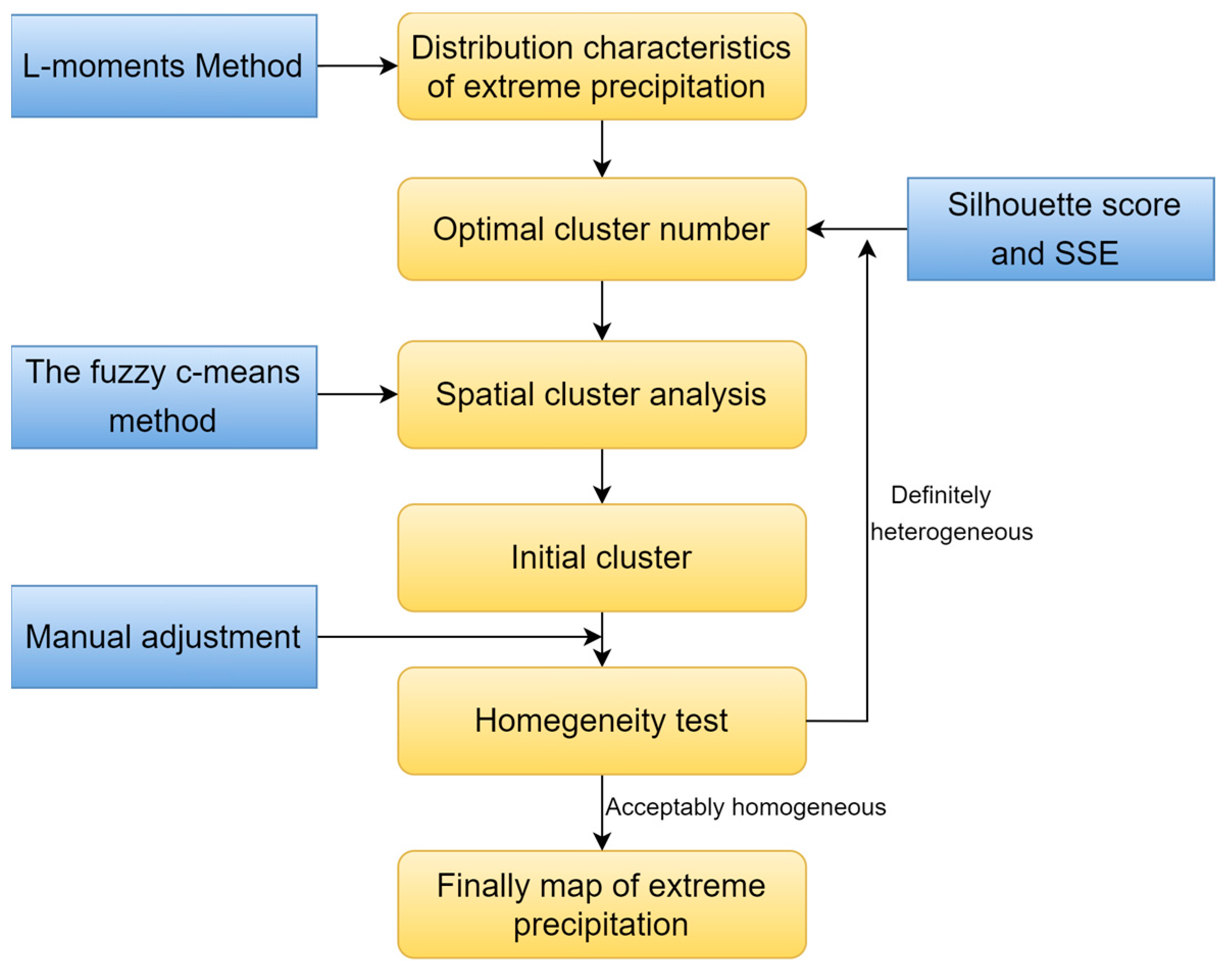
2. Materials and Methods

2.1. Rain Gauge Data

We chose annual maximum 1–day precipitation and annual maximum 5–day precipitation, which are widely used in the design of infrastructure, to represent the regional extreme precipitation pattern. The daily rain gauge data used in this study were obtained from the Meteorological Science Knowledge Service System from 1961 to 2021, covering 839 weather stations. Considering data continuity and quality, we screened 649 stations with complete daily precipitation records from 1961 to 2017 (Figure 1). The longitude, latitude, and elevation of each station were selected as the geographic information for clustering.

2.2. Methods

Extreme precipitation data were clustered by their statistical characteristics including dispersion degree, asymmetry, and steepness, and geographic information, the station’s longitude, latitude, and elevation (

Table 1. Clustering input information.

Clustering Input Information		Relative Weight
	Averaged annual maximum daily precipitation	1
Dispersion Degree	L–CV	0.33
Asymmetry	L–skewness	0.33
Steepness	L–kurtosis	0.33
Geographic Information	Elevation	0.5
	Longitude	1
	Latitude	1

). The possible best cluster numbers were obtained by the Silhouette score and SSE methods. Cluster analysis was used to obtain the initial clusters, which were then manually adjusted to detect homogeneity. The clustering result with the highest homogeneity detection was then chosen. The main procedure is sketched in Figure 2.

2.2.1. L–Moments Method and Data Preprocessing

The variance, skewness, and kurtosis of extreme precipitation series were calculated by the L–moments method introduced by [29]. The L–moment framework has been widely applied in RFA after cluster analysis to estimate the frequency of extreme precipitation [17,20,21,30,31], and we applied it to extract information of the extreme precipitation characteristics. The method is robust in terms of sampling variability by the probability–weighted moment (PWM), which is defined as

$${\alpha }_r={\int }_0^1{z\left(F\right)F\left(z\right)}^{r}dF,r=0,1,2,\dots$$

(1)

The first four L–moments, expressed as linear combinations of PWMs, were computed by using the following relationships:

$$\begin{array}{cc}{\lambda }_1& ={\alpha }_0\hfill \\ {\lambda }_2& ={2\alpha }_1-{\alpha }_0\hfill \\ {\lambda }_3& ={6\alpha }_2-{6\alpha }_1+{\alpha }_0\hfill \\ {\lambda }_4& ={20\alpha }_3-{30\alpha }_2+{12\alpha }_1-{\alpha }_0\hfill \end{array}$$

(2)

The variance, skewness, and kurtosis of the distribution of extreme precipitation by the L–coefficients of variation (L–CV, τ), L–skewness (${\tau }_3$), and L–kurtosis (${\tau }_4$), were computed as $\tau ={\lambda }_2/{\lambda }_1$, ${\tau }_3={\lambda }_3/{\lambda }_2$, and ${\tau }_4={\lambda }_4/{\lambda }_3$ respectively. We normalized all the data and details of the preprocessed data are shown in Table 1. The weightage assigned to the annual average maximum rainfall was 1 in this research paper. Furthermore, a weight of 0.33 was assigned to each of the other three precipitation characteristics (variance, skewness, and kurtosis). The geographic information’s longitude and latitude information were assigned a weight of 1, while the elevation was assigned a weight of 0.5.

2.2.2. Fuzzy C–Means (FCM) Cluster Analysis

Dunn et al. (1973) initially proposed the concept of Fuzzy C–mean cluster analysis [32], and in recent years, with the continuous development of computer science, this method has been further refined and utilized in the field of hydrology [17,33]. The main idea of FCM is to minimize the sum of Euclidean distances from each point to all cluster centers. The objective function of FCM, which is the Euclidean distance from each point to all cluster centers, can be expressed as

$$J_m=\sum _{i=1}^N\sum _{j=1}^C{u}_{ij}^m{\left|\right|x_i-c_j\left|\right|}^2,1\le m<\infty$$

(3)

where m is the membership factor (any real number greater than 1, and we set it as 2 in this study), $x_i$ is the i–th d–dimensional measured site data, $c_j$ is the d–dimension center of the cluster, $u_{ij}$ is the degree of membership of $x_i$ in cluster j, and ||*|| is any norm to express the similarity between any measured data and the center. According to the iterative relationship between $u_{ij}$ and $c_j$,

$$u_{ij}=\frac{1}{\sum _{k=1}^c{\left(\frac{\left|\left|x_i-c_j\right|\right|}{\left|\left|x_i-c_k\right|\right|}\right)}^{\frac{2}{m-1}}}$$

(4)

$$c_j=\frac{\sum _{i=1}^N{u}_{ij}^m\times x_i}{\sum _{i=1}^N{u}_{ij}^m}$$

(5)

We minimized the objective function to get the best $c_j$ and $u_{ij}$ based on a set of randomly generated initial $u_{ij}$.

Before clustering, the best cluster number of $c_j$ should be determined, which we determined by calculating the sum–of–squared error (SSE), which is the sum of squares of distance errors between the points in the cluster and the central point, and the Silhouette score (S) which is an indicator describing the sharpness of the profile of each cluster after clustering.

$$SSE=\sum _{j=1}^C\sum _{i=1}^N{|x_i-c_j|}^2$$

(6)

where $x_i$ is the sample point and $c_j$ is the center of the i–th cluster. As the number of clusters increases, the aggregation within the clusters increases and the sum of squared errors decreases. Therefore, the inflection point of the SSE–cluster number line corresponds to the optimal number of clusters.

$$S=\sum s\left(i\right)=\sum \frac{b\left(i\right)-a\left(i\right)}{max\left(b\left(i\right),a\left(i\right)\right)}$$

(7)

where $a\left(i\right)=\frac{1}{n-1}\sum diatance\left(i,j\right)$, shows the aggregation within its cluster, and $b\left(i\right)$ shows the distance between the point and other clusters, which is calculated in a similar way to $a\left(i\right)$. The value of S is between (−1, 1); the larger the S, the better the clustering.

Therefore, the selection criterion was that as the number of clusters increased, when SSE tended to be stable, clusters with larger S were better. In addition, we used fewer regions to summarize the regional characteristics of extreme precipitation. Combining these considerations, we selected cluster numbers for 1–day and 5–day durations, respectively, and determined the final number of clusters based on their homogeneity performance. It is worth noting that the number of clusters may not be the final number of regions because some adjustments should be made after clustering [17,28,34].

2.2.3. Homogeneity Test

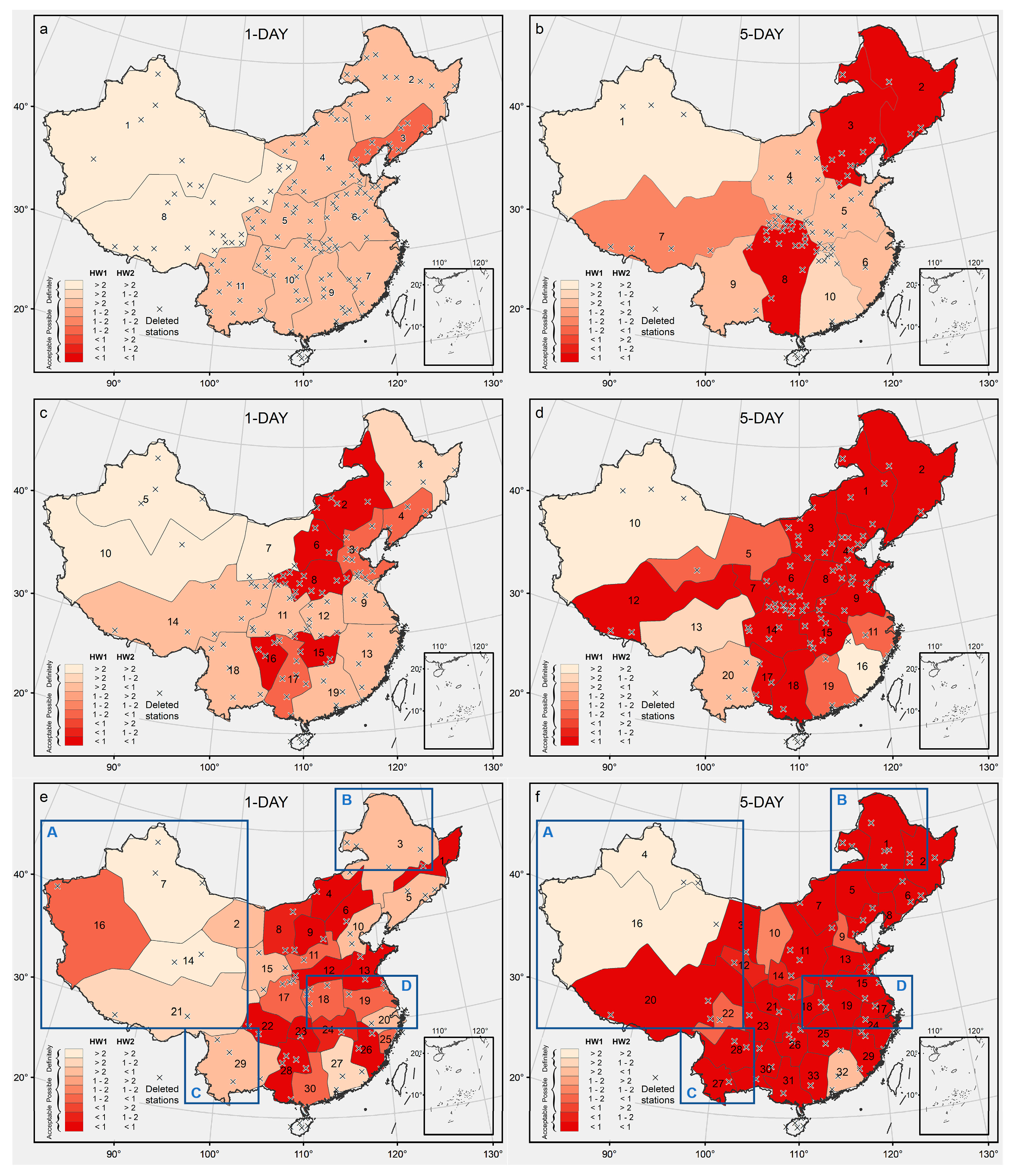
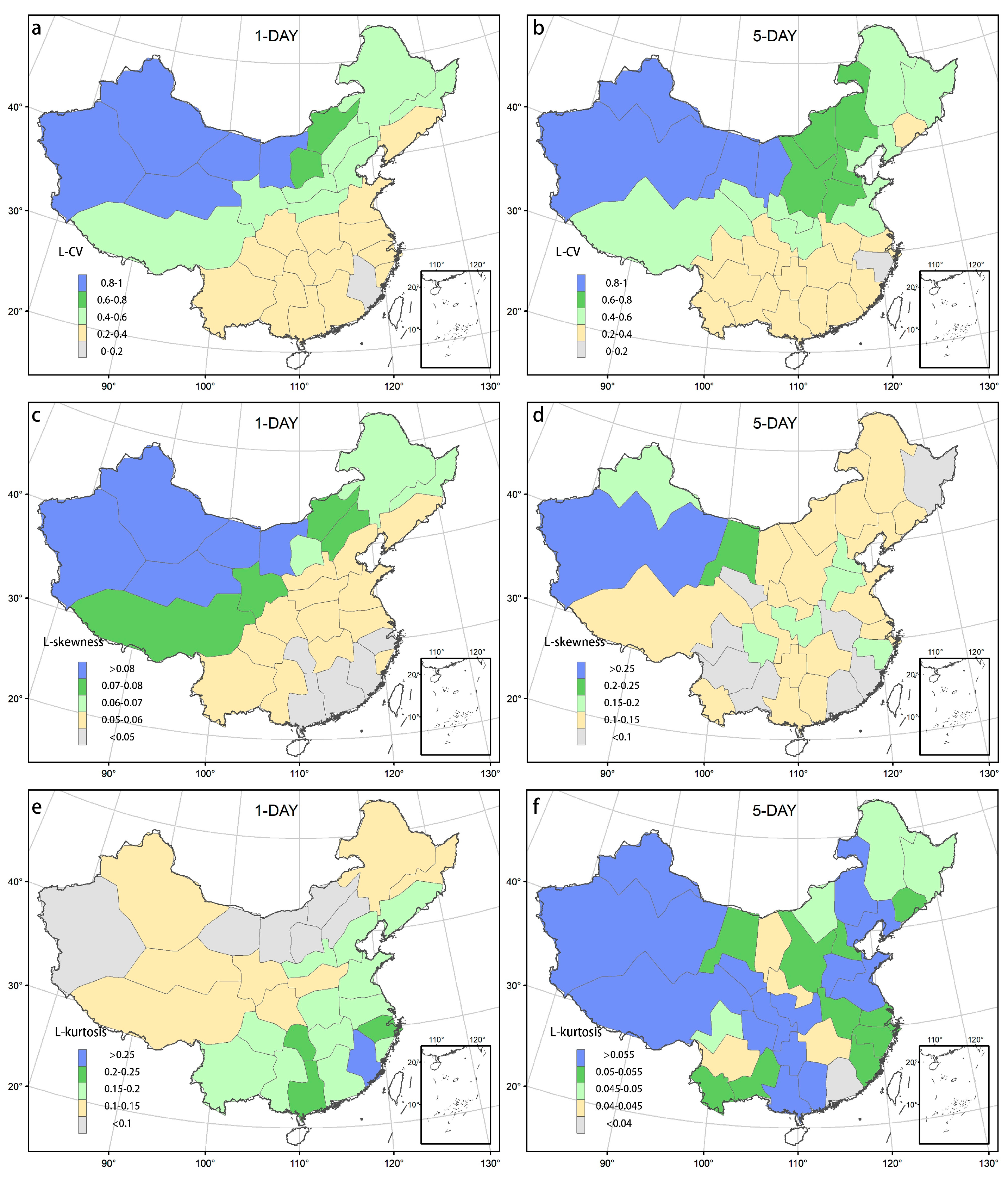
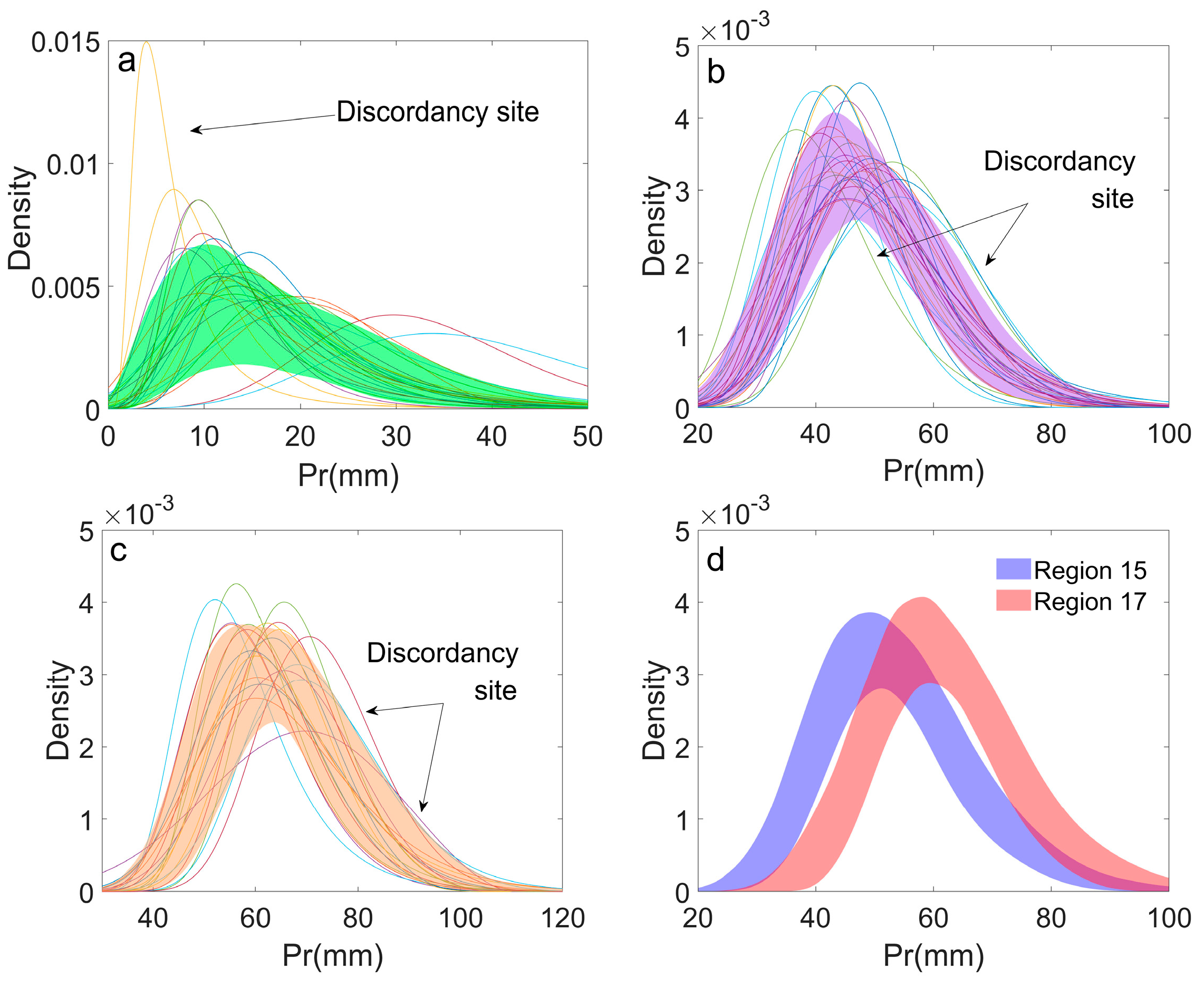
It is necessary to identify the discordancy sites in the region before the homogeneity test. Based on L–moments, the discordancy measure ($D_i$) was defined by

$$D_i=\frac{1}{3}N{\left({\mu }_i-\overline{\mu }\right)}^T{A}^{-1}\left({\mu }_i-\overline{\mu }\right),i=1,2,\dots ,N$$

(8)

where N is the site number of the region, ${\mu }_i=\left[{\tau }^i{\tau }_3^i{\tau }_4^i\right]$, $\overline{\mu }=\left[\overline{\tau }\overline{{\tau }_3}\overline{{\tau }_4}\right]$, and $A=\sum _{i=1}^N\left({\mu }_i-\overline{\mu }\right){\left({\mu }_i-\overline{\mu }\right)}^T$. For site i, if its $D_i$ is greater than the critical value, it is considered a discordant site, while critical values are based on Hosking et al. (1997) according to different N values [34]. The homogeneity test was used to test the homogeneity of the region, which is defined as

$$H=\frac{\left(V-{\delta }_v\right)}{{\sigma }_V}$$

(9)

where $V$ is the weighted standard deviation of at–site sample coefficients of L–variation, which was obtained through simulation by the R software package. Following Norbiato et al. (2007) and Yang et al. (2010), $H_1$ and $H_2$ were used as the homogeneity critical, while Hosking et al. (1997) indicated that $H_2$ was weaker than $H_1$ [18,34,35]. Therefore, $H_1$ was taken as the dominant factor and $H_2$ as the cofactor of $H_1$ to evaluate homogeneity, and we defined the region as “acceptably homogeneous” when $H_1$ < 1 and $H_2$ < 2, as “definitely heterogeneous” when $H_1$ > 2 and $H_2$ > 1, and as “possibly heterogeneous” for other conditions.

3. Results

3.1. Conventional Climate Regions of China

We tested the homogeneity of extreme precipitation for the conventional climate regions in Figure 3. Overall, the conventional climate regions showed poor homogeneity for both 1–day and 5–day durations, with only 9.68% and 29.91% areas being “acceptably homogeneous” regions, respectively. It suggests that the conventional mapping failed to categorize the extreme precipitation patterns. For 1 day, the sub–regions of the North Temperate Zone (IIIB1 and IIIB2) and the IIC1 of the Middle Temperate Zone, mainly in North China, were “acceptably homogeneous”. The performance of the 5–day map was relatively better, with “acceptably homogeneous” areas expanded mainly in North and South China, including eight sub–regions of the Middle Temperate Zone and Central Subtropical Zone. It was noted that for both 1–day and 5–day extreme precipitation maps (Figure 3b,c), there existed many discordancy sites (143 for 1 day and 144 for 5–day precipitation), which suggested poor performance of the conventional climate map to summarize extreme precipitation patterns and led to the failure of the homogeneity test in some regions, especially in the Plateau Climate zone (all sub–regions except for HA1). We framed four areas with poor homogeneity in the conventional climate maps that need to be improved: most of the northwest (A), parts of the southwest (C), parts of the northeast (B), and the middle and lower reaches of the Yangtze River basin in the south (D), and we focused on the performance of our division in these areas.

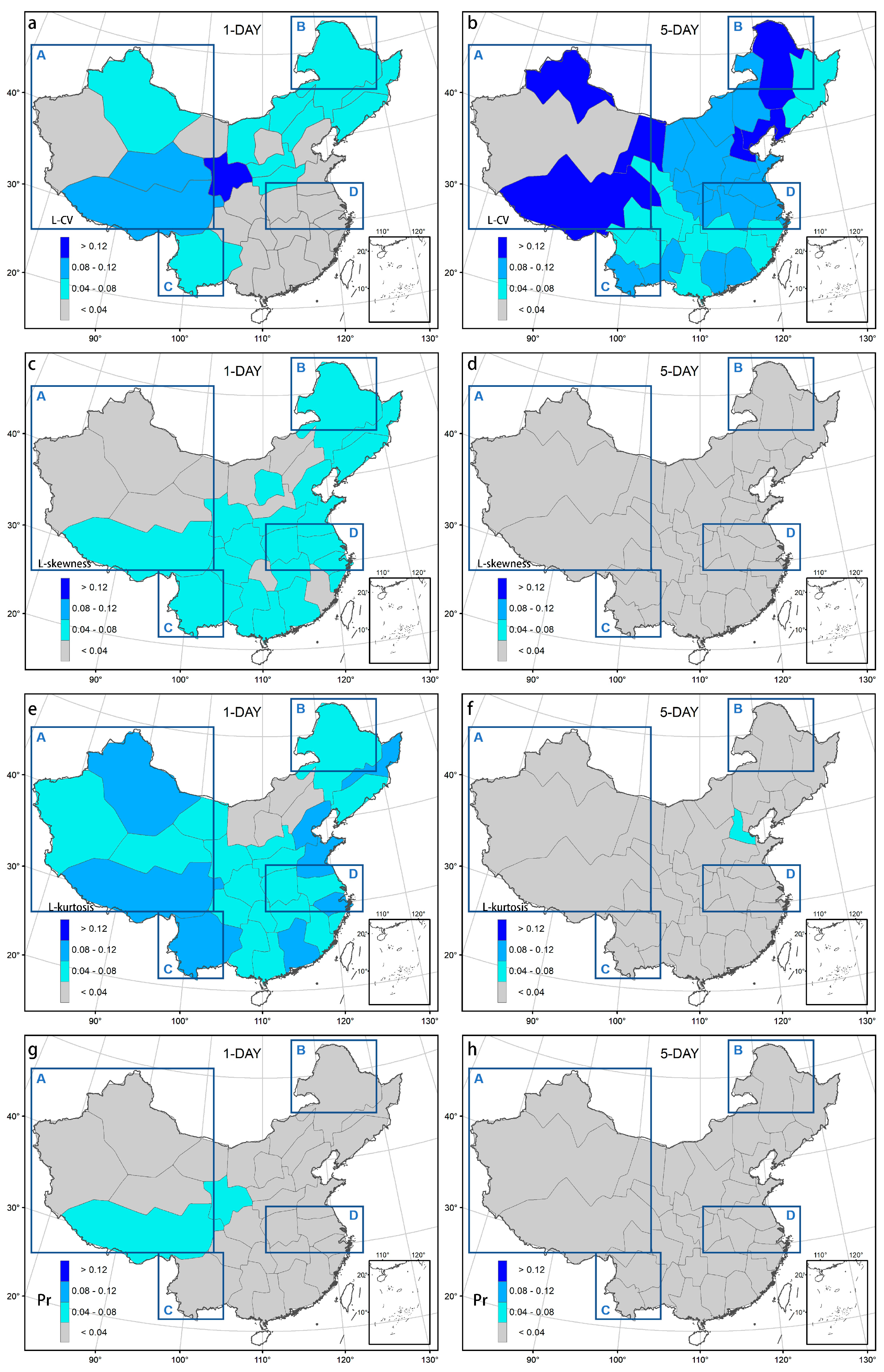
3.2. Clustering Based on Extreme Precipitation Characteristics

We classified into three levels (11, 19, and 30 regions for 1 day, and 10, 20, and 33 regions for 5 days) as shown in Figure 4. It was not surprising that the homogeneity became significantly better with more divisions. For the 1–day map, the “acceptable” homogeneity areas were 0, 14.55%, and 21.54%, and the numbers of discordancy sites were 155, 115, and 79 for Figure 4a,c,e, respectively. For the 5–day map, the “acceptable” homogeneity areas were 27.00%, 50.50%, and 66.85%, and the numbers of discordancy sites were 88, 91, and 75 for Figure 4b,d,f, respectively. Both increased by about 120% compared to the conventional climate zoning.

Comparing Figure 4e,f with Figure 3, which have close region numbers, our division showed significant differences from the conventional maps. Our division showed fewer western regions but denser eastern regions than conventional climate regions. Specifically, 14 sub–regions of western China in Figure 3 were reintegrated and divided into 2–6 regions in all maps of Figure 4. It suggested that the precipitation characteristics in this region were comparatively consistent, or that the limited number of stations available hindered the ability to detect more extreme precipitation features. Further, there was also a significant difference in the region boundaries.

In the conventional climate maps, both the first–level climate zones and the sub–regions were mainly distributed in east–west strips, while our division boundaries were irregular and blocky. It implied that our method better detected the boundaries of extreme precipitation characteristics. Furthermore, our division significantly improved the clustering in the B, C, and D areas. For 1–day extreme precipitation, our map had improved from being “definitely heterogeneous” to “possibly heterogeneous” compared to the conventional map in B, C, and D, while for 5–day extreme precipitation, the improvement of our map had been from “definitely heterogeneous” to “acceptable homogeneous”. The intrinsic differences in characteristics of different rainfall durations may also be an important cause that cannot be ignored and we will further analyze this in the Discussion section.

Having achieved a higher level of homogeneity, we further investigated the extreme precipitation characteristics of various regions in China (Figure 5). In the western and northern regions, the L–CV and L–skewness values of extreme precipitation were significantly higher, which suggested that in these regions, the amount of extreme precipitation varied drastically and was subject to sudden and intense episodes of extreme precipitation. The L–kurtosis value of 1–day precipitation decreased from southeast to northwest, which was consistent with the pattern of extreme precipitation in southeastern China being more frequent and intense. However, this pattern was not reflected in the 5–day extreme precipitation, with very high L–kurtosis values observed in certain regions of western, northern, and southern China, suggesting that long–term extreme precipitation may have distinct distribution characteristics compared to short–term extreme precipitation. Additionally, there existed certain regions exhibited distinctive precipitation features. For example, in the northeast, 1–day extreme precipitation showed high L–CV, high L–skewness, and low L–kurtosis, which was consistent with most areas of the southeast to the northwest of China, while 5–day extreme precipitation showed high L–CV, low L–skewness, and high L–kurtosis, implying a lower threat of long duration extreme precipitation. The Pearl River basin in southern China showed low L–CV and L–skewness overall, but its upper reaches showed high L–kurtosis and low L–kurtosis downstream, meaning that the upper reaches may face a heightened risk of extreme precipitation.

Unfortunately, our map also showed poor homogeneity in most of the regions in northwest China (region A), although it was only divided into 4–6 regions to ensure homogeneity testing. The reason may be attributed to the high variance of extreme precipitation. For example, in region 16 of Figure 4f, although we removed the discordancy site, the shapes and positions of their probability distribution curves were too scattered to be considered as the same extreme precipitation pattern (Figure 6a). It implies that these sites were grouped into a cluster only because of similar geographical features rather than extreme precipitation characteristics. By comparison, the curves of all sites in the region were gathered in a small range in some regions of B, C, and D (Figure 6b–d) with excellent homogeneity. Furthermore, we plotted the pdfs of all sites in regions 15 and 17 of Figure 4f, belonging to the same sub–region in the conventional map (IVA1), to test the performance of distinguishing different extreme precipitation patterns of our map. We noticed a clear difference between the two clusters of curves. Region 15 showed a greater variance but a smaller value of extreme precipitation (about 45 mm), while region 17 showed smaller variance but greater values of extreme precipitation (about 60 mm). It suggested different precipitation patterns in geographically adjacent areas, and our map effectively identified this difference where the conventional map failed.

4. Discussion

We also made a comparison with the method of Wang et al. (2017) [17]. Overall, the shape distribution and homogeneity characteristics were consistent with ours in Figure 4, which showed the characteristics of fewer western regions but denser eastern regions and irregular block distribution. However, our division had better homogeneity than Wang et al. (2017) (Figure 7) [17]. The homogeneity regions of Figure 7a,b covered only 17.66% and 47.34% areas, respectively, which were significantly less than Figure 4e,f (21.54% and 66.85%). Furthermore, we noticed that more “acceptably homogeneous” could be found in Figure 4e than in Figure 7a. Compared with Figure 7a the advantages of our map for short precipitation duration (1 day) were mainly reflected in northern China, while in some regions of eastern China, our map was disadvantaged. For longer precipitation duration (5 days), our map performed significantly better, and the advantageous areas were mainly distributed in southwestern and eastern China (regions B, C, and D). Overall, the result suggested that using the distribution characteristics of extreme precipitation by cluster analysis benefitted a lot in summarizing regional extreme precipitation patterns.

Results showed that the homogeneity of 1–day extreme precipitation was always worse than that of 5 days, though the number of regions was close. To find the reason, we calculated the differences between sites in the region of mean annual maximum precipitation, L–CV, L–skewness, and L–kurtosis in each region of Figure 4e,f after normalization. As shown in Figure 8, except for L–CV, the differences between sites in the region of mean annual maximum precipitation, L–skewness, and L–kurtosis for 1 day were significantly higher than those for 5–day precipitation for most regions, which implied less regularity in 1–day maps. Regions B, C, and D exhibited lower standard deviation in L–CV, L–skewness, and L–kurtosis, signifying an improved homogeneity of 5–day extreme precipitation. It is known that a higher standard deviation means a more significant difference among the sites in this region.

For details, we selected some sites in regions B, C, and D, to show their different shapes in the pdf of 1 day and 5 days (Figure 9). Although these sites roughly overlapped, curves of 1 day showed more significant variations than did 5–day curves. We noticed that both kurtosis and location of the distribution curves of 1–day extreme precipitation showed significant differences, and curves with higher precipitation values corresponding to peak locations had steeper peaks. This result suggested two different patterns of extreme precipitation: a smaller mean with a larger variance, and a larger mean with smaller variance. It explained the better homogeneity of the 5–day extreme precipitation and the difficulty of summarizing regional patterns of 1–day extreme precipitation characteristics of geographically closed sites. Some studies have also indicated the necessity for analysis of extreme regional precipitation with varying durations, including the distribution curves and nonstationary change trends [36,37]. It implies the necessity of further analysis of the differences in durations of extreme precipitation.

5. Conclusions

In this paper, we clustered China’s extreme precipitation pattern based on the distribution characteristics of observed precipitation data by L–moment method and cluster analysis using 1–day and 5–day extreme precipitation data. In contrast to the general approach, we attempted to further extract the distribution curve characteristics of extreme precipitation for cluster analysis to better summarize extreme precipitation patterns.

Based on our study, China can be divided into 30–33 regions with different extreme precipitation patterns. As the number of regions increases, the proportion of regions with good homogeneity increases, but the number of stations in each region decreases, resulting in too little data to pass the homogeneity test. After continuous debugging, we found that the regional differences of extreme precipitation in China were better distinguished when the number of regions for 1–day and 5–day durations was 30 and 33, respectively.

Our maps have improved the ability to characterize the spatial distribution of extreme precipitation patterns compared with the conventional climate map, mainly in parts of northeast, southeast, and southwest China. The regions with good homogeneity of 1–day and 5–day extreme precipitation increased about 120% in our map compared with the conventional map. In addition, a comparison of our maps with the results obtained using the method of Wang et al. (2017) showed the necessity of adopting more extreme precipitation information to increase the clustering homogeneity.

In western and northern China, the intensity of extreme precipitation was highly variable and was likely to cause sudden, intense extreme precipitation disasters. In contrast, frequent and persistent high–intensity precipitation was a more pressing concern in southeastern China. Additionally, extreme precipitation characteristics of different durations varied greatly, and extreme precipitation of long duration had more significant spatial distribution regularity. The distribution characteristics of short–duration extreme precipitation (1 day), including L–CV, L–skewness, and L–kurtosis of the distribution curves, showed less spatial distribution regularity than did long–duration (5–day) precipitation. The proportion of regions with high homogeneity of 5–day extreme precipitation was significantly higher than that of 1 day. Therefore, future analysis of extreme regional precipitation should focus on comprehensive consideration of precipitation duration, intensity, frequency, and nonstationary change of extreme precipitation and develop a dynamic division to evaluate the development of extreme precipitation and prevent risks.

References

1. Abbas, A.; Waseem, M.; Ullah, W.; Zhao, C.; Zhu, J. Spatiotemporal analysis of meteorological and hydrological droughts and their propagations. Water 2021, 13, 2237. [Google Scholar] [CrossRef]
2. Dottori, F.; Szewczyk, W.; Ciscar, J.C.; Zhao, F.; Alfieri, L.; Hirabayashi, Y.; Bianchi, A.; Mongelli, I.; Frieler, K.; Betts, R.A.; et al. Increased human and economic losses from river flooding with anthropogenic warming. Nat. Clim. Chang. 2018, 8, 781–786. [Google Scholar] [CrossRef]
3. Elahi, E.; Khalid, Z.; Tauni, M.Z.; Zhang, H.; Lirong, X. Extreme weather events risk to crop-production and the adaptation of innovative management strategies to mitigate the risk: A retrospective survey of rural Punjab, Pakistan. Technovation 2022, 117, 102255. [Google Scholar] [CrossRef]
4. Elahi, E.; Khalid, Z.; Zhang, Z. Understanding farmers’ intention and willingness to install renewable energy technology: A solution to reduce the environmental emissions of agriculture. Appl. Energy 2022, 309, 118459. [Google Scholar] [CrossRef]
5. Jenifer, M.A.; Jha, M.K. Assessment of precipitation trends and its implications in the semi-arid region of Southern India. Environ. Chall. 2021, 5, 100269. [Google Scholar] [CrossRef]
6. Jongman, B. Effective adaptation to rising flood risk COMMENT. Nat. Commun. 2018, 9, 1986. [Google Scholar] [CrossRef]
7. Waseem, M.; Khurshid, T.; Abbas, A.; Ahmad, I.; Javed, Z. Impact of meteorological drought on agriculture production at different scales in Punjab, Pakistan. J. Water Clim. Chang. 2022, 13, 113–124. [Google Scholar] [CrossRef]
8. Cavanaugh, N.R.; Gershunov, A.; Panorska, A.K.; Kozubowski, T.J. The probability distribution of intense daily precipitation. Geophys. Res. Lett. 2015, 42, 1560–1567. [Google Scholar] [CrossRef]
9. Gentilucci, M.; Barbieri, M.; Pambianchi, G. Reliability of the IMERG product through reference rain gauges in Central Italy. Atmos. Res. 2022, 278, 106340. [Google Scholar] [CrossRef]
10. Huang, H.; Cui, H.; Ge, Q. Assessment of potential risks induced by increasing extreme precipitation under climate change. Nat. Hazards 2021, 108, 2059–2079. [Google Scholar] [CrossRef]
11. Huang, H.; Cui, H.; Ge, Q. Will a nonstationary change in extreme precipitation affect dam security in China? J. Hydrol. 2021, 603, 126859. [Google Scholar] [CrossRef]
12. Papalexiou, S.M.; Montanari, A. Global and Regional Increase of Precipitation Extremes Under Global Warming. Water Resour. Res. 2019, 55, 4901–4914. [Google Scholar] [CrossRef]
13. Trenberth, K.E. Changes in precipitation with climate change. Clim. Res. 2011, 47, 123–138. [Google Scholar] [CrossRef]
14. Huang, J.P.; Ran, J.J.; Ji, M.X. Preliminary analysis of the flood disaster over the arid and semi-arid regions in China. Acta Meteorol. Sin. 2014, 72, 1096–1107. [Google Scholar]
15. Zheng, W.W.; Yang, Y.D.; Man, Z.M. Multiple movement characteristics of the Meiyu rain belt in East Asia: Reconstructing historical data on the southern margin from 1861 to 2017. Clim. Chang. 2021, 165, 20. [Google Scholar]
16. Abdi, A.; Hassanzadeh, Y.; Ouarda, T.B. Regional frequency analysis using Growing Neural Gas network. J. Hydrol. 2017, 550, 92–102. [Google Scholar] [CrossRef]
17. Wang, Z.L.; Zeng, Z.Y.; Lai, C.G.; Lin, W.X.; Wu, X.S.; Chen, X.H. A regional frequency analysis of precipitation extremes in Mainland China with fuzzy c-means and L-moments approaches. Int. J. Climatol. 2017, 37, 429–444. [Google Scholar] [CrossRef]
18. Yang, T.; Shao, Q.X.; Hao, Z.C.; Chen, X.; Zhang, Z.X.; Xu, C.Y.; Sun, L.M. Regional frequency analysis and spatio-temporal pattern characterization of rainfall extremes in the Pearl River Basin, China. J. Hydrol. 2010, 380, 386–405. [Google Scholar] [CrossRef]
19. Darwish, M.M.; Tye, M.R.; Prein, A.F.; Fowler, H.J.; Blenkinsop, S.; Dale, M.; Faulkner, D. New hourly extreme precipitation regions and regional annual probability estimates for the UK. Int. J. Climatol. 2021, 41, 582–600. [Google Scholar] [CrossRef]
20. Liu, J.; Doan, C.D.; Liong, S.-Y.; Sanders, R.; Dao, A.T.; Fewtrell, T. Regional frequency analysis of extreme rainfall events in Jakarta. Nat. Hazards 2015, 75, 1075–1104. [Google Scholar] [CrossRef]
21. Zakaria, Z.A.; Shabri, A.; Ahmad, U.N. Regional Frequency Analysis of Extreme Rainfalls in the West Coast of Peninsular Malaysia using Partial L-Moments. Water Resour. Manag. 2012, 26, 4417–4433. [Google Scholar] [CrossRef]
22. Rajsekhar, D.; Mishra, A.K.; Singh, V.P. Regionalization of Drought Characteristics Using an Entropy Approach. J. Hydrol. Eng. 2013, 18, 870–887. [Google Scholar] [CrossRef]
23. Zhuang, W.Y.; Ding, W. Long-lead prediction of extreme precipitation cluster via a spatiotemporal convolutional neural network. In Proceedings of the 6th International Workshop on Climate Informatics (CI 2016), San Francisco, CA, USA, 13–17 August 2016. [Google Scholar]
24. Zhang, B.K.; Zhu, G.K. The Climate Regionalization in China; China Science Publishing: Beijing, China, 1959; pp. 1–297. [Google Scholar]
25. Amini, S.; Straus, D.M. Control of Storminess over the Pacific and North America by Circulation Regimes: The role of large-scale dynamics in weather extremes. Clim. Dyn. 2019, 52, 4749–4770. [Google Scholar] [CrossRef]
26. Horton, D.E.; Johnson, N.C.; Singh, D.; Swain, D.L.; Rajaratnam, B.; Diffenbaugh, N.S. Contribution of changes in atmospheric circulation patterns to extreme temperature trends. Nature 2015, 522, 465–469. [Google Scholar] [CrossRef]
27. Zhang, Q.; Qi, T.Y.; Singh, V.P.; Chen, Y.D.; Xiao, M.Z. Regional Frequency Analysis of Droughts in China: A Multivariate Perspective. Water Resour. Manag. 2015, 29, 1767–1787. [Google Scholar] [CrossRef]
28. Chen, Y.D.; Zhang, Q.; Xiao, M.Z.; Singh, V.P.; Leung, Y.; Jiang, L.G. Precipitation extremes in the Yangtze River Basin, China: Regional frequency and spatial-temporal patterns. Theor. Appl. Climatol. 2014, 116, 447–461. [Google Scholar] [CrossRef]
29. Hosking, J.R.M. L-Moments: Analysis and Estimation of Distributions Using Linear Combinations of Order Statistics. J. R. Stat. Soc. Ser. B 1990, 52, 105–124. [Google Scholar] [CrossRef]
30. Fowler, H.J.; Kilsby, C.G. A regional frequency analysis of United Kingdom extreme rainfall from 1961 to 2000. Int. J. Clim. 2003, 23, 1313–1334. [Google Scholar] [CrossRef]
31. Gaál, L.; Kyselý, J.; Szolgay, J. Region-of-influence approach to a frequency analysis of heavy precipitation in Slovakia. Hydrol. Earth Syst. Sci. 2008, 12, 825–839. [Google Scholar] [CrossRef]
32. Dunn, J.C. A fuzzy relative of the ISODATA Process and Its Use in Detecting Compact Well-Separated Clusters. J. Cybern. 1973, 3, 32–57. [Google Scholar] [CrossRef]
33. Askari, S. Fuzzy C-Means clustering algorithm for data with unequal cluster sizes and contaminated with noise and outliers: Review and development. Expert Syst. Appl. 2021, 165, 113856. [Google Scholar] [CrossRef]
34. Hosking, J.R.M.; Wallis, J.R. Regional frequency analysis: An approach based on L-moments. J. Am. Stat. Assoc. 1997, 93, 1233. [Google Scholar]
35. Norbiato, D.; Borga, M.; Sangati, M.; Zanon, F. Regional frequency analysis of extreme precipitation in the eastern Italian Alps and the August 29, 2003 flash flood. J. Hydrol. 2007, 345, 149–166. [Google Scholar] [CrossRef]
36. Du, H.B.; Alexander, L.V.; Donat, M.G.; Lippmann, T.; Srivastava, A.; Salinger, J.; Kruger, A.; Choi, G.; He, H.S.; Fujibe, F.; et al. Precipitation From Persistent Extremes is Increasing in Most Regions and Globally. Geophys. Res. Lett. 2019, 46, 6041–6049. [Google Scholar] [CrossRef]
37. Dwyer, J.G.; O’Gorman, P.A. Changing duration and spatial extent of midlatitude precipitation extremes across different climates. Geophys. Res. Lett. 2017, 44, 5863–5871. [Google Scholar] [CrossRef]
Figure 1. Distribution of 649 stations and mean annual maximum 1–day (a) and 5–day (b) precipitation.
Water 15 03651 g001
Figure 2. Calculation flowchart.
Water 15 03651 g002
Figure 3. (a) Conventional climate regions of China and (b) the homogeneity of 1–day and (c) 5–day extreme precipitation.
Water 15 03651 g003
Figure 4. Final regions for 1 day (a,c,e) and 5 days (b,d,f) based on extreme precipitation characteristics within three stages.
Water 15 03651 g004
Figure 5. The mean value of normalized L–CV (a,b), L–skewness (c,d), and L–kurtosis (e,f) for the division of Figure 4e,f for 1 day and 5 days.
Water 15 03651 g005
Figure 6. Probability density curve of all sites and their distribution range in (a) region 16 of Figure 4f, (b) region 1 of Figure 4f, and (c) region 30 of Figure 4f. The distribution range of the probability density curve of all sites in (d) regions 15 and 17 of Figure 4f.
Water 15 03651 g006
Figure 7. Final regions for (a) 1–day and (b) 5–day extreme precipitation characteristics based on the method of Wang et al. (2017) [17].
Water 15 03651 g007
Figure 8. The standard deviation of the normalized mean maximum precipitation (g,h), L–CV (a,b), L–skewness (c,d), and L–kurtosis (e,f) for the division of Figure 4e,f for 1–day and 5–day extreme precipitation characteristics.
Water 15 03651 g008
Figure 9. The distribution range of the probability density curve of (a) region 3 of Figure 4e and region 1 of Figure 4f in B; (b) region 28 of Figure 4f and region 29 of Figure 4e in C; and (c) region 19 of Figure 4f and region 15 of Figure 4e.
Water 15 03651 g009