Article

A Non-Stationarity Analysis of Annual Maximum Floods: A Case Study of Campaspe River Basin, Australia

1
Department of Engineering, La Trobe University, Melbourne 3086, Australia
2
Department of Civil and Construction Engineering, Swinburne University of Technology, Melbourne 3122, Australia
3
Civil and Environmental Engineering Department, University of Sharjah, Sharjah P.O. Box 27272, United Arab Emirates
4
Department of Civil Engineering, American University of Sharjah, Sharjah P.O. Box 26666, United Arab Emirates
5
School of Engineering, Design and Built Environment, Western Sydney University, Sydney 1797, Australia
*
Author to whom correspondence should be addressed.
Water 2023, 15(20), 3683; https://doi.org/10.3390/w15203683
Submission received: 13 September 2023 / Revised: 16 October 2023 / Accepted: 17 October 2023 / Published: 21 October 2023
(This article belongs to the Special Issue Flood Frequency Analysis and Modelling)

Abstract

:
A design flood is an essential input for water infrastructure design and flood protection. A flood frequency analysis has been traditionally performed under stationarity assumption indicating that the statistical properties of historical flooding will not change over time. Climate change and variability challenges the stationarity assumption, and a flood frequency analysis without consideration of non-stationarity can result in under- or overestimation of the design floods. In this study, non-stationarity of annual maximum floods (AMFs) was investigated through a methodology consisting of trend and change point tests, and non-stationary Generalized Extreme Value (NSGEV) models, and the methodology was applied to Campaspe River Basin as a case study. Statistically significant decreasing trends in AMFs were detected for almost all stations at the 0.01 significance level in Campaspe River Basin. NSGEV models outperformed the stationary counterparts (SGEV) for some stations based on statistical methods (i.e., Akaike information criterion (AIC) and Bayesian information criterion (BIC)) and graphical approaches (i.e., probability and quantile plots). For example, at Station 406235, AIC and BIC values were found to be 334 and 339, respectively, for the SGEV model, whereas AIC and BIC values were calculated as 330 and 334, respectively, for the NSGEV 15 model with time-varying location and scale parameters. Deriving a design flood from conventional stationary models will result in uneconomical water infrastructure design and poor water resource planning and management in the study basin.

1. Introduction

Floods are among the most common and costliest natural disasters worldwide. Accurate estimation of flood magnitudes corresponding to return periods of interest (design flood) is a cornerstone of flood risk management [1]. A design flood is an essential input for water infrastructure design and flood protection. The most direct approach to derive the design flood is to conduct an at-site flood frequency analysis [2].
A flood frequency analysis has been traditionally performed under stationarity assumptions indicating that the statistical properties of historical flooding (or its drivers such as rainfall) will not change over time [3,4]. Climate change and variability challenges the stationarity assumption. Several studies (e.g., [5,6,7]) explained that basic concepts in a flood frequency analysis including probability of exceedance and return period are not valid when non-stationarity exists. The flood frequency analysis without consideration of non-stationarity can result in under- or overestimation of the design floods.
There are several studies that conducted a non-stationary flood frequency analysis in the literature. For example, Šraj et al. [8] employed stationary and non-stationary Generalized Extreme Value (GEV) models using data from two flow stations in Slovenia. They found that the flood quantile estimates from stationary models are lower than those from the non-stationary models in recent years. Ray and Goel [9] examined a stationary and non-stationary flood frequency analysis using annual maximum flood (AMF) data from six gauging sites in Narmada River Basin. They considered both time and physical covariates to develop non-stationary models and reported a significant increase in design floods over time. Chen et al. [1] reported that non-stationary models at several stations overperformed the stationary models in the UK, particularly the ones with rainfall-related covariates. Singh and Chinnasamy [10] developed stationary and non-stationary GEV models to perform a flood frequency analysis for Periyar River and found that using stationary models instead of optimal non-stationary models may result in unsafe design of the structure. Hounkpè et al. [11] developed time- and/or physical-covariate-dependent GEV models for a frequency analysis using AMF data from five flow stations in the Ouémé River Basin, Benin Republic. They reported that a non-stationary model with a linear trend in its location parameter showed the best performance and sufficiently explained the variation in the data. Bossa et al. [12] developed both stationary and non-stationary GEV models using AMF data and sea surface temperature (as a climate index covariate) across stations spread over West Africa. It was found in this study that non-stationary GEV models outperform stationary models for majority of the stations. Anzolin et al. [13] studied stationary and non-stationary GEV models for an AMF frequency analysis using five covariates (for the non-stationary models), including annual temperature, El Nino Southern Oscillation, annual rainfall, annual maximum rainfall, and annual maximum soil moisture content. The authors reported that non-stationary models are preferable for some of the studied stations, and they stated that non-stationary models with rainfall-based covariates showed better performance.
In the literature, there are several Australian studies investigating non-stationarity of AMFs. For example, Ishak et al. [14] employed the Mann–Kendal (MK) test to examine trends in AMFs as the trends may be an indicator of the non-stationarity. Do et al. [15] examined AMF trends globally including data from the east coast of Australia using the Global Runoff Data Centre database. Ishak and Rahman [16] adopted MK and Pettitt change point detection tests to study changes in Australian AMF data. All abovementioned Australian studies reported significant decreasing trends in AMFs in South-East Australia. When non-stationarity is detected in extreme values (i.e., annual maximum rainfall, temperature, or floods), it is recommended to conduct a non-stationary frequency analysis to ensure whether a stationary or non-stationary frequency analysis results in more accurate design value estimations corresponding to different return periods [17]. Although there are several studies on non-stationarity of AMFs, the number of studies performing a non-stationary flood frequency analysis is very limited in Australia. As an example, Han et al. [18] performed a non-stationary regional flood frequency analysis in several Australian catchments and estimated changes in flood quantiles in 2100. They predicted decreases in flood quantiles corresponding to a 2-year (Q2) and 20-year (Q20) return period at the majority of the studied catchments in the state of Victoria (with a more significant decrease in Q20 estimations).
In this study, a generic methodology consisting of non-stationarity detection and a non-stationary flood frequency analysis was applied using data from Campaspe River Basin, located in north-central Victoria. The commonly used non-parametric tests including MK trend and Pettitt change point tests were applied first to detect non-stationarities as performed in several studies (e.g., [19,20]). Then, stationary and non-stationary GEV models were developed for the frequency analysis of AMFs to derive design floods of various return periods. Although there are some AMF trend analysis studies conducted at an Australian scale, most of those studies did not consider all stations in Campaspe River Basin; also, a non-stationary frequency analysis was not applied in those studies. This study aimed to contribute better understanding of the non-stationarity concept in a flood frequency analysis in Australia as well as assisting water engineering practice in Campaspe River Basin through more accurate design flood estimation for safe and cost-effective water infrastructure design and water resource management.

2. Study Area and Data

The Campaspe River Basin with a surface area of 417,914 hectares is located in north-central Victoria. The Campaspe River is a source of domestic, industrial, and commercial water supply, particularly for the Bendigo urban supply area and irrigators in the area between Malmsbury and Bendigo [21]. The length of Campaspe River is around 220 km, and there are four storage reservoirs on the river with Lake Eppalock being the largest with a 304 GL capacity [22].
Quality-controlled AMF data derived from daily streamflow data of six stations, which are located at the outlet of six unregulated sub-basins of Campaspe River Basin, were used for the analysis in this study. As the length of data record is significant for the trend and frequency analysis, stations with a minimum data length of 40 years were considered. Data were derived from hydrologic reference stations [23] created by Bureau of Meteorology, Australia. Location, name, sub-basin area, and available data period of the selected stations are shown in Table 1. Sub-basins with a minimal effect of land-use change and regulation through artificial storage were considered in selection of the stations. The location of the Campaspe River Basin and selected stations are shown in Figure 1.

3. Methodology

The methodology of this study consists of three parts as shown below:
(1)
The AMF trend analysis using the MK test.
(2)
The AMF change point analysis using the Pettitt test.
(3)
The stationary and non-stationary flood frequency analysis.

3.1. AMF Trend Analysis Using MK Test

The MK test was selected for the trend analysis in this study since it is a widely adopted monotonic trend test for a hydro-meteorological time series data analysis (e.g., [24,25]). The MK is a non-parametric test without any assumption about the statistical distribution of the data. This makes the MK test a suitable approach for a trend analysis of non-normally distributed data, which is very common in hydro-meteorology. A positive MK test score (z-score) indicates an increasing trend, whereas a decreasing trend is represented by a negative MK test score. If the calculated test statistic is larger than the critical value at any significance level (e.g., 0.1, 0.05, 0.01), the null hypothesis of no trend is rejected and the detected trend is considered as statistically significant at the same significance level. Critical values at 0.1, 0.05, and 0.01 significance levels are 1.645, 1.96, and 2.576, respectively [26,27,28]. Formulation and details of the MK test can be seen from Kundzewicz and Robson [29].
Data independence is a requirement of the MK test. Autocorrelation plots, produced through computing autocorrelations for data values at a range of time lags, were used to check data independence in this study. In the autocorrelation plots, the lag-n autocorrelation shows the correlation between values in the time series and their preceding value n water years before. For example, lag-1 autocorrelation shows the correlation between values and the value 1 year before. The autocorrelation function at lag-0 is always 1. Autocorrelation estimates can be considered statistically significant at a 0.05 (5%) significance level if the estimates are outside the 95% confidence intervals on the autocorrelation plots.

3.2. AMF Change Point Analysis Using Pettitt Test

The Pettitt test is commonly used for a change point analysis in hydro-meteorological time series data to identify a sudden change in the mean of a time series [30,31]. Shifting time and the significance level are the outputs of the test. Like the MK test, the Pettitt test is a non-parametric technique with no assumption about the data distribution. The null hypothesis of the Pettitt test indicates no difference between the means of the earlier and later portions of time series data. If the test output (p-values) is less than a chosen significance level, then the null hypothesis is rejected, suggesting that there is a sudden change. More detailed information about the Pettitt test can be found from Conte et al. [32].

3.3. Stationary and Non-Stationary Flood Frequency Analysis

3.3.1. Stationary Flood Frequency Analysis

There are two basic methods to derive data for a flood frequency analysis: (1) block maxima, and (2) peaks over threshold (POT). Flood data are produced by selecting the maximum values from each year in the block maxima approach. In this case, flood data are commonly named as AMF. In the POT approach, data above a certain threshold are selected. When there is a sufficient number of data points, the block maxima approach is a suitable approach and serves better for data independency requirements in comparison to the POT approach. In this study, Generalized Extreme Value (GEV) distribution was selected to fit the AMF data for the frequency analysis as recommended and applied by several studies (e.g., [8,10,33]).
The GEV distribution covers the three extreme value distributions including Gumbel, Frechet, and negative Weibull. Equation (1) shows the cumulative distribution function of the GEV distribution.
F x = e x p ( 1 + ξ x μ σ ) 1 / ξ
defined on the set q : 1 + ξ ( q μ ) / σ > 0 , where “μ” represents the location parameter, “σ” corresponds to the scale parameter, and “ξ” is the shape parameter. In case of the shape parameter being equal to zero, the distribution is called Gumbel. The distribution is called Fréchet if the shape parameter is positive, whereas it is named negative Weibull with a negative shape parameter [10,34]. In the stationary GEV models, all three parameters are constant (not dependent on covariates).
Parameters of the GEV models can be estimated through different methods such as the method of moments, the maximum likelihood estimates (MLE), and the L-moments. In this study, the MLE approach was employed since it is a more robust technique [2,35]. The stationary GEV model is abbreviated as SGEV for the rest of the manuscript.

3.3.2. Non-Stationary Flood Frequency Analysis

The parameters of the SGEV model are constant, whereas one or more parameters of non-stationary GEV (NSGEV) models are not fixed. The parameter(s) might change over time or as a response of physical covariates (variable other than flow). The Pacific- and Indian-Ocean-related large-scale climate variabilities including El Niño Southern Oscillation (ENSO), Interdecadal Pacific Oscillation (IPO), Indian Ocean Dipole (IOD), and Southern Annular Mode (SAM) have significant impact on Australian floods [36,37]. Therefore, in this study, indices including the Southern Oscillation Index (SOI), Dipole Mode Index (DMI), Tripole Index (TPI), and SAM index (representing the ENSO, IOD, IPO, and SAM, respectively) were used as physical covariates in NSGEV models in addition to the time covariate.
SOI and TPI data were obtained from the National Oceanic and Atmospheric Administration Physical Sciences Laboratory. SOI data were available from 1856 to 2021 (https://psl.noaa.gov/gcos_wgsp/Timeseries/SOI/ accessed on 5 May 2023), whereas TPI data were derived for the period of 1854–2021 (https://psl.noaa.gov/data/timeseries/IPOTPI/ accessed on 7 May 2023). DIM data, covering the period of 1982–2021, were derived from the Japan Agency for Marine-Earth Science and Technology (https://www.jamstec.go.jp/virtualearth/general/en/index.html accessed on 7 May 2023). SAM index data over the period of 1957–2021 were derived from British Antarctic Survey (https://legacy.bas.ac.uk/met/gjma/sam.html accessed on 10 May 2023). Annual average index values were employed in NSGEV models, and in total 16 GEV models (1 SGEV and 15 NSGEV) were developed for each station in this study. All developed non-stationary models are shown in Table 2.
If the location parameter is varying, the location parameter (μ) is defined based on μ0 and μ1. If the scale parameter shows variation, the ln(scale) parameter (ϕ) is expressed according to ϕ0 and ϕ1, as represented in the following equations:
μ x = μ 0 + μ 1 x 1
l n σ x = ϕ ( x ) = ϕ 0 + ϕ 1 x 1
It should be noted that the logarithmic scale parameter was used to ensure positivity of the scale parameter in GEV models.
As shown in Equations (2) and (3), there are 2 elements of the location and scale parameters to estimate, a constant component μ0 (for location parameter) and ϕ 0 (for scale parameter), and μ 1 and ϕ 1 , which represent the covariate’s effect on the parameter. In a non-stationary model, it is assumed that the location and scale parameters show variation linearly with time and the physical covariate as adopted by many studies (e.g., [38,39,40]), since the linearity assumption gives the flexibility of easy model fitting and interpretable results. In all non-stationary models, the shape parameter is considered to be constant since high error is involved in estimating it to allow changing with a covariate [41]. A multivariate analysis of models with five covariates (SOI, DMI, TPI, SAM, and time) would result in a very large number of non-stationary models; therefore, the non-stationary models were developed through combinations including one covariate at a time in the location and/or scale parameter as shown in Table 2 for the sake of simplicity. The time covariate in the models corresponds to an index representing the water year, and the values are centred and scaled before being used in the non-stationary models with the time covariate. The R nonstat package [41] was used to develop stationary and non-stationary GEV models as well as MK trend and Pettitt change point tests.

3.3.3. Model Selection Process

As explained above, there were 16 candidate flood frequency analysis models (stationary and non-stationary) developed for each station (basin) in this study. Both statistical and graphical approaches were used to select the best flood frequency analysis model. These statistical and graphical selection approaches are explained below.

Statistical Methods

The Akaike information criterion (AIC) and Bayesian information criterion (BIC) were employed as the statistical methods in this study as they are widely used in frequency analysis studies (e.g., [11,42,43]). The number of parameters is used in AIC to establish a trade-off between the goodness of fit and the model simplicity. The lowest AIC indicates the best model. The BIC is a similar method to the AIC with a difference in weighting the model simplicity where the BIC assigns more weight to the simplicity. The AIC and BIC are calculated as follows:
A I C = 2 log L + 2 k
B I C = 2 log L + 2 k   log ( N )
where L is the likelihood function, k refers to the number of parameters, and N corresponds to the sample size [43].

Graphical Methods

In addition to the statistical tests, graphical approaches (diagnostic plots) including probability (P-P) and quantile (Q-Q) plots were used for selecting the best models. In the P-P plot, the non-exceedance probability of each AMF in the data set estimated from the statistical model is compared with the empirical estimate of the probability based on the Weibull plotting position formula. In other words, P-P is a plot of the points as shown below:
( F ^ x i , i n + 1 ) : i = 1 , n
where F ^ x i is the non-exceedance probability of each AMF data value from the GEV model and x(i), i = 1,…n is ordered independent AMF observations.
The Q-Q plot compares the flow estimated from the empirical probability with the observed flow. It is a plot of points as follows:
( F ^ 1 i n + 1 ,   x i ) : i = 1 , n
where F ^ 1 i n + 1     shows a model-based estimate of the i/(n + 1) quantile and x i indicates an empirical estimate of the quantile. P-P and Q-Q plots with points lying close to the diagonal line indicate a successful-fitted model.
Residual P-P and Q-Q plots are special forms of P-P and Q-Q plots. Residual diagnostic plots are useful for the models with covariates since the model quantile cannot be defined in those models as a different GEV model is expressed with each set of covariates. In the residual diagnostic plots, the model residuals are generated for each data point based on fitted model parameters to ensure data points belong to a common distribution. Similar to regular diagnostic plots, in residual diagnostic plots, a well-fitted model is represented by the points lying close to the diagonal line [41,44].

3.3.4. Uncertainty

In this study, the uncertainty in GEV models was quantified through 90% confidence intervals, and this means being 90% confident that the correct answer lies within this interval. The confidence intervals are also useful for the best fit selection. It should be noted that the confidence limits are constructed using a parametric bootstrapping procedure. This approach is used to derive confidence limits in situations where uncertainty of the underlying statistical population exists or for the cases with an impractical analytical solution. More information about the applied parametric bootstrapping approach can be seen in Eastoe and Tawn [45].

4. Results and Discussion

4.1. AMF Trend Analysis

Table 3 shows the z-scores, two-sided p-values, and outcome of the MK trend test. In Table 3, S corresponds to statistically significant trends at different significance levels shown within brackets, whereas NS indicates statistically insignificant trends even at the 0.1 significance level. As can be seen in Table 3, decreasing AMF trends were detected at all stations. All of these trends are statistically significant (either at 0.01 or 0.05 significance level) except the trend at Station 406250. Trend and autocorrelation graphs were also plotted for all stations. Figure 2 indicates the trend and autocorrelation graphs for the AMF at the stations, showing statistically the most significant trends with the highest absolute z-score and lowest p-value (i.e., Stations 406208 and 406214).
In Figure 2, there are two graphs (i.e., trend and autocorrelation) for each station. The trend graph illustrates the time series of AMF data (represented by black line) and smoothed data (represented by red line) based on locally weighted polynomial regression (LOWESS) as an indicator of regression trend lines [46,47]. LOWESS was employed in this study for visual identification of trends in AMF data. The second graph shows the autocorrelation estimate (black line) corresponding to the range of lags. The 95% confidence intervals (blue dashed lines) are also presented in the autocorrelation graph. If the autocorrelation estimates are outside of 95% confidence intervals, autocorrelation would be statistically significant at a 0.05 significance level. As can be seen, in Figure 2, there is no statistically significant autocorrelation in AMF data for the selected two stations. This is also the case (no statistically significant autocorrelation) for all AMF time series data at all stations. LOWESS lines show that there is a clear decreasing trend in AMF data of Stations 406208 and 406214, and this outcome agrees with the trend results shown in Table 3.

4.2. AMF Change Point Analysis

As explained in the Methodology section, the change point analysis was conducted using the Pettitt test at 0.1, 0.05, and 0.01 significance levels. Table 4 shows the outcome of the Pettitt test.
In Table 4, S and NS indicate statistically significant (with significance levels shown within brackets) and insignificant changing points, respectively. Table 4 shows that the statistically significant change point was detected for all stations except Station 406250, and the significant change point for all stations is the year 1996. The change point (year 1996) is indicated in Figure 2 with a vertical blue dashed line at Stations 406208 and 406214.
The state of Victoria (including the Campaspe River Basin) experienced one of the worst droughts on record, the Millennium Drought, during 1997–2009. This drought is very likely the main reason for 1996 being the statistically significant change point. Therefore, the trend analysis was re-applied to all stations after removing the data set between 1997 and 2009. All stations kept showing decreasing trends; however, only Stations 406214 (at 0.01 significance level), 406226 (at 0.05 significance level), and 406235 (at 0.05 significance level) indicated statistically significant decreasing trends after applying the trend test with exclusion of data from 1997 to 2009.

4.3. Stationary and Non-Stationary Flood Frequency Analysis

Covariates need to be incorporated into the location and scale parameters of GEV models to develop non-stationary GEV models. As explained in the Methodology section, time, SOI, TPI, DMI, and SAM index were used as the covariates to relate changes in flood frequency to time, ENSO, IPO, IOD, and SAM, respectively. Table 5 shows the parameters (i.e., location, scale, and shape) and goodness of fit test (i.e., AIC and BIC) values of SGEV, NSGEV5, and NSGEV15 for all stations. In Table 5, there are two columns for the location (i.e., μ 0 , μ 1 ) and scale (i.e., ϕ 0 , ϕ 1 ) to explain the varying behaviour of these parameters, whereas the shape parameter is constant. If the location parameter is varying, μ 0 and μ 1 are used to calculate the location parameter as shown in Equation (2); if the location parameter is constant, only μ 0 represents the location parameter. The same approach applies for the scale parameter. It should be noted that despite 16 GEV models being developed in this study, only SGEV, NSGEV5, and NSGEV15 are presented in Table 5 since these models showed the best performances among all the models.
According to the statistical tests (i.e., AIC and BIC) and diagnostic plots of 16 GEV models, SGEV models show the best performance for Stations 406208, 406213, 406214, and 406226, NSGEV5 is the preferred model for Station 406250, and NSGEV15 is the best model for Station 406235.
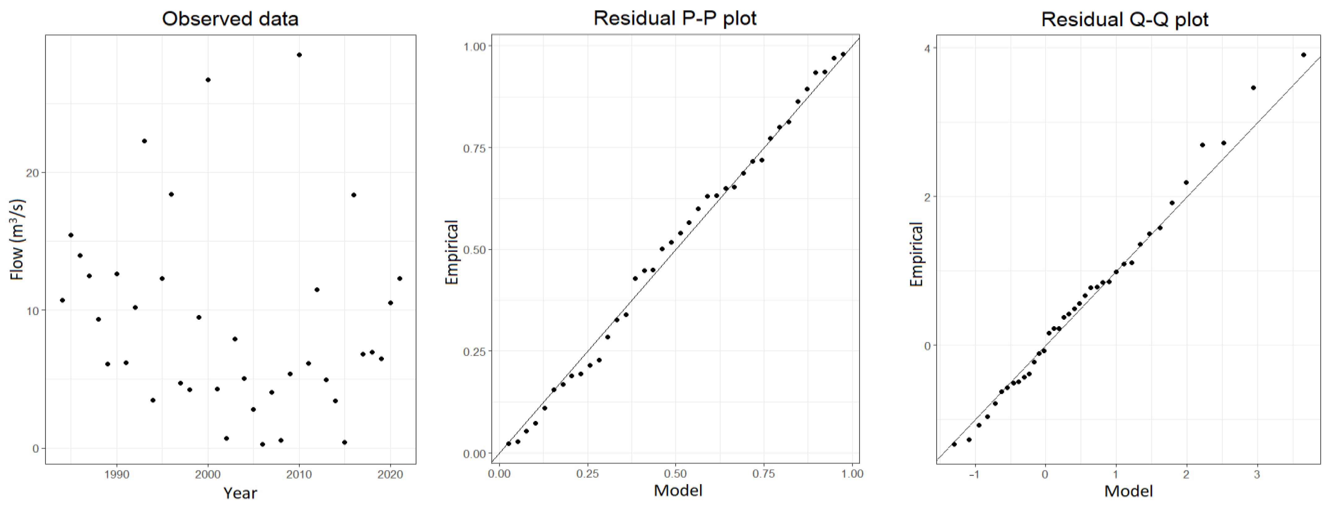
In general, diagnostic plots agree with the statistical tests about goodness of fit of the GEV models. As an example of diagnostic plots, Figure 3 shows the observed AMF data and residual P-P and Q-Q plots of the best fitting model (i.e., NSGEV5) for Station 406250.
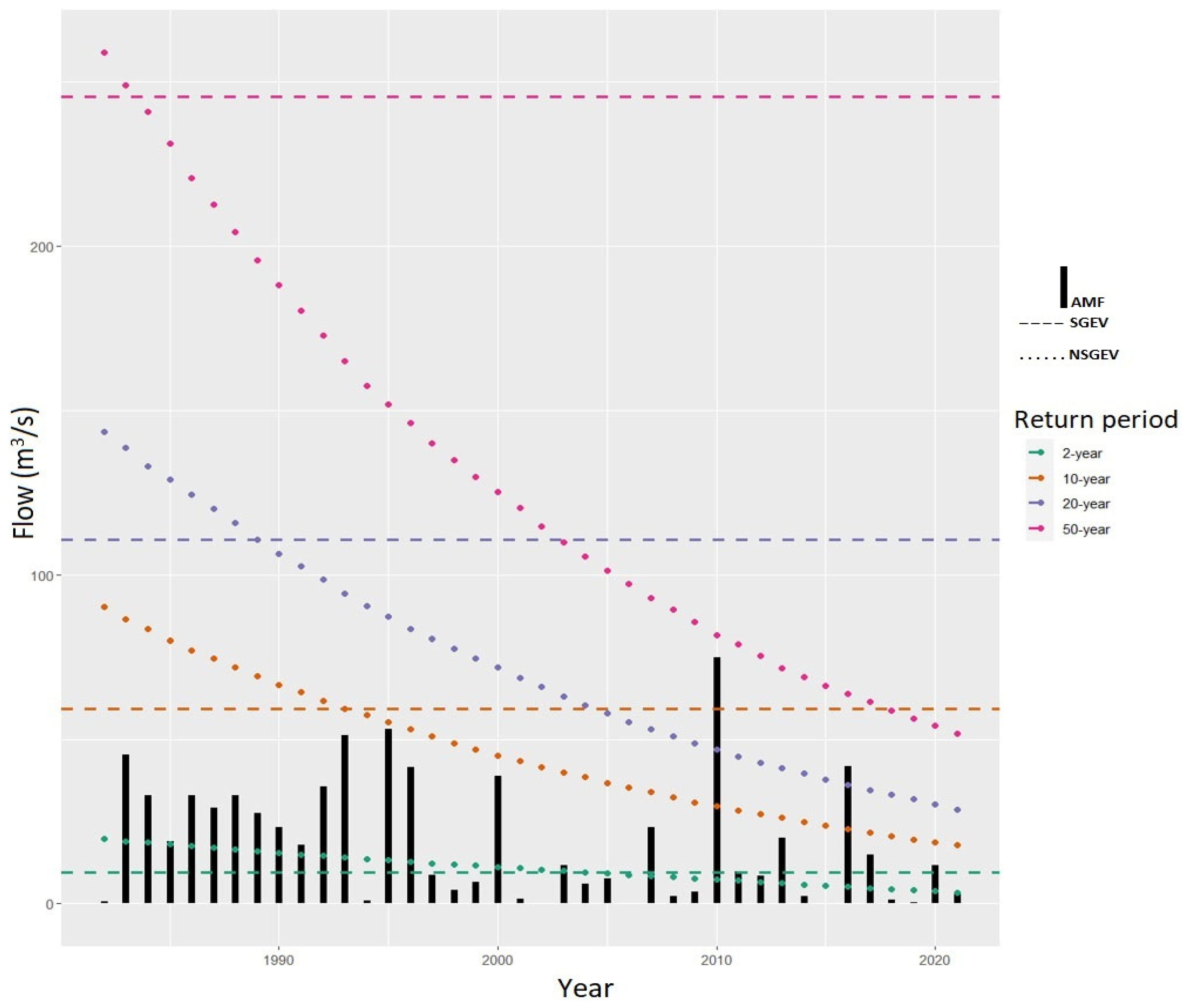
The purpose of a flood frequency analysis is to derive design floods (return levels) for different return periods such as 2, 5, 10, 20, 50, and 100 years. As explained in the Introduction section, a design flood is an essential input for water infrastructure design and water resource management. In this study, design floods were derived for 2-, 10-, 20-, and 50-year return periods along with the 90% confidence intervals for all GEV models at all stations. It is not reasonable to estimate a 100-year design flood with high accuracy, considering the maximum number of data points employed in this study is 53. As an example, Table 6 illustrates the 2-, 10-, 20-, and 50-year design floods for Station 406235 derived from SGEV and NSGEV15 (the best performing GEV model). The same information (design flood estimations from SGEV and NSGEV15 for 2-, 10-, 20-, and 50-year return periods at Station 406235) is shown in Figure 4, where dashed lines indicate design flood estimation of SGEV models and dotted lines show design flood estimation of NSGEV models for abovementioned return periods. As explained in the Methodology section, the uncertainty in GEV models was assessed through 90% confidence intervals, and derived design floods in this study fall into the 90% confidence intervals.
As can be seen in Table 6 and Figure 4, the design flood estimates of NSGEV15 are decreasing over time at Station 406235. In Figure 4, the horizontal lines indicate the design flood estimation from the SGEV model for certain return periods. Design flood estimates of SGEV for 2-, 10-, 20-, and 50-year return periods at Station 406235 are 9.5 m3/s, 59.2 m3/s, 110.7 m3/s, and 245.5 m3/s, respectively. As the parameters of the SGEV model are constant, design flood estimates from the SGEV model do not show variation over time. This is specifically important for Stations 406235 and 406250, where NSGEV outperformed the SGEV counterpart. For example, the difference between 20-year design floods of SGEV and NSGEV models at Station 406235 is −74% in 2021. Table 7 indicates the change percentage of 2-, 10-, 20-, and 50-year design floods in 2021 between SGEV and the best fitting NSGEV for the stations where the NSGEV model showed better fitting than the SGEV (i.e., Stations 406235 and 406250).
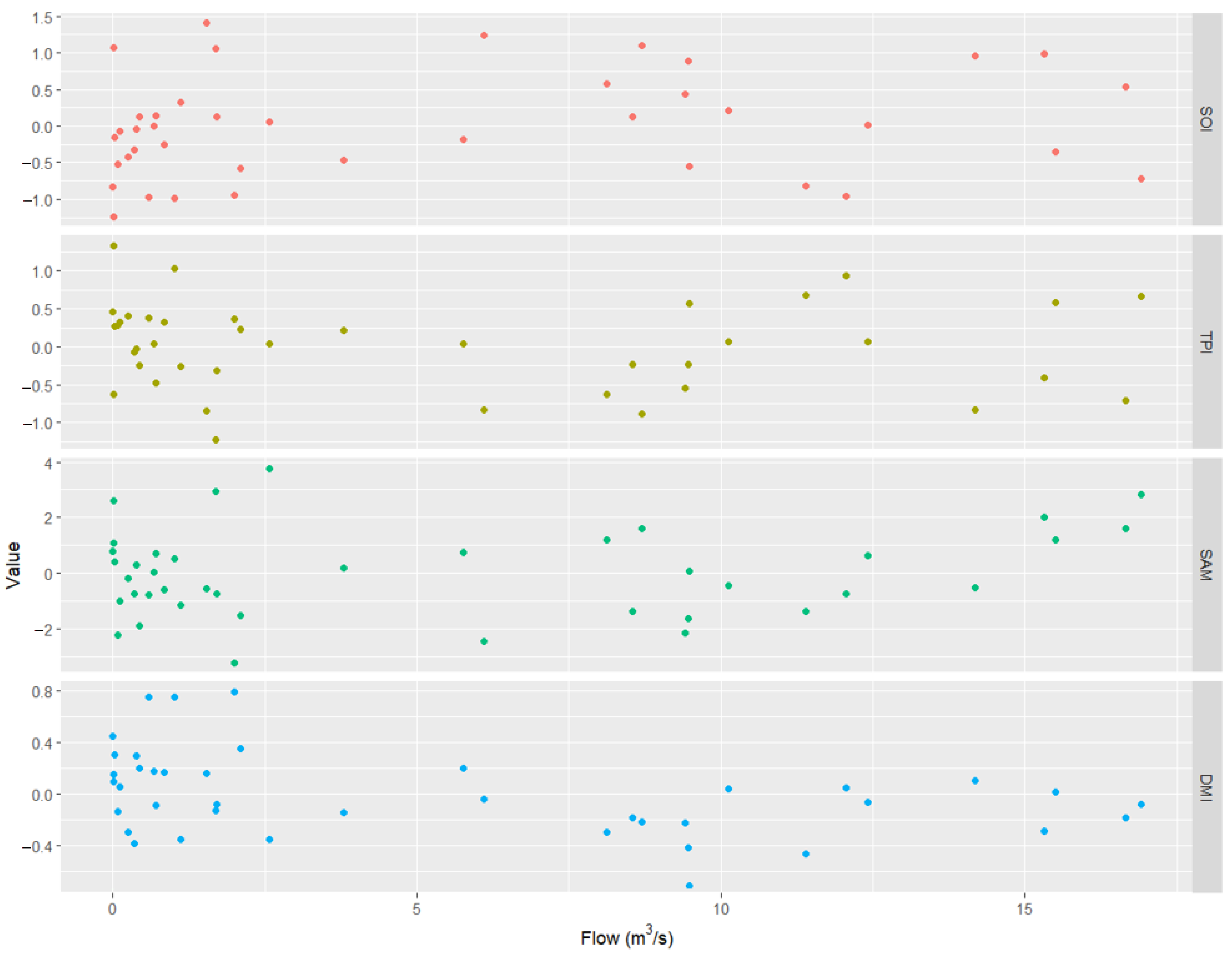
As shown in Table 7, the design floods in 2021 derived from non-stationary models were lower than those derived from stationary models. The difference between non-stationary and stationary models is particularly significant for Station 406235 where the NSGEV15 model was the preferred model. In those stations (in which non-stationary GEV models should be preferred), deriving a design flood from conventional stationary models will result in overestimation of the design flood. This will cause uneconomical water infrastructure design and poor water resource planning and management. As explained in the Methodology section, effects of ENSO, IOD, IPO, and SAM climate drivers on AMFs were investigated in this study through associating SOI, DMI, TPI, and SAM index as a physical covariate to the non-stationary GEV models. It is found that none of the non-stationary GEV models with the physical covariate overperformed the GEV counterpart models. This is the case for all the stations in the study basin. Therefore, there is insufficient evidence to express the AMF non-stationarity in relation to the studied climate drivers. Figure 5 shows the flow data plotted against physical covariates at Station 406208 to examine whether flow is correlated with the covariates used. As can be seen from Figure 5, there is no strong correlation between AMF and physical covariates (SOI, DMI, SAM, and TPI).
The methodology developed in this study can be applied to different study areas by substituting data specific to the region under consideration. This methodology has the potential to yield more accurate design flood estimations, contributing to the successful design and operation of water infrastructure systems. In this study, non-stationary models were developed by considering one covariate at a time for the location and/or scale parameters, following a similar approach adopted by several studies (e.g., [39,48]) in the literature. In the next phase, a multivariate linear and non-linear regression analysis of the covariates in the non-stationary models will be conducted. Furthermore, the performance of different statistical distributions, such as Log-Pearson Type 3 and Generalized Pareto, can be investigated in future studies.

5. Conclusions

In this study, non-stationarity of annual maximum floods (AMFs) was investigated through a methodology consisting of the MK trend test, Pettitt change point test, and non-stationary GEV models, and the methodology was applied to Campaspe River Basin using data from six flow stations located at the outlet of the represented sub-basins. Below are the main conclusions from this study:
  • Statistically significant decreasing trends (at 0.01 and 0.05 significance levels) in AMFs were detected regarding almost all stations in Campaspe River Basin.
  • The year 1996 was identified as the statistically significant change point at almost all stations.
  • Non-stationary GEV models had a time covariate that outperformed the stationary counterparts for two stations (Stations 406235 and 406250).
  • The difference between the design floods of SGEV and NSGEV is particularly important for the NSGEV15 model with time-varying location and scale parameters.
  • There is not enough evidence to state that ENSO, SAM, IOD, or IPO had significant effects on AMF non-stationarity in the basin.
In this study, annual average index values (SOI, DMI, TPI, and SAM index) representing the climate drivers were used. It is worth investigating effects of monthly and/or seasonal index values on the AMF non-stationarity instead of the averaged index in future studies. Also, it is recommended to employ other physical covariates such as annual rainfall, existence of reservoirs (for the disturbed basins), and land use (change) in non-stationary GEV models in future studies.

Author Contributions

Conceptualization, A.G.Y., M.A.I., A.S., R.A.-R. and S.A.; methodology, A.G.Y., S.A. and K.H.; software, A.G.Y.; validation, S.A. and K.H.; original draft preparation, A.G.Y.; writing—review and editing, M.A.I., A.S., R.A.-R. and S.A. All authors have read and agreed to the published version of the manuscript.

Funding

This research received no external funding.

Data Availability Statement

Data can be requested from the corresponding author.

Acknowledgments

Authors would like to thank Bureau of Meteorology, Australia, for providing data.

Conflicts of Interest

There is no conflict of interest.

References

  1. Chen, M.; Papadikis, K.; Jun, C. An investigation on the non-stationarity of flood frequency across the UK. J. Hydrol. 2021, 597, 126309. [Google Scholar] [CrossRef]
  2. Rahman, A.S.; Rahman, A.; Zaman, M.A.; Haddad, K.; Ahsan, A.; Imteaz, M. A study on selection of probability distributions for at-site flood frequency analysis in Australia. Nat. Hazards 2013, 69, 1803–1813. [Google Scholar] [CrossRef]
  3. Yilmaz, A.G.; Pereira, B.J.C. Extreme rainfall non-stationarity investigation and intensity-frequency-duration relationship. ASCE J. Hydrol. Eng. 2014, 19, 1160–1172. [Google Scholar] [CrossRef]
  4. Wasko, C.; Westra, S.; Nathan, R.; Orr, H.G.; Villarini, G.; Herrera, R.V.; Fowler, H.J. Incorporating climate change in flood estimation guidance. Philos. Trans. R. Soc. A Math. Phys. Eng. Sci. 2021, 379, 20190548. [Google Scholar] [CrossRef] [PubMed]
  5. Khaliq, M.N.; Ouarda, T.B.M.J.; Ondo, J.-C.; Gachon, P.; Bobée, B. Frequency analysis of a sequence of dependent and/or non-stationary hydro-meteorological observations: A review. J. Hydrol. 2006, 329, 534–552. [Google Scholar] [CrossRef]
  6. Yilmaz, A.G.; Hossain, I.; Perera, B.J.C. Effect of climate change and variability on extreme rainfall intensity–frequency–duration relationships: A case study of Melbourne. Hydrol. Earth Syst. Sci. 2014, 18, 4065–4076. [Google Scholar] [CrossRef]
  7. Hesarkazzazi, S.; Arabzadeh, R.; Hajibabaei, M.; Rauch, W.; Kjeldsen, T.R.; Prosdocimi, I.; Castellarin, A.; Sitzenfrei, R. Stationary vs. non-stationary modelling of flood frequency distribution across northwest England. Hydrol. Sci. J. 2021, 66, 729–744. [Google Scholar] [CrossRef]
  8. Šraj, M.; Viglione, A.; Parajka, J.; Blöschl, G. The influence of non-stationarity in extreme hydrological events on flood frequency estimation. J. Hydrol. Hydromech. 2016, 64, 426–437. [Google Scholar] [CrossRef]
  9. Ray, L.K.; Goel, N.K. Flood Frequency Analysis of Narmada River Basin in India under Nonstationary Condition. J. Hydrol. Eng. 2019, 24, 05019018. [Google Scholar] [CrossRef]
  10. Singh, N.; Chinnasamy, P. Non-stationary flood frequency analysis and attribution of streamflow series: A case study of Periyar River, India. Hydrol. Sci. J. 2021, 66, 1866–1881. [Google Scholar] [CrossRef]
  11. Hounkpè, J.; Diekkrüger, B.; Badou, D.F.; Afouda, A.A. Non-Stationary Flood Frequency Analysis in the Ouémé River Basin, Benin Republic. Hydrology 2015, 2, 210–229. [Google Scholar] [CrossRef]
  12. Bossa, A.Y.; Akpaca, J.d.D.; Hounkpè, J.; Yira, Y.; Badou, D.F. Non-Stationary Flood Discharge Frequency Analysis in West Africa. GeoHazards 2023, 4, 316–327. [Google Scholar] [CrossRef]
  13. Anzolin, G.; Chaffe, P.L.B.; Vrugt, J.A.; AghaKouchak, A. Using climate information as covariates to improve nonstationary flood frequency analysis in Brazil. Hydrol. Sci. J. 2023, 68, 645–654. [Google Scholar] [CrossRef]
  14. Ishak, E.H.; Rahman, A.; Westra, S.; Sharma, A.; Kuczera, G. Evaluating the non-stationarity of Australian annual maximum flood. J. Hydrol. 2013, 494, 134–145. [Google Scholar] [CrossRef]
  15. Do, H.X.; Zhao, F.; Westra, S.; Leonard, M.; Gudmundsson, L.; Boulange, J.E.S.; Müller Schmied, H. Historical and future changes in global flood magnitude–evidence from a model-observation investigation. Hydrol. Earth Syst. Sci. 2020, 24, 1543–1564. [Google Scholar] [CrossRef]
  16. Ishak, E.; Rahman, A. Examination of Changes in Flood Data in Australia. Water 2019, 11, 1734. [Google Scholar] [CrossRef]
  17. Yilmaz, A.G. Climate change effects and extreme rainfall non-stationarity. ICE-Water Manag. 2017, 170, 57–65. [Google Scholar] [CrossRef]
  18. Han, X.; Mehrotra, R.; Sharma, A.; Rahman, A. Incorporating nonstationarity in regional flood frequency analysis procedures to account for climate change impact. J. Hydrol. 2022, 612, 128235. [Google Scholar] [CrossRef]
  19. Faulkner, D.; Warren, S.; Spencer, P.; Sharkey, P. Can we still predict the future from the past? Implementing non-stationary flood frequency analysis in the UK. J. Flood Risk Manag. 2020, 13, e12582. [Google Scholar] [CrossRef]
  20. Zhang, T.; Wang, Y.; Wang, B.; Tan, S.; Feng, P. Nonstationary Flood Frequency Analysis Using Univariate and Bivariate Time-Varying Models Based on GAMLSS. Water 2018, 10, 819. [Google Scholar] [CrossRef]
  21. Goulburn-Murray Water (GMW). 2022. Available online: https://www.g-mwater.com.au/water-operations/catchments/campaspebasin (accessed on 15 December 2022).
  22. Murray-Darling Basin Authority (MDBA). 2022. Available online: https://www.mdba.gov.au/water-management/catchments/campaspe (accessed on 10 December 2022).
  23. Bureau of Meteorology (BoM). 2022. Available online: http://www.bom.gov.au/water/hrs/ (accessed on 5 October 2022).
  24. Yue, S.; Pilon, P.; Cavadias, G. Power of the Mann–Kendall and Spearman’s rho tests for detecting monotonic trends in hydrological series. J. Hydrol. 2002, 259, 254–271. [Google Scholar] [CrossRef]
  25. Laz, O.U.; Rahman, A.; Yilmaz, A.; Haddad, K. Trends in sub hourly, sub daily and daily extreme rainfall events in eastern Australia. J. Water Clim. Chang. 2014, 5, 667–675. [Google Scholar] [CrossRef]
  26. Wagesho, N.; Goel, N.K.; Jain, M.K. Investigation of non-stationarity in hydro-climatic variables at Rift Valley lakes basin of Ethiopia. J. Hydrol. 2012, 444–445, 113–133. [Google Scholar] [CrossRef]
  27. Yilmaz, A.G. The effects of climate change on historical and future extreme rainfall in Antalya, Turkey. Hydrol. Sci. J. 2015, 60, 2148–2162. [Google Scholar] [CrossRef]
  28. Yilmaz, A.G.; Perera, B.J.C. Spatiotemporal Trend Analysis of Extreme Rainfall Events in Victoria, Australia. Water Resour. Manag. 2015, 29, 4465–4480. [Google Scholar] [CrossRef]
  29. Kundzewicz, Z.W.; Robson, A. Detecting Trend and Other Changes in Hydrological Data; WCDMP, No. 45; WMO-TD, No. 1013; WMO: Geneva, Switzerland, 2000. [Google Scholar]
  30. Diop, L.; Yaseen, Z.M.; Bodian, A.; Djaman, K.; Brown, L. Trend analysis of streamflow with different time scales: A case study of the upper Senegal River. ISH J. Hydraul. Eng. 2018, 24, 105–114. [Google Scholar] [CrossRef]
  31. Guclu, Y.S. Improved visualization for trend analysis by comparing with classical MannKendall test and ITA. J. Hydrol. 2020, 584, 124674. [Google Scholar] [CrossRef]
  32. Conte, L.C.; Débora, M.B.; Fábio, M.B. Bootstrap Pettitt test for detecting change points in hydroclimatological data: Case study of Itaipu Hydroelectric Plant, Brazil. Hydrolog. Sci. J. 2019, 64, 1312–1326. [Google Scholar] [CrossRef]
  33. Engeland, K.; Aano, A.; Steffensen, I.; Støren, E.; Paasche, Ø. New flood frequency estimates for the largest river in Norway based on the combination of short and long time series. Hydrol. Earth Syst. Sci. 2020, 24, 5595–5619. [Google Scholar] [CrossRef]
  34. Park, J.-S.; Kang, H.-S.; Lee, Y.S.; Kim, M.-K. Changes in the extreme daily rainfall in South Korea. Int. J. Clim. 2010, 31, 2290–2299. [Google Scholar] [CrossRef]
  35. Haddad, K.; Rahman, A. Selection of the best fit flood frequency distribution and parameter estimation procedure: A case study for tasmania in australia. Stoch. Environ. Res. Risk Assess. 2011, 25, 415–428. [Google Scholar] [CrossRef]
  36. Liu, J.; Zhang, Y.; Yang, Y.; Gu, X.; Xiao, M. Investigating Relationships Between Australian Flooding and Large-Scale Climate Indices and Possible Mechanism. J. Geophys. Res. Atmos. 2018, 123, 8708–8723. [Google Scholar] [CrossRef]
  37. Johnson, F.; White, C.J.; van Dijk, A.; Ekstrom, M.; Evans, J.P.; Jakob, D.; Kiem, A.S.; Leonard, M.; Rouillard, A.; Westra, S. Natural Hazards in Australia: Floods. Clim. Chang. 2016, 139, 21–35. [Google Scholar] [CrossRef]
  38. Tramblay, Y.; Neppel, L.; Carreau, J.; Najib, K. Non-stationary frequency analysis of heavy rainfall events in southern France. Hydrol. Sci. J. 2013, 58, 280–294. [Google Scholar] [CrossRef]
  39. De Paola, F.; Giugni, M.; Pugliese, F.; Annis, A.; Nardi, F. GEV parameter estimation and stationary vs. non-stationary analysis of extreme rainfall in African test cities. Hydrology 2018, 5, 28. [Google Scholar] [CrossRef]
  40. Xavier, A.C.F.; Rudke, A.P.; Fujita, T.; Blain, G.C.; De Morais, M.V.B.; De Almeida, D.S.; Rafee, S.A.A.; Martins, L.D.; De Souza, R.A.F.; De Freitas, E.D.; et al. Stationary and Non-Stationary Detection of Extreme Precipitation Events and Trends of Average Precipitation from 1980 to 2010 in the Paraná River Basin, Brazil. Int. J. Climatol. 2020, 40, 1197–1212. [Google Scholar] [CrossRef]
  41. UK Environment Agency. Development of Interim National Guidance on Non-Stationary Fluvial Flood Frequency Estimation –R Package Nonstat User Guide. 2020. Available online: https://assets.publishing.service.gov.uk/media/6038f77de90e070555cedc22/non-stationary_fluvial_flood_frequency_estimation_-_package_user_guide.pdf (accessed on 3 March 2023).
  42. Dodangeh, E.; Singh, V.P.; Pham, B.T.; Yin, J.; Yang, G.; Mosavi, A. Flood frequency analysis of interconnected Rivers by copulas. Water Resour. Manag. 2020, 34, 3533–3549. [Google Scholar] [CrossRef]
  43. Echogdali, F.Z.; Rosine, B.K.; Ouchchen, M.; Id-Belqas, M.; Dadi, B.; Ikirri, M.; Abioui, M.; Boutaleb, S. Spatial Prediction of Flood Frequency Analysis in a Semi-Arid Zone: A Case Study from the Seyad Basin (Guelmim Region, Morocco). In Geospatial Technology for Landscape and Environmental Management; Rai, P.K., Mishra, V.N., Singh, P., Eds.; Springer: Singapore, 2022. [Google Scholar] [CrossRef]
  44. Coles, S. An Introduction to Statistical Modeling of Extreme Values; Springer-Verlag Inc.: London, UK, 2001. [Google Scholar]
  45. Eastoe, E.M.; Tawn, J.A. Modelling non-stationary extremes with application to surface level ozone. J. R. Stat. Soc. Ser. C Appl. Stat. 2009, 58, 25–45. [Google Scholar] [CrossRef]
  46. Lu, H.; Bryant, R.B.; Buda, A.R.; Collick, A.S.; Folmar, G.J.; Kleinman, P.J.A. Long-term trends in climate and hydrology in an agricultural, headwater watershed of central Pennsylvania, USA. J. Hydrol. Reg. Stud. 2015, 4, 713–731. [Google Scholar] [CrossRef]
  47. Basarin, B.; Lukić, T.; Pavić, D.; Wilby, R.L. Trends and multi-annual variability of water temperatures in the river Danube, Serbia. Hydrol. Process. 2016, 30, 3315–3329. [Google Scholar] [CrossRef]
  48. Razmi, A.; Golian, S.; Zahmatkesh, Z. Non-Stationary Frequency Analysis of Extreme Water Level: Application of Annual Maximum Series and Peak-over Threshold Approaches. Water Resour. Manag. 2017, 31, 2065–2083. [Google Scholar] [CrossRef]
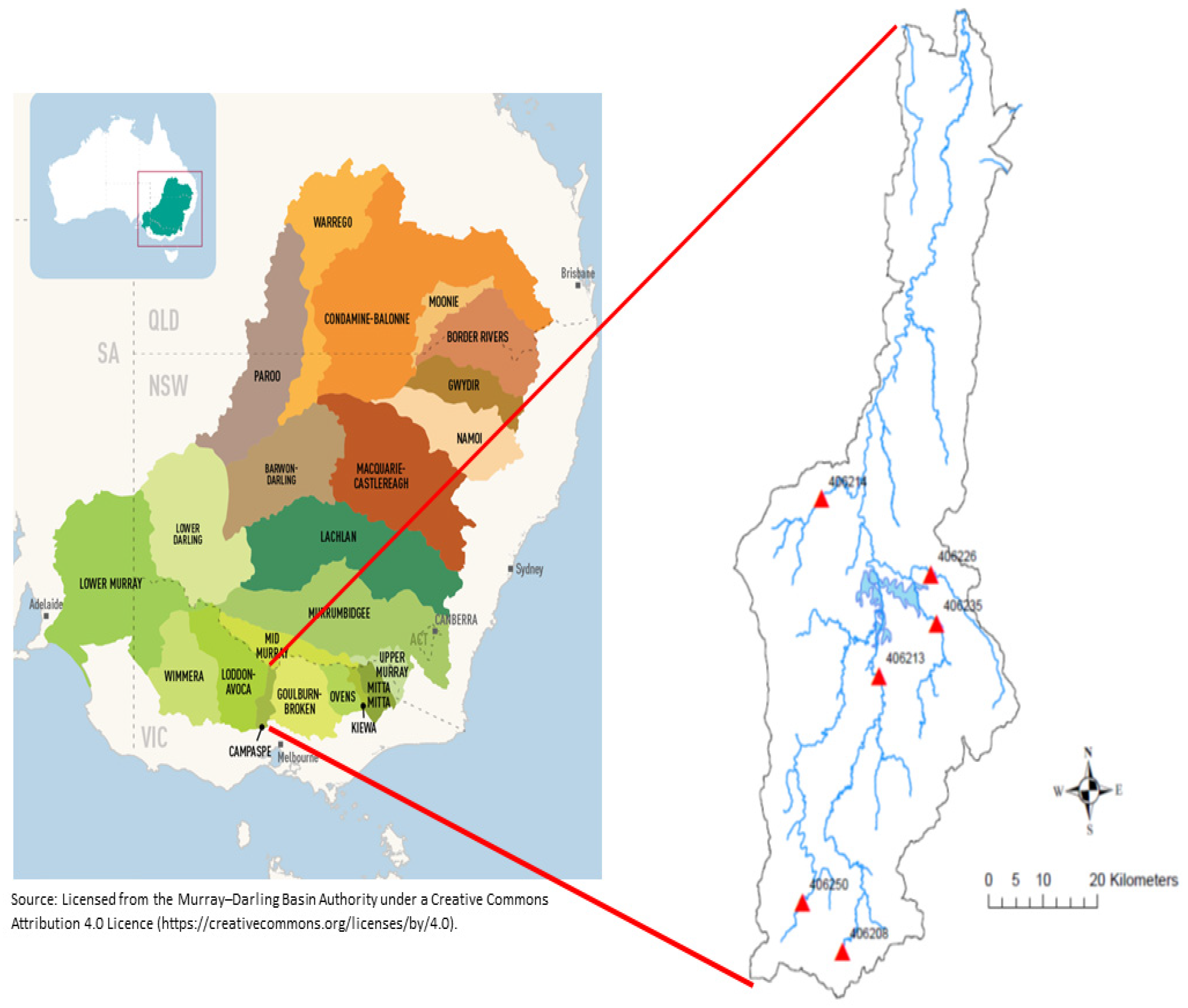
Figure 1. Location of the Campaspe River Basin and selected stations.
Water 15 03683 g001
Figure 2. Trend and autocorrelation graphs for AMF at Stations 406208 and 406214.
Water 15 03683 g002
Figure 3. Observed data and residual P-P and Q-Q plots of NSGEV5 for Station 406250.
Water 15 03683 g003
Figure 4. Design flood estimations from SGEV and NSGEV15 for 2-, 10-, 20-, and 50-year return periods at Station 406235.
Water 15 03683 g004
Figure 5. Correlation between AMF and physical covariates (SOI, TPI, SAM, and DMI).
Water 15 03683 g005
Table 1. Location, sub-basin area, and available data period of selected stations.
Station NumberSub-Basin Area (km2)LocationAvailable Data Period
40620837.6144.451° E, 37.388° S1970–2022
406213633.8144.539° E, 37.016° S1975–2022
406214237144.428° E, 36.774° S1972–2022
406226171.6144.650° E, 36.881° S1978–2022
406235212.3144.660° E, 36.948° S1980–2022
40625077.5144.370° E, 37.320° S1983–2022
Table 2. Developed non-stationary GEV models.
Model NameParameters of Model
μ l n σ   =   ϕ ξ
NSGEV1 μ ( x ) = μ 0 + μ 1 × S O I Constant Constant
NSGEV2 μ ( x ) = μ 0 + μ 1 × T P I Constant Constant
NSGEV3 μ ( x ) = μ 0 + μ 1 × S A M Constant Constant
NSGEV4 μ ( x ) = μ 0 + μ 1 × D M I Constant Constant
NSGEV5 μ ( t ) = μ 0 + μ 1 × t Constant Constant
NSGEV6Constant ϕ x = ϕ 0 + ϕ 1 × S O I Constant
NSGEV7Constant ϕ ( x ) = ϕ 0 + ϕ 1 × T P I Constant
NSGEV8Constant ϕ ( x ) = ϕ 0 + ϕ 1 × S A M Constant
NSGEV9Constant ϕ ( x ) = ϕ 0 + ϕ 1 × D M I Constant
NSGEV10Constant ϕ ( t ) = ϕ 0 + ϕ 1 × t Constant
NSGEV11 μ ( x ) = μ 0 + μ 1 × S O I ϕ x = ϕ 0 + ϕ 1 × S O I Constant
NSGEV12 μ ( x ) = μ 0 + μ 1 × T P I ϕ ( x ) = ϕ 0 + ϕ 1 × T P I Constant
NSGEV13 μ ( x ) = μ 0 + μ 1 × S A M ϕ ( x ) = ϕ 0 + ϕ 1 × S A M Constant
NSGEV14 μ ( x ) = μ 0 + μ 1 × D M I ϕ ( x ) = ϕ 0 + ϕ 1 × D M I Constant
NSGEV15 μ ( t ) = μ 0 + μ 1 × t ϕ ( t ) = ϕ 0 + ϕ 1 × t Constant
Table 3. Trend analysis results.
Station Numberz-Score2-Sided p-ValueOutcome
406208−3.661570.000250671S (0.01)
406213−2.367040.017931094S (0.05)
406214−3.663430.00024886S (0.01)
406226−2.606030.009159779S (0.01)
406235−2.594580.00947072S (0.01)
406250−1.458340.144746587NS
Table 4. Change point analysis (Pettitt test) results.
Station Numberp-ValueOutcomeYear of Change
4062080.000295S (0.01)1996
4062130.010492S (0.05)1996
4062140.002299S (0.01)1996
4062260.015921S (0.05)1996
4062350.016234S (0.05)1996
4062500.088723NS2000
Table 5. Stationary and non-stationary model parameters and performances.
Gauge NumberModel Location μ 0 Location μ 1 Ln   ( Scale )   ϕ 0 Ln   ( Scale )   ϕ 1 ShapeAICBIC
406208SGEV0.9068 0.4415 1.4555226231
406208NSGEV50.88030.02260.4322 1.4738228235
406208NSGEV151.4105−0.66660.7438−0.65791.0779225233
406213SGEV12.9959 2.8779 1.0512406411
406213NSGEV512.61470.53002.8679 1.0701408415
406213NSGEV1515.3868−4.13443.0092−0.45800.8058406414
406214SGEV1.4513 1.1221 2.026300305
406214NSGEV51.28990.04991.0587 2.1561301308
406214NSGEV152.3495−0.92211.4599−0.66611.3696301309
406226SGEV2.1333 1.2295 1.2554282287
406226NSGEV52.1347−0.00041.2300 1.2552284290
406226NSGEV152.9686−1.28841.3622−0.54550.8445280288
406235SGEV6.1003 2.0935 0.8171334339
406235NSGEV56.5611−0.42832.1262 0.7407335342
406235NSGEV157.7278−3.44822.1293−0.47840.5273330338
406250SGEV5.8260 1.5449 0.1154249253
406250NSGEV55.8056−1.96011.4617 0.1721247253
406250NSGEV155.7582−2.15431.45270.13180.1695248256
Table 6. Design floods for 2-, 10-, 20-, and 50-year return periods at Station 406235.
YearNSGEV15
(2-Year)
NSGEV15
(10-Year)
NSGEV15
(20-Year)
NSGEV15
(50-Year)
198219.790.2143.4258.8
198319.186.5138.6249.0
198418.683.5133.0241.0
198518.180.1128.9231.1
198617.677.2124.5220.8
198717.174.6120.1212.6
198816.572.0115.7204.2
198916.069.3110.6195.7
199015.566.5106.5188.2
199115.064.3102.5180.4
199214.561.898.5172.7
199314.159.494.2165.0
199413.657.390.6157.6
199513.255.287.2151.8
199612.853.283.4146.2
199712.451.080.6139.9
199812.048.977.5134.8
199911.646.974.6129.7
200011.245.172.0125.3
200110.843.368.6120.5
200210.441.766.0114.8
200310.039.963.2110.0
20049.738.560.5105.6
20059.336.858.1101.4
20068.935.455.497.4
20078.533.953.193.0
20088.132.451.089.5
20097.730.948.785.7
20107.429.646.881.8
20117.028.444.878.9
20126.627.343.075.3
20136.326.141.271.7
20145.924.939.669.0
20155.523.837.866.3
20165.222.836.163.8
20174.821.734.661.4
20184.420.533.358.7
20194.119.631.956.3
20203.818.630.354.2
20213.417.828.751.8
Table 7. The change percentage of 2-, 10-, 20-, and 50-year design floods in 2021.
Station 406235Station 406250
StationaryNon-StationaryChange (%)StationaryNon-StationaryChange (%)
2-year
Design Flood (m3/s)
9.53.4−647.64.1−46
10-year
Design Flood (m3/s)
59.217.8−7017.613.9−21
20-year
Design Flood (m3/s)
110.728.7−7421.918.6−15
50-year
Design Flood (m3/s)
245.551.8−7928.125.8−8
Disclaimer/Publisher’s Note: The statements, opinions and data contained in all publications are solely those of the individual author(s) and contributor(s) and not of MDPI and/or the editor(s). MDPI and/or the editor(s) disclaim responsibility for any injury to people or property resulting from any ideas, methods, instructions or products referred to in the content.