Research on the Standardized Management System and Operational Indicators of Water Control Dikes Based on GA-BP Artificial Neural Network Model

Abstract

Water control dikes, as an important infrastructure for national economic and social development, play an important supporting and guaranteeing role in flood control, irrigation, power generation, water supply, tourism, and other aspects. Jiangxi is a major province in water conservancy, with dense rivers and lakes, and it owns tens of thousands of water control dikes of various types. Most of the water control dikes exhibit structural aging, continuous medical risks, and reduced benefits, which urgently require efficient maintenance and standardized management. Management is a complex task, and the level of management directly affects the functional efficiency and service life of dikes. In view of these issues, this study takes dikes as essential and typical water conservancy engineering objects and analyzes the evaluation criteria of safe production and the demands of engineering management. It establishes an evaluation index system suitable for normalized management. The Analytic Hierarchy Process (AHP) model is utilized to determine indicator weights, and a neural network water conservancy engineering evaluation algorithm is constructed to match the evaluation model. Finally, an improved algorithm for the GA (genetic algorithm)-BP (backpropagation) neural network is proposed, incorporating additional momentum factors and considering adaptive learning rates. The developed model is validated through a case study in Jiangxi, China, and the results demonstrate its accuracy and comprehensiveness in reflecting the actual situation. This research is relevant to designers, contractors, and governments seeking solutions to achieve standardized management in water control dikes.

1. Introduction

The “14th Five-Year Plan” of China proposes the need to strengthen water conservancy infrastructure construction to promote the modernization of China’s infrastructure. Dikes, as an important part of water conservancy infrastructure, play a crucial role in ensuring and improving people’s livelihoods and promoting social and economic development. However, dike construction involves land occupation [1], consumption of natural resources (water, raw materials, etc.), energy consumption [2], greenhouse gas emissions [3], and the generation of construction waste [4]. The rapid expansion in scale and quantity of dike construction inevitably leads to environmental issues. Therefore, it is urgent to achieve sustainable development of water conservancy projects and evaluate the safe production of dike construction.

Jiangxi Province is a major province in water conservancy, with hundreds of thousands of various types of dikes playing an important role in flood control, irrigation, power generation, and water supply, making outstanding contributions to regional economic development. Most of these dike projects were constructed in the 1950s to 1970s when the technological level was relatively backward, and there was a lack of strict supervision and management. After the “98” flood, large-scale reinforcement works were carried out by national and local governments, and many projects were able to eliminate safety hazards. However, issues related to operation and management remain prominent, primarily in four aspects: inadequate implementation of management responsibilities, severe shortage of management funds, extensive management practices, and low qualifications of management personnel.

In the context of the national policy of “standardization system construction” and the new era’s general tone of water conservancy development focusing on addressing shortcomings and strengthening regulatory measures, water conservancy standardization has become a key driver for promoting high-quality development in the water conservancy industry. The Water Resources Department of Jiangxi Province promptly issued the “Notice on the Comprehensive Implementation of Standardized Management of Water Conservancy Projects” and various assessment scoring standards for standardized management. In 2019 and 2020, the evaluation indicators were integrated and summarized, resulting in more than 20 evaluation criteria in four categories: safety management, operation management, maintenance management, and management support. After three years of comprehensive implementation, over 13,000 water conservancy projects in the province have passed the evaluation and met the standards. Starting in 2021, the standardized management of water conservancy projects has entered the stage of consolidation and improvement, with a focus on promoting the normalization of standardized management for projects that have already met the standards.

Currently, research on safe production in water conservancy projects mainly focuses on three aspects: (1) The development process of green construction and safe production: In the 1960s, Paola Soleri first emphasized the relationship between construction and the environment as a key research topic. In the 1980s, the concept of sustainable development was formally proposed at environmental conferences [5]. Subsequently, Charles Kibert defined the concept of sustainable construction, emphasizing the efficient use of resources, minimizing environmental pollution, and its impact on human health during the construction process [6]. In the 1990s, research on green construction started in China, while internationally, green construction standards were already being established, such as BREEAM by the Building Research Establishment Ltd. in the UK and LEED by the US Green Building Council [7,8]. During this period, Professor Laure Koslda (1992) introduced the concept of “lean construction”, which aims to reduce environmental damage and minimize the waste of water, electricity, materials, and oil by improving construction management practices [9]. In the early 21st century, green construction gained increasing attention. Isabelina Nahmens (2009) argued that the transition from lean construction to green construction signifies a shift in construction project management from solely pursuing economic maximization to considering environmental impacts, social contributions, and long-term project benefits [10]. Chrisna (2007) suggested that developing countries should avoid the approach of “pollute first, then treat” when promoting infrastructure development [11]. Mohd (2012) and others proposed the promotion of green construction concepts to facilitate sustainable development in construction projects in Malaysia [12]. Circo (2008) advocated for more land-use policies by the US government to promote the development of green buildings [13]. L.B. Robichaud (2010) suggested optimizing cost structures to reduce cost control factors that restrict the development of green construction in the building industry [14]. Other international scholars have concluded from literature research that companies need to balance various factors, such as cost and productivity, in the context of green construction. (2) Research on safe production evaluation: In terms of green construction evaluation, the Building Research Establishment Ltd. in the UK summarized the evaluation categories as energy use, ecological environment, transportation facilities, environmental protection, site utilization, construction materials, water environment, and public health, with rating levels of excellent, good, fair, and pass. The US Green Building Council’s evaluation of green buildings includes site design, indoor environmental quality, technological innovation, and the utilization of resources, energy, materials, and water, with rating levels of platinum, gold, silver, and certified. Regarding evaluation methods for safe production, a considerable number of scholars used the Analytic Hierarchy Process (AHP) for evaluation in the early stage [15,16]. (3) Research on intelligent information processing and machine learning in safe production management: Scholars such as Wang Shou-Jue (2002) from the Institute of Semiconductors, Chinese Academy of Sciences, conducted application research in the field of pattern recognition [17]. Zhou Zhihua (2003) and others from Nanjing University proposed the GAFNE neural network model for medical diagnosis [18]. Liao Xiaofeng (2001; 2002) and others from Southwest University researched the stability and robustness of neural networks, which have been widely applied in pattern recognition and automatic control [19,20,21]. Scholars such as Ni Shenhai (2000) applied artificial neural network theory and methods to establish a BP artificial neural network model for groundwater quality evaluation, significantly improving the accuracy of groundwater quality evaluation for the Six Eye Wells in Hefei City [22]. Zhu Qihong (2003) proposed an evaluation model for enterprise knowledge management based on artificial neural networks, which proved to be feasible and effective in enterprise knowledge management evaluation [23]. Wang Meiling (2009) proposed an improved BP artificial neural network algorithm, which adjusts the classical neuron transfer function by introducing new parameters [24]. The algorithm was applied to actual teaching evaluations, and appropriate parameter values were selected based on the analysis results of real data. Yan Bin (2008) proposed the application of radial basis function neural networks in the comprehensive safety evaluation of dikes, which was applied to dike safety evaluations [25]. Wang Aihua and Sun Jun (2009) proposed a BP artificial neural network-based model flowchart for engineering project management and provided corresponding suggestions for the parameter settings of the BP artificial neural network application [26,27].

With the rapid development of artificial intelligence, dike management is increasingly integrated with machine learning. The machine-learning-based method, which considers the nonlinear variation of variables, focuses on the selection of input variables and the optimization of model effects. The method has shown great potential in many fields of science and engineering involving data-based prediction. Some researchers developed a support vector regression identification for predicting the behavior of dike structures [28]. Yan et al. (2022) integrated the Faster Region-Convolutional Neural Network (Faster R-CNN) technique with Optical gas imaging (OGI) for automated hydrocarbon leak detection [29]. Li et al. (2022) selected 27 influencing parameters to build a hydraulic structure safety monitoring model based on a Random Forest (RF) intelligent algorithm to predict dam uplift pressure [30]. Dong et al. (2020) constructed an environmental quantity response model using an RBF neural network for anomalous data and established a coupling relationship for tailings dam safety evaluation [31]. Jia et al. (2019) used the GBRT algorithm based on slope monitoring data to improve risk prevention and control [32]. Some scholars have also introduced machine-learning methods to the tailings dam risk prediction problem and achieved good results [33]. The interpretability of the model is poor because machine-learning-based methods cannot extract the significance of each influencing variable. Furthermore, ML-based models are based on time-domain prediction.

Shortcomings of existing evaluation indicators and methods:

The correlation between indicators affects the accuracy of evaluation results to some extent. Traditional evaluation methods, such as the coefficient method, assume that the evaluation indicators are independent of each other. However, if there is a high correlation between evaluation indicators, it can severely affect the accuracy of the evaluation results. In reality, the selected indicators in the current indicator system are not completely independent of each other, and some indicators have a strong correlation. This inherent correlation in the chosen method already implies inaccuracies in the results.

Adjustment is not made for indicators of different natures. In current performance evaluation practices in China, a weighted comprehensive evaluation is commonly used, which requires the weights to be positive. This means that when using these indicators for a comprehensive evaluation, all indicators must reflect the evaluation results in the same direction. Taking the weighted average of indicators with different natures will inevitably lead to a lack of scientific validity in the calculation results. Therefore, it is necessary to separate appropriate indicators from other indicators.

Inability to accurately reflect the diversity of engineering management practices. First, existing evaluation criteria consist of predominantly static indicators such as organizational personnel, funding, systems, and manuals, which carry a higher weightage in scoring. On the other hand, dynamic indicators such as inspections, observations, maintenance, flood control, information management, and record-keeping have relatively less importance. As a result, the evaluation results fail to fully reflect the actual achievements of engineering management units and personnel in their practical management activities. Second, the current evaluation methods primarily rely on traditional expert scoring and brainstorming sessions. The evaluation is mainly based on the records provided by the management units and the prepared acceptance materials, which do not fully capture the daily management activities of the personnel. Consequently, the subjectivity and arbitrariness of the experts during the scoring process are high, therefore impacting the accuracy and objectivity of the evaluation indicators.

However, the existing evaluation criteria are more suitable for short-term assessment of standardized management creation and are not suitable for assessing long-term dynamic standardized management processes. Therefore, this study focuses on key dike projects in the province and aims to establish a comprehensive evaluation system with reasonable assessment indicators from the perspectives of safety, operation, and maintenance. Adopting advanced evaluation methods and techniques can truly reflect the requirements of safe production in water conservancy projects. The main objectives of this study are:

To improve the management level of management units: By conducting evaluations, establishing a practical evaluation indicator system, and providing evaluation standards, it can help management units conduct in-depth, comprehensive, and thorough analysis, self-assess their current engineering management capabilities, identify strengths, weaknesses, and urgent problems that need to be addressed. This will enable management units to formulate improvement measures and pathways to enhance their engineering management capabilities.

To achieve management goals: Effective management in water conservancy projects involves multiple departments and personnel. Through management capacity evaluations, it is beneficial to assess and supervise the implementation departments and members’ work, achieve management control during the implementation process, and ultimately achieve management assessment goals.

To enhance the competitiveness of units: Evaluations can identify the engineering management capabilities that units possess and areas that need improvement. By implementing improvement measures, units can further enhance their engineering management capabilities.

The research on the establishment of standardized management indicators and evaluation methods is crucial to prevent engineering management units from focusing solely on achieving compliance without neglecting actual management practices. It aims to foster a concept of scientific management and standardized operations among management units and personnel, which is significant in addressing the issue of “heavy construction and light management”. It is necessary to genuinely address the standardization of management.

To address these research gaps, this study aims to establish an indicator-based evaluation model for safe production in dikes, using the Analytic Hierarchy Process (AHP) and GA-BP neural network. The model will systematically and comprehensively assess the impact of standardized management in water conservancy projects on the environment. The remaining sections of this paper are organized as follows: Section 2 develops the AHP-GA-BP network model for evaluating safe production in dikes. Section 3 demonstrates the developed model through a case study. Section 4 discusses the key factors and improvements of the case project, as well as the generalization and limitations of the model. This section also provides suggestions for future research. Finally, the conclusions are drawn in Section 5.

2. Materials and Methods

The study area is Jiangxi Province. Jiangxi Province is a major province in water conservancy, with hundreds of thousands of various water conservancy projects. It has played an important role in flood control, irrigation, power generation, and water supply and has made outstanding contributions to the development of the regional economy. Most of these water conservancy projects were built in the 1950s to 1970s when the technical level was relatively backward, and the supervision and management were not strict. After the completion of the projects, there were varying degrees of hidden dangers. The study area is shown in Figure 1.

2.1. Standardized Management Indicator System

The evaluation indicators of the standardized management system for dike engineering should comprehensively reflect the various aspects and factors involved in the management content. Based on the basic characteristics, technical means, and key issues of local engineering, combined with expert experience and suggestions, an evaluation index system was constructed. It mainly includes 18 evaluation indicators from 5 categories. The evaluation index system is shown in

Table 1. Evaluation Index System of Standardized Management of Dike Project.

Level 1 Indicator (B)	Secondary Indicator (C)
Management Foundation (B1)	Management Manual (C1)
	Engineering delimitation (C2)
	Management Facilities (C3)
	Archive Management (C4)
Safety Management (B2)	Responsible person (C5)
	Safety Production (C6)
	Emergency Management (C7)
	Flood prevention and control (C8)
Operation Management (B3)	Engineering Inspection (C9)
	Engineering Observation (C10)
	Operation (C11)
Maintenance Management (B4)	Repair and maintenance (C12)
	Equipment maintenance (C13)
	Engineering Image (C14)
Management Assurance (B5)	Position personnel (C15)
	Informatization level (C16)
	Evaluation incentive (C17)
	Management and protection funds (C18)

.

2.1.1. Management Foundation (B1)

In the B1 of Level 1 Indicator, the meanings of Management Manual (C1), Engineering delimitation (C2), Management Facilities (C3), and Archive Management (C4) are shown in

Table 2. Content of management foundation indicators.

Secondary Indicator (C)	Three-Level Indicator (D)	Index Content
Management Manual (C1)	Pocket Book (D1) Management and Operations Manual (D2)	Prepare system manuals and operating procedures as required. Key systems and operating procedures are clearly stated on the wall.
Engineering delimitation (C2)	Scope delineation (D3) Boundary Pile Embedding (D4)	Define the scope of engineering management and protection according to regulations. Setting up enough boundary stakes within the scope of engineering management.
Management Facilities (C3)	Number of identification plates (D5) Identification and Signage Category (D6)	The number of identification signs is complete. Complete categories of identification signs.
Archive Management (C4)	Archive facilities (D7) Data storage (D8)	There is a dedicated archive room or cabinet. Engineering archives and operational management data are clearly classified and stored in an orderly manner.

.

2.1.2. Safety Management (B2)

In the B2 of Level 1 Indicator, the meanings of Responsible person (C5), Safety Production (C6), Emergency Management (C7), Flood prevention and control (C8) are shown in

Table 3. Content of safety management indicators.

Secondary Indicator (C)	Three-Level Indicator (D)	Index Content
Responsible person (C5)	Responsible person implementation (D9)	Clarify the person responsible for safety and make it public.
Safety Production (C6)	Safety inspection (D10) Safety equipment (D11) Work with certificate (D12)	Conduct regular safety inspections. Equip necessary safety production facilities and maintain safety and reliability. Key positions must be certified according to regulations.
Emergency Management (C7)	Emergency Plan (D13) Emergency drill (D14)	Prepare and approve emergency plans for flood prevention and safety management. Organize and carry out contingency plan drills.
Flood prevention and control (C8)	Flood control materials (D15) Flood Control Traffic (D16) Flood Control Team (D17) Flood Control Duty (D18)	Reserve necessary flood control materials and standardize management. Smooth flood control roads. Clarify the personnel and contact information of the flood prevention and rescue team. Report any abnormalities or dangerous situations promptly.

.

2.1.3. Operation Management (B3)

In the B3 of Level 1 Indicator, the meanings of Engineering Inspection (C9), Engineering Observation (C10), Operation (C11) are shown in

Table 4. Content of operation management indicators.

Secondary Indicator (C)	Three-Level Indicator (D)	Index Content
Engineering Inspection (C9)	Inspection frequency (D19) Inspection content (D20) Inspection Record (D21)	Whether the assessment meets the inspection frequency specified in the “Operation Manual”. Comprehensive inspection content. Record detailed specifications.
Engineering Observation (C10)	Observation facility integrity rate (D22) Observation content and frequency (D23) Observation Record (D24)	Intactness rate of observation facilities. Whether the assessment meets the observation frequency specified in the “Operation Manual”. Standardized recording of observation data, timely compilation, and analysis.
Operation (C11)	Operate according to chapter (D25) Operation Record (D26)	Operate according to operating procedures and instructions. Normative records.

.

2.1.4. Maintenance Management (B4)

In the B4 of Level 1 Indicator, the meanings of Repair and maintenance (C12), Equipment maintenance (C13), Engineering Image (C14) are shown in

Table 5. Content of maintenance management indicators.

Secondary Indicator (C)	Three-Level Indicator (D)	Index Content
Repair and maintenance (C12)	Dike maintenance (D27) Piercing structures (D28) Prevention and control measures (D29) Maintenance Record (D30)	The embankment is smooth, without leakage, caves, and the slope protection is not damaged or collapsed. The structure of the building passing through the embankment is intact and meets the requirements for safe operation. Prevention and control measures for harmful animals on embankments, without indiscriminate cultivation, excavation, or occupation. Timely carry out maintenance and repair, with standardized records.
Equipment maintenance (C13)	Metal structure (D31) Mechanical and Electrical Equipment (D32) Maintenance Record (D33)	Normal use of metal structures and lifting equipment. The use of electromechanical equipment and auxiliary facilities is normal. Maintenance Record Specification.
Engineering Image (C14)	Embankment Appearance (D34) Office area (D35)	Keep the appearance of buildings, facilities, and equipment in the engineering area clean and tidy. Keep the office area clean and tidy.

.

2.1.5. Management Assurance (B5)

In the B5 of Level 1 Indicator, the meanings of Position personnel (C15), Informatization level (C16), Evaluation incentive (C17), Management and protection funds (C18) are shown in

Table 6. Content of management assurance indicators.

Secondary Indicator (C)	Three-Level Indicator (D)	Index Content
Position personnel (C15)	Job Setting (D36) Education and Training (D37)	Position-Personnel-Task List. Regular education and training for professional and technical personnel.
Informatization level (C16)	Video surveillance (D38) Platform Construction (D39) Platform Operation and Maintenance (D40)	Construction project operation management platform with complete functions. The management platform is in normal use and well maintained. Conduct video surveillance in important areas and maintain normal operation of facilities.
Evaluation incentive (C17)	Management self-assessment (D41) Reward and Punishment Hook (D42)	Conduct self-evaluation according to regulations and link the evaluation results with personnel rewards and punishments. Rectify any issues found during inspections and inspections by superiors.
Management and protection funds (C18)	Budget (D43) Fund availability rate (D44)	Calculate maintenance expenses. Maintenance funds included in the financial budget and fully implemented.

.

2.2. AHP-Based Weight Calculation

The Analytic Hierarchy Process (AHP) is a multi-criteria decision-making method. The core theory of the Analytic Hierarchy Process is that by constructing a hierarchical structure, complex and fuzzy problems can be simplified [34,35,36]. Combining qualitative analysis with quantitative analysis has a high degree of reliability, effectiveness, and conciseness. However, when constructing a judgment matrix, professional personnel are required to assign values to the elements of the judgment matrix, so subjective judgment has a significant impact on the evaluation results. The Analytic Hierarchy Process (AHP) has a wide range of applicability, mostly applicable to decision-making problems with complex structures, multiple decision criteria, and difficulty in quantification.

2.2.1. Construction of Judgment Matrices

The judgment matrix is constructed by pairwise comparisons of the importance of factors within the same level under a single criterion, resulting in a matrix of coefficients representing the pairwise comparisons. It reflects the relative importance of each factor in the current level to the factors in the previous level. Here, we illustrate the construction of a judgment matrix using a hypothetical indicator system as an example. Suppose we want to construct the judgment matrix M1 for the first-level indicator, which has three second-level indicators: c1, c2, and c3. Experts are invited to make pairwise comparisons for c1, c2, and c3 to determine their relative importance. The values are assigned based on the measurement criteria provided in Table 1, Table 2, Table 3, Table 4, Table 5 and Table 6. The “0.1–0.9” scale method is used, and the meanings of each numerical value are shown in

Table 7. Determine the scale quantification value of matrix elements.

Quantified Value	Meaning
0.9	In comparison, one element is extremely important compared to the other.
0.8	In comparison, one element is much more important than the other.
0.7	In comparison, one element is significantly more important than the other.
0.6	In comparison, one element is slightly more important than the other.
0.5	In comparison, one element is equally important as the other.
0.1~0.4	Anti-comparison

Note: ① Importance is the result of comparing two elements. ② The reciprocal comparison rule states that if element i is judged to be c_ij compared to element j, then element j is judged to be 1-c_ij compared to element i.

.

Using the expert assignment method described above, the relative importance coefficients of the second-level indicators c1, c2, and c3 under the first-level indicator can be obtained (the values of c_ij can refer to Table 7), as shown in

Table 8. Relative importance row coefficient for pairwise comparisons relative to b1.

b1	c1	c2	c3
c1	c11	c12	c13
c2	c21	c22	c23
c3	c31	c32	c33

.

From the above table, the judgment matrix M1 relative to b1 can be obtained in Equation (1).

$$M1=\left(\begin{array}{ccc}{c}_{11}& c_{12}& c_{13}\\ c_{21}& c_{22}& c_{23}\\ c_{31}& c_{32}& c_{33}\end{array}\right)$$

(1)

Using the above method, the judgment matrix can be constructed for each indicator system.

2.2.2. Related Weight Calculation of Each Index

• Consistency of the judgment matrix

Using the obtained judgment matrix M1, the matrix can be made consistent by following the steps below, resulting in the fuzzy consistent judgment matrix W in Equation (2):

$$W=\left(\begin{array}{ccc}{w}_{11}& w_{12}& w_{13}\\ w_{21}& w_{22}& w_{23}\\ w_{31}& w_{32}& w_{33}\end{array}\right)$$

(2)

2.

Calculation of weights

From W, the weight set A = (A1, A2, …, An) can be derived, representing the weight distribution, which is shown in Equations (3)–(5):

$$\left\{\begin{array}{c}{w}_i={\displaystyle \sum _{j=1}^n{C}_{ij}}\\ w_{ij}=(w_i-w_j)/(2n)+0.5\\ i=1,2,\dots ;j=1,2,\dots ,n\end{array}\right.$$

(3)

$$\left\{\begin{array}{c}{l}_i={\displaystyle \sum _{j=1}^n{w}_{ij}-0.5}\\ {\displaystyle \sum _{i=1}^n{l}_{ij}=\frac{n(n-1)}{2}}\\ i=1,2,\dots ,n\end{array}\right.$$

(4)

$$A_i=l_i/{\displaystyle \sum _{i=1}^n{l}_i=2l_i/[n(n-1)]}$$

(5)

where n is the order of the matrix. l_i represents the importance of indicator i relative to the upper-level objective. Normalizing l_i will yield the weights of each indicator.

By integrating the judgments of multiple experts regarding the relative importance of evaluation indicators, the weights of the indicator system are determined. This is achieved by establishing a judgment matrix for a calculation to obtain the weight values of the evaluation indicators. Expert opinions are sought again for further modifications to determine the final weights of the evaluation indicators. The weights of the five primary indicators, namely Management Foundation, Safety Management, Operation Management, Maintenance Management, and Management Assurance, are 0.09, 0.225, 0.31, 0.265, and 0.11, respectively. Refer to

Table 9. Indicator system and weight coefficients for dike engineering standardized management.

Level 1 Indicator (B)	Secondary Indicator (C)	Three-Level Indicator (D)	Weight
Management Foundation (B1) 0.09	Management Manual (C1)	Pocket Book (D1)	0.015
		Management and Operations Manual (D2)	0.01
	Engineering delimitation (C2)	Scope delineation (D3)	0.015
		Boundary Pile Embedding (D4)	0.005
	Management Facilities (C3)	Number of identification plates (D5)	0.005
		Identification and Signage Category (D6)	0.01
	Archive Management (C4)	Archive facilities (D7)	0.02
		Data storage (D8)	0.01
Safety Management(B2) 0.225	Responsible person (C5)	Responsible person implementation (D9)	0.02
	Safety Production (C6)	Safety inspection (D10)	0.02
		Safety equipment (D11)	0.01
		Work with certificate (D12)	0.005
	Emergency Management (C7)	Emergency Plan (D13)	0.02
		Emergency drill (D14)	0.02
	Flood prevention and control (C8)	Flood control materials (D15)	0.03
		Flood Control Traffic (D16)	0.03
		Flood Control Team (D17)	0.03
		Flood Control Duty (D18)	0.04
Operation Management (B3) 0.31	Engineering Inspection (C9)	Inspection frequency (D19)	0.07
		Inspection content (D20)	0.07
		Inspection Record (D21)	0.03
	Engineering Observation (C10)	Observation facility integrity rate (D22)	0.03
		Observation content and frequency (D23)	0.02
		Observation Record (D24)	0.01
	Operation (C11)	Operate according to chapter (D25)	0.06
		Operation Record (D26)	0.02
Maintenance Management (B4) 0.265	Repair and maintenance (C12)	Dike maintenance (D27)	0.045
		Piercing structures (D28)	0.04
		Prevention and control measures (D29)	0.045
		Maintenance Record (D30)	0.03
	Equipment maintenance (C13)	Metal structure (D31)	0.02
		Mechanical and Electrical Equipment (D32)	0.02
		Maintenance Record (D33)	0.015
	Engineering Image (C14)	Embankment Appearance (D34)	0.03
		Office area (D35)	0.02
Management Assurance (B5) 0.11	Position personnel (C15)	Job Setting (D36)	0.005
		Education and Training (D37)	0.015
	Informatization level (C16)	Video surveillance (D38)	0.01
		Platform Construction (D39)	0.005
		Platform Operation and Maintenance (D40)	0.01
	Evaluation incentive (C17)	Management self-assessment (D41)	0.01
		Reward and Punishment Hook (D42)	0.025
	Management and protection funds (C18)	Budget (D43)	0.01
		Fund availability rate (D44)	0.02

for more details.

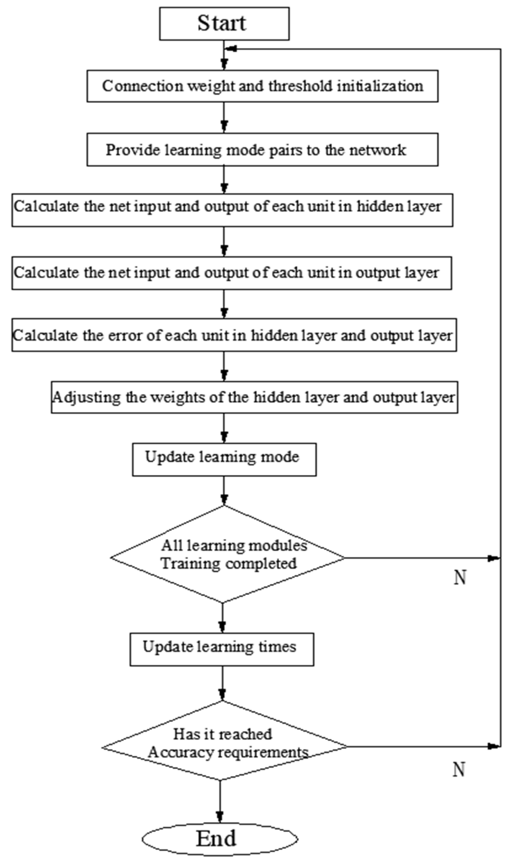
2.3. Evaluation Methods Based on Neural Networks

BP (backpropagation) artificial neural network is a multi-layer feedforward neural network based on an error backpropagation algorithm, mainly simulating the feedback behavior of neurons in the human brain in response to external signal stimuli. The BP artificial neural network has strong self-learning and self-regulation abilities. If it has training samples, it can construct nonlinear mapping relationships between various factors and has strong fault tolerance and robustness. The basic idea of using the BP artificial neural network method for evaluation is first to determine the structure of the BP artificial neural network and the number of neural nodes in each layer, therefore establishing a functional model of the BP artificial neural network. Then, we input learning sample data for cyclic learning training until the set learning accuracy is achieved, save the trained model, and input the indicator score matrix of the project to be evaluated to obtain the evaluation results [37].

The genetic algorithm (GA) was first proposed by John Holland in the United States in the 1970s. The algorithm was designed and proposed based on the evolutionary laws of organisms in nature [38]. It is a computational model that simulates the natural selection and genetic mechanisms of Darwin’s biological evolution theory and is a method of searching for optimal solutions by simulating the natural evolution process. This algorithm uses mathematical methods and computer simulation operations to transform the problem-solving process into a process similar to the crossover and mutation of chromosome genes in biological evolution. When solving complex combinatorial optimization problems, compared to some conventional optimization algorithms, they can usually achieve better optimization results quickly. Genetic algorithms have been widely applied in fields such as combinatorial optimization, machine learning, signal processing, adaptive control, and artificial life.

2.3.1. Criteria for Management Classification

According to the “Notice on Implementing the Comprehensive Implementation Plan for Standardized Management of Water Projects in Jiangxi Province” and relevant documents, the assessment and evaluation of standardized management for large and medium-sized reservoirs (locks) in Jiangxi Province are governed by the “Assessment and Evaluation Criteria for Standardized Management of Large and Medium-Sized Reservoirs (Locks) in Jiangxi Province” (referred to as the “Evaluation Criteria” hereafter).

The “Evaluation Criteria” adopts a scale of one thousand points, with a maximum evaluation score of 1000. Standardized management is classified into five levels based on the evaluation scores, with specific criteria as follows:

A score above 900 indicates a first-class evaluation level.

A score above 800 indicates a second-class evaluation level.

A score above 700 indicates a third-class evaluation level.

A score above 600 indicates a fourth-class evaluation level.

Scores below 600 are considered not to meet the standards.

2.3.2. Construction of the Evaluation Model

The input-output relationship of the BP artificial neural network represents a highly nonlinear mapping. If the number of input nodes is n and the number of output nodes is m, the network maps from an n-dimensional Euclidean space to an m-dimensional Euclidean space. By adjusting the connection weights and the network’s structure, including the number of hidden nodes, the BP artificial neural network can address nonlinear classification problems and approximate any nonlinear function with arbitrary precision. Once the structure of the BP artificial neural network is determined, training is performed using input-output sample sets. This involves learning and adjusting the network’s weights and thresholds to accurately express the given input-output mapping relationship. A trained BP artificial neural network can provide appropriate outputs even for inputs that were not part of the training set, demonstrating its generalization capability. From the perspective of function approximation, this indicates that the BP artificial neural network has interpolation functionality. The algorithm flow of the BP artificial neural network is shown in Figure 2.

3. Results

The case study process is as follows, and standardized management of the neural network evaluation model is shown in Figure 3.

The essence of the BP artificial neural network model is to find the global minimum points of a nonlinear function, which represents the error function. A given network model can have multiple local minimum points, so finding the global optimal solution requires changing the initial weights of the network multiple times and finding the corresponding local minimum points. By comparing these points, the minimum value can be determined, which represents the global optimal solution. Additionally, the performance of the network model can vary significantly depending on different parameters and network structures. Therefore, it is necessary to continuously adjust the parameters to compare the performance of different network models with different structures. A good neural network model refers to a network with a reasonable number of hidden layers and nodes, appropriate training, and no overfitting. The determination of the final model requires continuous parameter adjustment and result comparison.

3.1. Training Sample Selection

3.1.1. Preparation of Training Samples from Dike Data

It is known that the evaluation indicators consist of 2 levels. Among them, the first level of each category of dike projects contains 5 indicators, corresponding to management foundation, safety management, operation management, maintenance management, and management assurance. In the second-level indicators, dike engineering is divided into 44 sub-indicators (three-level indicators).

To determine the training data based on the weights of each indicator, it is generally required to have 5–10 times or 10–20 times the number of input variables as the training sample size for BP artificial neural networks. Using the random function round (rand (1, m) × X) in MATLAB (where m is the number of indicators and X is the weight vector of the indicators), 196 sets of simulated data are obtained for the simulation evaluation of the indicators, as shown in

Table 10. Sample set of network model training for dike engineering.

Indicator	1	2	3	4	5	6	7	8	$\cdots$	198	199	200
Pocket Book (D1)	1	0.9	1	0.98	1	1	0.98	1	$\cdots$	0.53	0.81	0.61
Management and Operations Manual (D2)	1	1	1	1	0.82	1	1	0.9	$\cdots$	0.75	0.67	0.68
Scope delineation (D3)	0.17	0.21	0.95	0.22	0.85	0.51	0.19	0.58	$\cdots$	0.5	0.93	0.11
Boundary Pile Embedding (D4)	0.88	0.83	1	0.81	1	1	1	0.93	$\cdots$	0.56	0.45	0.41
Number of identification plates (D5)	0.89	1	1	0.84	0.91	1	0.92	0.88	$\cdots$	0.61	0.6	0.8
Identification and Signage Category (D6)	1	0.84	0.95	1	1	1	1	1	$\cdots$	0.83	0.66	0.85
Archive facilities (D7)	1	1	1	1	1	1	1	0.84	$\cdots$	0.77	0.45	0.74
Data storage (D8)	1	1	0.92	0.85	0.93	0.95	1	0.82	$\cdots$	0.68	0.74	0.52
Responsible person implementation (D9)	1	1	1	1	1	1	1	1	$\cdots$	0.62	0.62	0.56
Safety inspection (D10)	0.72	1	1	0.6	0.68	0.55	0.77	1	$\cdots$	0.86	0.82	0.88
Safety equipment (D11)	0.58	0.52	0.47	0.85	1	0.69	0.87	0.97	$\cdots$	0.19	0.62	0.93
Work with certificate (D12)	0.68	0.86	1	0.66	0.83	1	0.55	0.92	$\cdots$	0.58	0.45	0.22
Emergency Plan (D13)	0.59	0.59	1	0.94	1	0.94	0.64	0.76	$\cdots$	0.54	0.26	0.43
Emergency drill (D14)	0.8	0.87	0.56	0.96	1	1	0.57	1	$\cdots$	0.44	0.89	0.67
Flood control materials (D15)	0.54	0.57	0.56	0.83	0.98	0.43	1	1	$\cdots$	0.36	0.87	0.36
Flood Control Traffic (D16)	0.97	1	0.82	1	1	0.95	1	0.85	$\cdots$	0.47	0.58	0.63
Flood Control Team (D17)	1	1	0.83	0.96	0.7	0.77	0.58	0.98	$\cdots$	0.73	0.78	0.46
Flood Control Duty (D18)	0.95	0.95	1	0.79	0.78	1	0.89	0.57	$\cdots$	0.6	0.33	0.33
Inspection frequency (D19)	1	1	0.92	1	1	1	1	0.92	$\cdots$	0.37	0.4	0.47
Inspection content (D20)	0.69	1	1	1	0.84	1	1	1	$\cdots$	0.56	0.56	0.52
Inspection Record (D21)	1	0.94	0.96	1	1	0.87	0.93	1	$\cdots$	0.65	0.51	0.47
Observation facility integrity rate (D22)	1	0.67	0.88	0.52	0.63	1	0.79	1	$\cdots$	0.53	0.59	0.6
Observation content and frequency (D23)	0.93	1	0.62	0.83	1	0.9	1	1	$\cdots$	0.76	0.82	0.72
Observation Record (D24)	1	1	0.95	1	0.98	0.98	1	1	$\cdots$	0.83	0.71	0.45
Operate according to chapter (D25)	1	1	1	1	1	0.84	0.93	1	$\cdots$	0.75	0.64	0.7
Operation Record (D26)	0.95	0.82	1	0.96	1	1	1	1	$\cdots$	0.85	0.69	0.48
Dike maintenance (D27)	0.76	0.89	0.94	1	0.68	0.73	0.91	0.77	$\cdots$	0.74	0.59	0.62
Piercing structures (D28)	1	1	1	1	1	1	0.86	1	$\cdots$	0.81	0.64	0.49
Prevention and control measures (D29)	1	1	1	1	1	1	1	1	$\cdots$	0.58	0.48	0.54
Maintenance Record (D30)	1	1	1	0.95	1	0.95	0.88	1	$\cdots$	0.38	0.66	0.56
Metal structure (D31)	0.88	1	1	1	1	1	0.91	1	$\cdots$	0.71	0.73	0.85
Mechanical and Electrical Equipment (D32)	1	1	1	1	1	0.92	1	0.99	$\cdots$	0.5	0.79	0.78
Maintenance Record (D33)	0.88	1	0.87	1	1	1	1	0.89	$\cdots$	0.65	0.71	0.52
Embankment Appearance (D34)	0.86	0.98	1	1	1	0.91	0.99	0.9	$\cdots$	0.61	0.43	0.46
Office area (D35)	1	1	0.9	0.81	0.9	1	0.91	1	$\cdots$	0.46	0.72	0.7
Job Setting (D36)	1	0.92	0.89	1	1	0.91	1	1	$\cdots$	0.79	0.45	0.83
Education and Training (D37)	1	1	1	1	0.96	1	1	1	$\cdots$	0.38	0.44	0.81
Video surveillance (D38)	1	1	1	1	1	1	1	1	$\cdots$	0.52	0.67	0.62
Platform Construction (D39)	1	1	1	0.96	1	1	1	0.81	$\cdots$	0.66	0.64	0.68
Platform Operation and Maintenance (D40)	0.83	0.9	1	1	0.99	1	1	1	$\cdots$	0.7	0.75	0.65
Management self-assessment (D41)	0.9	0.93	0.97	1	1	1	0.92	1	$\cdots$	0.47	0.41	0.6
Reward and Punishment Hook (D42)	0.48	0.1	0.22	0.97	0.01	0.56	0.67	0.88	$\cdots$	0.53	0.92	0.77
Budget (D43)	1	1	1	0.85	1	1	1	1	$\cdots$	0.8	0.4	0.62
Fund availability rate (D44)	0.99	1	1	1	1	1	1	1	$\cdots$	0.48	0.46	0.81
Desired output	0.89	0.91	0.91	0.93	0.90	0.91	0.91	0.93		0.60	0.61	0.58

. In addition, to improve the robustness of the network, 4 additional data sets are artificially added, representing the critical values of each indicator.

Through comparative analysis and expert judgment of the evaluation indicators for various types of engineering management, the expert evaluation values of the samples are calculated. The comprehensive evaluation values obtained using the AHP method are used here. Finally, the training data and the comprehensive evaluation values are saved in an Excel spreadsheet as an import file (xls). The first row represents the data index, the last row represents the comprehensive evaluation values, the first column represents the indicator names, and columns 1 to 200 are reserved for data storage.

3.1.2. Data Preprocessing

To improve the fitting effect of the model, the first step is to discretize all the indicators. Since the second-level indicators are qualitative, no further discretization is required. The main focus is on type normalization and dimensionless processing of the data, transforming all input and output data to the range of 0 to 1. The reason for data normalization is that the BP artificial neural network commonly deals with nonlinear functions, and the nonlinear process is implemented by the activation function of the network. The sigmoid function is the most commonly used activation function, with a value range of [0, 1]. Without data normalization, there may be significant differences in the magnitude of the data, where smaller values correspond to smaller errors, and larger values correspond to larger errors. As mentioned earlier, the training process of the BP artificial neural network adjusts the network weights based on the total error. Without data normalization, components with smaller errors will have a larger proportion of the total error than components with larger errors. This can be detrimental to the optimization of the network within a certain number of iterations. Data normalization effectively reduces the impact of this issue on the accuracy of the model, which has been proven by many researchers.

Data normalization can be done using the maximum-minimum method or the mean-variance method. In this paper, the maximum-minimum method is used, and the function is defined in Equation (6).

$$y=\left(y_{\max }-y_{\min }\right)\times \left(x_k-x_{\min }\right)/\left(x_{\max }-x_{\min }\right)+y_{\min }$$

(6)

The equation is defined as follows: y_max and y_min are parameters that can be set by the user, with a default value of −1 and 1, respectively. $x_k$ represents the k-th indicator value. $x_{\min }$ and $x_{\max }$ is the minimum number and the maximum number in the data sequence. y represents the normalized value.

Similarly, the output values are also normalized and transformed to values between 0 and 1.

3.2. Determination of Network Topology Structure

The determination of network topology structure is crucial for ensuring the objectivity, accuracy, and applicability of the evaluation results in the BP artificial neural network model. It is one of the key focuses in establishing the model. The determination of network topology structure includes several aspects: the number of network layers, the number of nodes in the input layer, the number of hidden layers, the number of nodes in each hidden layer, and the number of nodes in the output layer.

3.3. Determination of Network Layers

The number of hidden layers in the BP artificial neural network model has been subject to theoretical research by many scholars. Hecht Nielsen has proven that when each node has different thresholds, a continuous function within a closed interval can be approximated by a network with a single hidden layer. A three-layer network can achieve arbitrary n-dimensional to m-dimensional mapping. Research in relevant literature suggests that compared to BP artificial neural network models with only one hidden layer, networks with two hidden layers are more prone to local minima and are more difficult to train. Therefore, for the establishment of the standardization management evaluation, the network model consists of an input layer, a hidden layer, and an output layer.

3.4. Determination of Input Layer Nodes

The number of input layer nodes is determined by the nature of the actual problem that the model needs to solve. For the standardization management evaluation problem, the indicator system used in this study consists of 18 influencing factors. These factors can comprehensively reflect the management status of a project and are commonly chosen as evaluation criteria for most water resources engineering management evaluations. Therefore, the input layer of the established standardization management evaluation network model contains 18 input nodes.

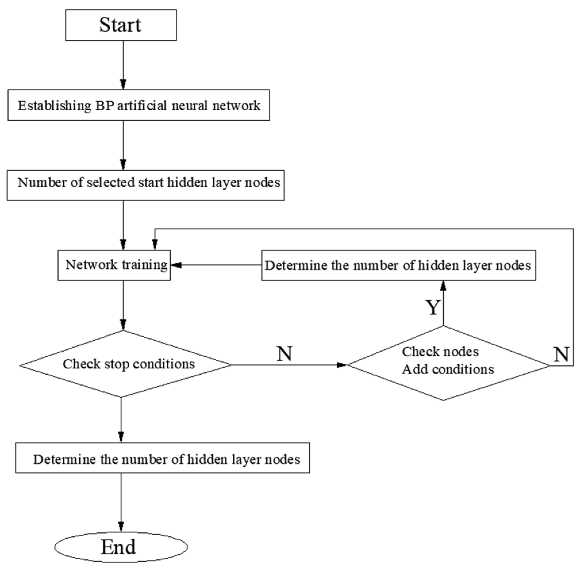
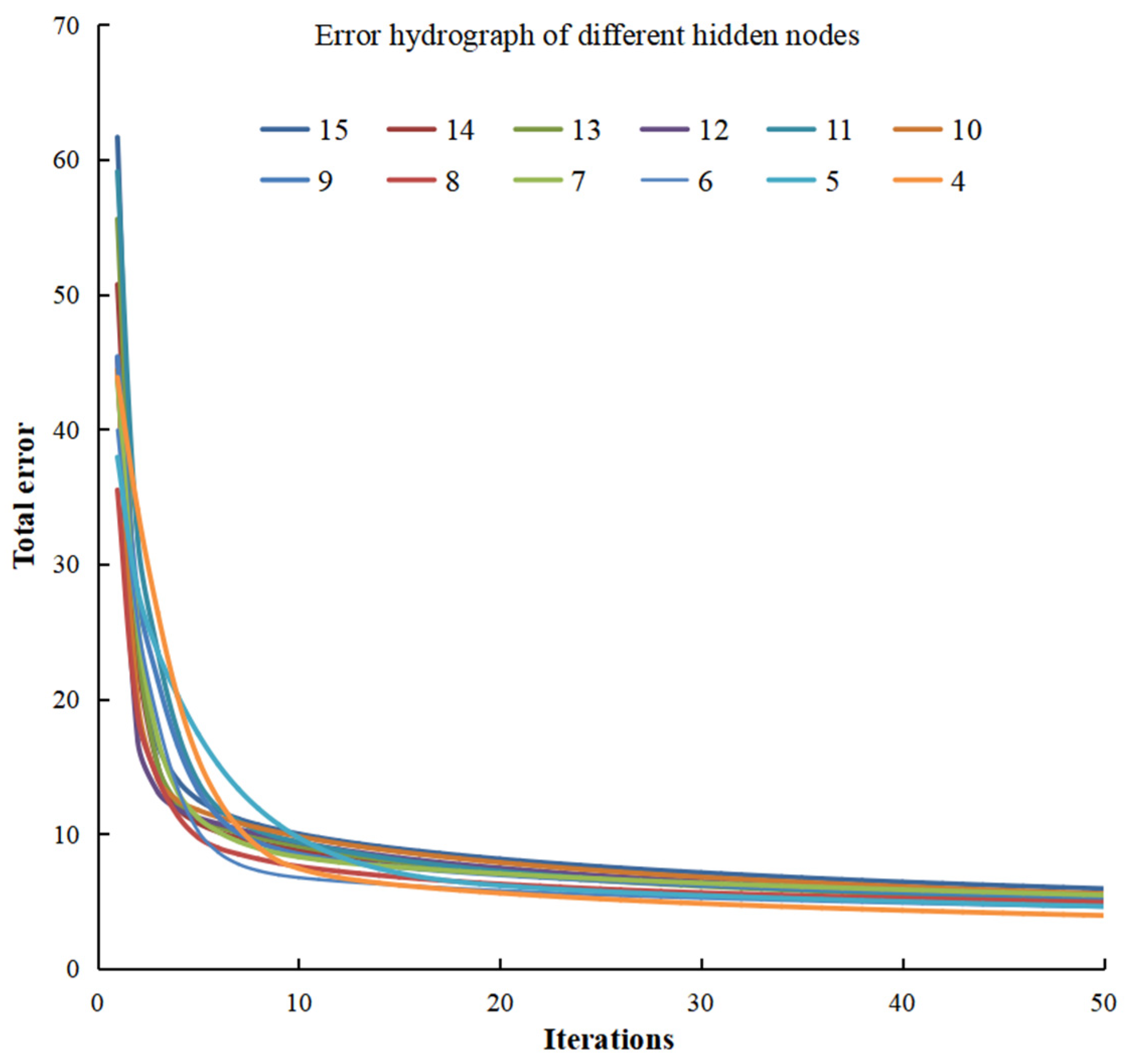
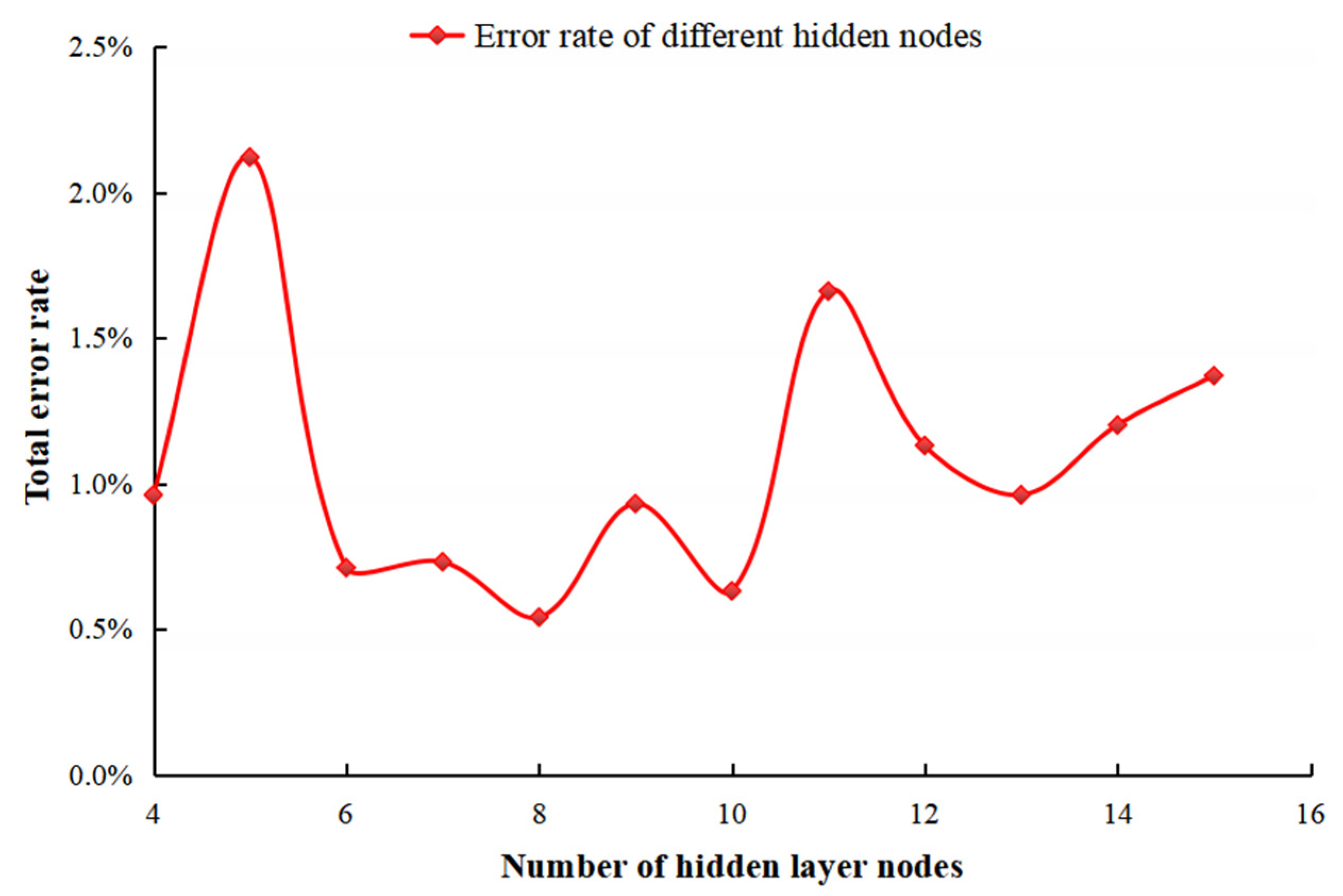
3.5. Determination of Hidden Layer Nodes

To determine the number of hidden layer nodes, the node growth method is used in this paper. The node growth method starts with the smallest neural network structure as a starting point and continuously increases the number of nodes until a satisfactory number is reached. This method of node splitting is also known as cell division. Refer to Figure 4 for a detailed illustration of the specific procedure.

In this project, the BP artificial neural network is established with 18 nodes in the input layer, 1 node in the output layer, and a total of 200 training samples. The number of hidden layer nodes is determined using the node growth method. Initially, the number of hidden layer nodes is set to 5, and through iterative trials, the optimal number of hidden layer nodes for this model is determined.

3.6. Analysis of the BP Artificial Neural Network Model

MATLAB provides a built-in computational tool for neural networks called “newff”. However, using this tool makes it difficult to obtain hidden parameters such as weight values, reduces optimization flexibility, and is less suitable for later system development. Therefore, in this study, a custom BP artificial neural network code was developed in the MATLAB environment. The results of the computational analysis of dike engineering are as follows:

Figure 5 shows the variation of the total training sample error with different numbers of hidden nodes. Overall, the trend of the curves is similar. The error rapidly decreases in the initial phase and then levels off, eventually converging. However, at a local level, the speed of descent varies among different curves. In the range of 11 to 15 hidden nodes and 4 to 6 hidden nodes, the curves start at a higher position and converge relatively slowly. On the other hand, when the number of hidden nodes is in the range of 7 to 9, the convergence speed is faster, and the total error is relatively smaller, resulting in better prediction performance. The total error after convergence falls between 5% and 7%, with an average error of approximately 2%.

Figure 6 shows the error rate curves for different numbers of hidden nodes. The curves exhibit a concave parabolic distribution with higher error rates on both ends and lower rates in the middle. Specifically, when the number of hidden nodes is 8, the error rate is at its lowest, only 0.5%. However, for numbers above 10, the error rate ranges between 1% and 2%.

In Figure 7, in the case of the optimal number of hidden nodes, it can be observed that the output error value falls below 0.00001 after 300 iterations, meeting the desired accuracy requirement, and the computation is terminated.

Table 11. Error rates for dike engineering.

Sample Serial Number	1	2	3	4	5	6	7	8	9	10
Desired output	0.602	0.679	0.795	0.919	0.721	0.826	0.908	0.854	0.828	0.658
Actual output	0.600	0.666	0.786	0.923	0.732	0.859	0.897	0.850	0.822	0.657
Error	−0.002	−0.013	−0.008	0.004	0.011	0.034	−0.011	−0.004	−0.006	−0.001
Error rate	0%	−2%	−1%	0%	2%	4%	−1%	0%	−1%	0%
Sample Serial Number	11	12	13	14	15	16	17	18	19	20
Desired output	0.853	0.576	0.899	0.928	0.691	0.704	0.922	0.695	0.553	0.588
Actual output	0.853	0.565	0.890	0.925	0.688	0.717	0.906	0.685	0.541	0.580
Error	0.001	−0.011	−0.009	−0.004	−0.003	0.013	−0.016	−0.010	−0.012	−0.008
Error rate	0%	−2%	−1%	0%	0%	2%	−2%	−1%	−2%	−1%

presents the validation results of 20 test data points. The error rates for each measurement point are relatively small, except for sample number 11, which has an error of 3%. The errors for the other samples are generally around 2%, with an average error of 1.2%. This indicates the good feasibility of the model, with the errors meeting the evaluation requirements. Using the built-in neural network tool “newff” in MATLAB and inputting the training data for analysis, the calculated average error is around 2%, slightly higher than the results obtained from the custom code developed in this study. This suggests that the code developed in this study is scientifically reasonable and meets the expected requirements.

4. Discussion

4.1. Optimization of Initial Weights

In neural networks, random initial weights are assigned, which can result in slightly different final weights and training iterations. This lack of uniqueness in weight optimization may lead to local minima, where the network converges to a local optimal solution instead of a global optimal solution. Randomly assigning initial weights can also result in excessive training iterations, slow convergence, and low efficiency. Additionally, there is greater uncertainty in the evaluation conclusions of neural network models, as the same input can yield different levels of accuracy.

Basic approach: ① Establish an improved BP artificial neural network using all training samples and encode the connection weights of the improved network to generate an initial population. ② Utilize a genetic algorithm to optimize the initial population and define a superior search space in the solution space. Optimize the weights of the improved BP artificial neural network during this process. ③ Use the decoded solutions from the genetic algorithm optimization as the initial weights of the improved BP artificial neural network to establish the nonlinear mapping relationship from input to output. ④ Utilize the trained network to evaluate the modernization level of water conservancy engineering management in the evaluated area.

Implementation steps:

• Chromosome Encoding and Population Encode the data to determine the chromosome. In this study, real number encoding is used, directly using the connection weights as the chromosome for encoding. For the 3-layer BP artificial neural network established, the chromosome can be represented by a set of weights, denoted as W in Equation (7).

  $$W_i=\{{\omega }_i{}_j,{\omega }_{jk},b_j,b_k\}$$

  (7)

  In the equation, ${\omega }_i{}_j$ represents the weights from the input layer to the hidden layer; ${\omega }_{jk}$ represents the weights from the hidden layer to the output layer; $b_j$ represents the output threshold of the hidden layer, and $b_k$ represents the output threshold of the output layer.
  The initial population is generated randomly using the small interval generation method. This involves dividing the range of values for the parameters to be optimized into smaller intervals equal to the total population size. Then, within each interval, a random individual is generated, forming the initial population.
• Fitness Function. The fitness function calculates the absolute difference between the predicted values and the actual values, sums them up, and takes the reciprocal. The formula is as follows in Equation (8):

  $$\mathrm{F}=1/(\sum _{\mathrm{i}=1}^{\mathrm{n}}\mathrm{a}\mathrm{b}\mathrm{s}(y_i-a_i))$$

  (8)

  In the equation, y_i represents the actual value, a_i represents the predicted value, and n represents the number of output nodes.
• Selection Operator. The selection operator utilizes a random sampling method and the best preservation strategy, with the main objective of identifying the best individuals in the population. However, selecting only the best individuals may overlook the diversity of the rest of the population, leading to local optima. To address this, each generation’s population is sorted based on fitness in ascending order. Then, the individuals are divided into segments using the ratios of 0.6, 0.8, and 1. From the end of each segment, individuals are randomly sampled to compensate for the potential loss of diversity. This approach maintains both global convergence characteristics and population diversity.
• Crossover Operation. Crossover involves selecting two individuals from the population and performing crossover at certain positions with a certain probability of generating new individuals. Since real number encoding is used in this study, real number crossover is applied. Specifically, at the i-th position, a crossover is performed between the m-th chromosome (a_m) and the n-th chromosome (a_n) in Equation (9):

  $$\left\{\begin{array}{c}{a}_{mi}=a_{mi}\left(1-b\right)+a_{ni}b\\ a_{ni}=a_{ni}\left(1-b\right)+a_{mi}b\end{array}\right.)$$

  (9)

  In the equation, b represents a random number between 0 and 1.
• Mutation Operation. Mutation is the process of randomly selecting an individual and applying mutation to its chromosome with a certain probability of generating a new individual. The method is shown in Equation (10):

  $$a_{mn}=\left\{\begin{array}{c}{a}_{mn}+{(a}_{mn}-a_{max})\times f\left(g\right),r>0.5\\ a_{mn}+{(a}_{min}-a_{mn})\times f\left(g\right),r\le 0.5\end{array}\right.$$

  (10)

  In the equation, the upper bound of the gene a_mn is a_max, and the lower bound is a_min. $f\left(g\right)=r_2(1-g/G_{max})$, where g is the current iteration count, G_max is the maximum evolution count, r is a random number between 0 and 1, and r₂ is another random number.
• Apply the chromosome to the neural network, calculate the fitness, and analyze if the set requirements are met. If the requirements are satisfied, decode the optimal individual as the optimal initial weights of the BP artificial neural network and proceed to the next step. Otherwise, go to step 3.
• Set the learning rate n, momentum coefficient m, allowable error c, and maximum training count N for BP artificial neural network as part of the loop step I.
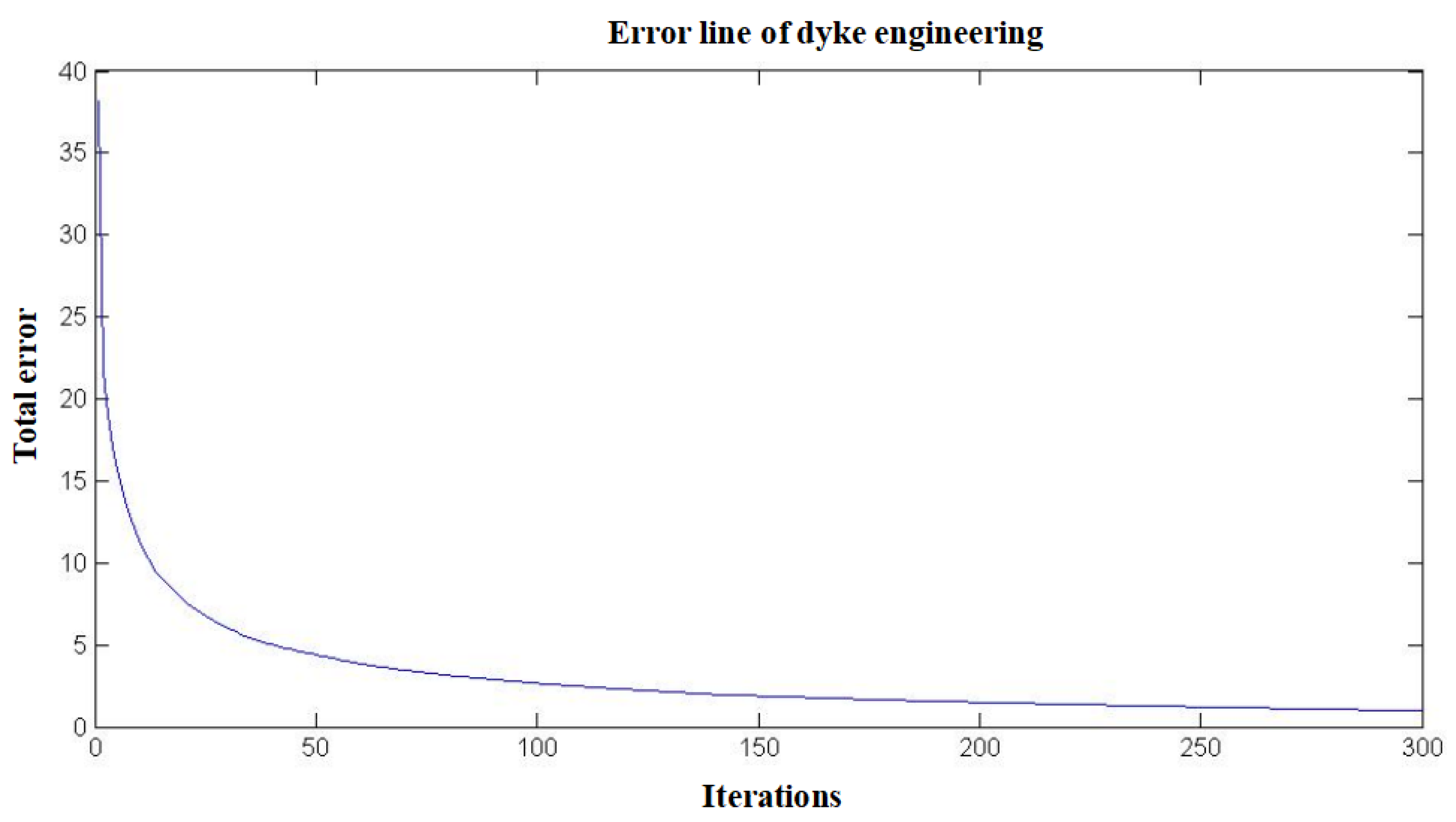
• Input the normalized samples into the network, train the BP artificial neural network by adjusting the network weights, and calculate the network output and total error E.
• If E ≤ e (the desired training accuracy), then training is complete, and proceed to the next step. Otherwise, take the optimized connection weights from this iteration as the initial weights for the next training. Adjust the network weights and biases and go to step 7.
• Output the network connection weights that meet the training accuracy requirement (i.e., E ≤ e).
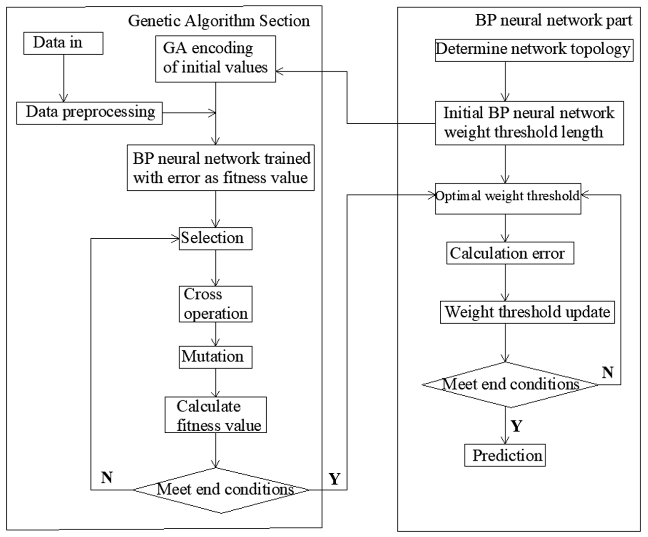
• Evaluate the standardized management level of the water conservancy project for the evaluated object and calculate the evaluation results. The program flow of the GA-BP artificial neural network evaluation algorithm for improving the modernization of water conservancy project management is shown in Figure 8.

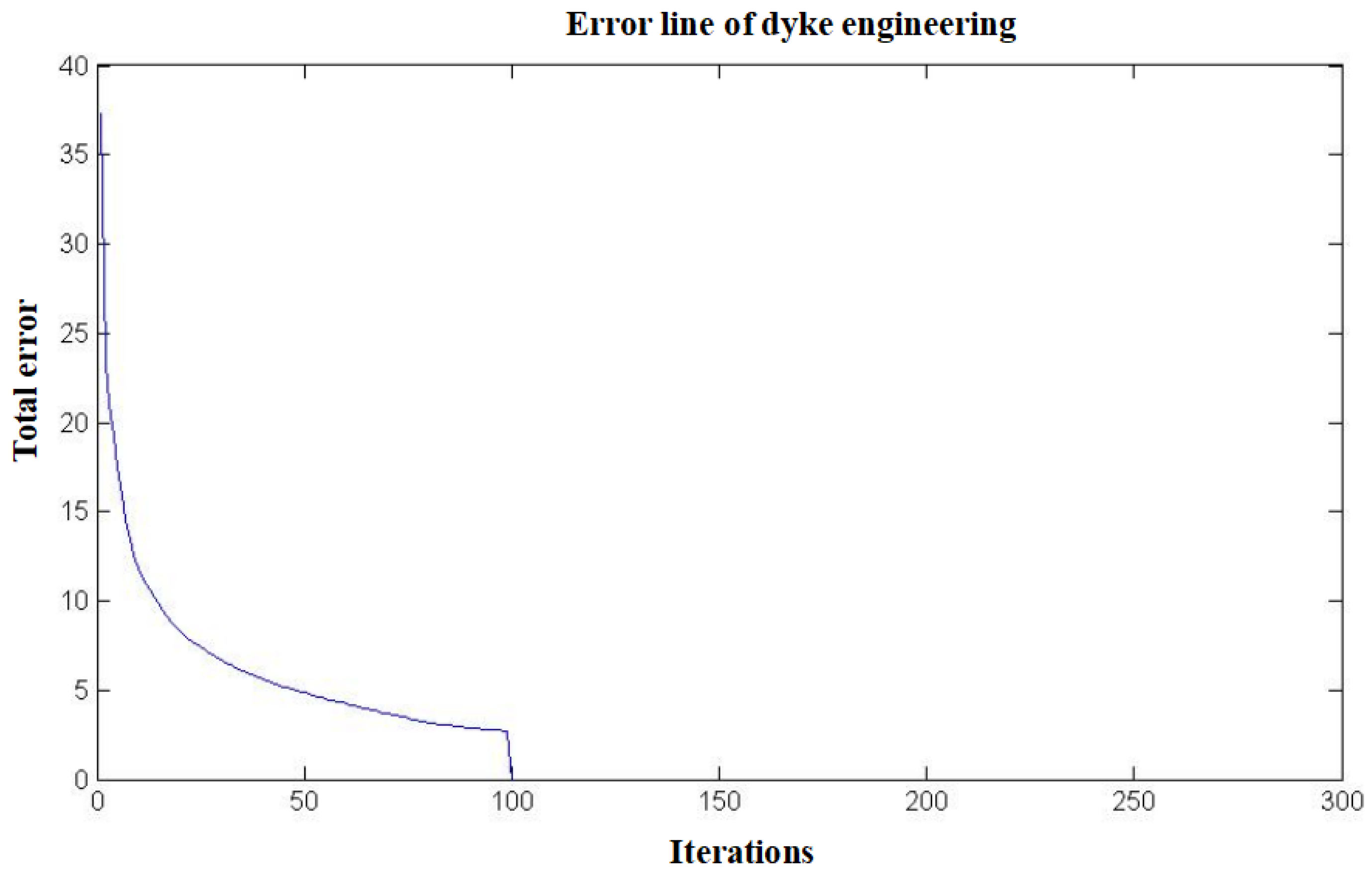
4.2. GA-BP Network Model Computational Analysis

In the GA-BP model algorithm, the crossover probability is set to 0.7, the mutation probability is set to 0.2, and the population size is set to 10.

As shown in Figure 9 for dike engineering, the error curve decreases rapidly, and the desired accuracy is achieved in approximately 100 iterations, leading to the termination of the computation. The GA-BP model demonstrates faster computation speed compared to the BP artificial neural network model.

In terms of computational accuracy, as shown in

Table 12. Error rates for dike engineering.

Sample Serial Number	1	2	3	4	5	6	7	8	9	10
Desired output	0.811	0.738	0.679	0.922	0.840	0.613	0.614	0.607	0.793	0.676
Actual output	0.801	0.721	0.676	0.916	0.830	0.603	0.597	0.612	0.787	0.664
Error	−0.01	−0.02	0.00	−0.01	−0.01	−0.01	−0.02	0.00	−0.01	−0.01
Error rate	−1.3%	−2.4%	−0.5%	−0.7%	−1.3%	−1.6%	−2.8%	0.8%	−0.7%	−1.7%
Sample Serial Number	11	12	13	14	15	16	17	18	19	20
Desired output	0.562	0.900	0.871	0.595	0.730	0.897	0.897	0.687	0.693	0.556
Actual output	0.567	0.903	0.861	0.592	0.743	0.881	0.884	0.693	0.702	0.569
Error	0.00	0.00	−0.01	0.00	0.01	−0.02	−0.01	0.01	0.01	0.01
Error rate	0.9%	0.4%	−1.2%	−0.5%	1.9%	−1.8%	−1.4%	1.0%	1.3%	2.3%

, the errors for each sample are relatively small, generally within 1%. The average error is 1.3%, which is an improvement compared to the BP neural network model. This indicates that an improved evaluation model is more reasonable and capable of performing evaluations.

5. Conclusions

This research constructed an evaluation index system. Based on the existing evaluation index system, it analyzed the principles and methods for determining evaluation indicators for the main type of engineering projects, namely dikes. The evaluation indicators were divided into three levels, and the hierarchical structure of the index system was clear, facilitating normalized management.

This research used the Analytic Hierarchy Process (AHP) to determine weights. Based on expert knowledge and subjective experience, it used mathematical methods to remove subjective components as much as possible and calculated the weights of the indicators. This approach made the weights more in line with objective reality and easier to quantify, therefore improving the reliability, accuracy, and objectivity of the evaluation.

This research studied the technical methods of artificial neural networks in hydraulic engineering management evaluation. By incorporating momentum factors and adaptive learning rates for improvement and coupling genetic algorithms with modified backpropagation algorithms, it enhanced the search speed and accuracy of the neural network algorithm. Combining the characteristics of modernized management evaluation in hydraulic engineering, it calibrated relevant parameters, established the improved GA-BP evaluation algorithm, and applied this algorithm to hydraulic engineering management evaluation for the first time. The evaluation results demonstrated that this method better reflects the importance of maintenance management and operation management.

Based on the MATLAB platform, this research developed the code for the improved GA-BP evaluation algorithm, which can be further integrated into the Jiangxi Province Hydraulic Engineering Operation Management Information System. The evaluation of hydraulic engineering management is based on the standardized management evaluation in our province. It conducted research on the evaluation methods, selection of evaluation indicators, and assignment of indicator weights within a systematic framework. The various components of the entire system are interconnected, aiming to establish mathematical models, evaluation steps, and corresponding practical techniques. The fuzzy comprehensive evaluation method based on the Analytic Hierarchy Process and the application of neural network methods in evaluation have broad application prospects and high promotion value.

The standardized management of water conservancy engineering is still in its infancy in China, and the working methods and technical requirements will continue to improve with the progress of time. Based on absorbing advanced management experience, this project actively introduces advanced AHP comprehensive evaluation technology and neural network technology, forming its own unique standardized management evaluation method. Given the limited conditions, the results have not yet been widely applied, and the understanding of standardized management needs to be improved. In the future, we hope to conduct more in-depth research to make the results more reasonable and feasible. For example, standardized management of water conservancy engineering is a large-scale project that involves a wide range of aspects. How to better establish a standardized management system in our province based on existing work achievements and provide a structurally sound, reasonable, and feasible theoretical basis is an effective measure to promote standardized management in a normalized manner. Establishing a more comprehensive and clear standardized management evaluation index system is an important content. Establishing a realistic evaluation model requires repeated practice and continuous improvement, which is a “learning” process. In the future, the achievements of standardized management in water conservancy engineering should be widely utilized to conduct multi-level and multi-angle research and evaluate the effectiveness of this evaluation model. In addition, we will actively try other methods that could be used (TOPSIS, SIMUS, SAW, PROMETHEE, etc.).

References

1. Qu, J.; Meng, X.; You, H. Multi-stage ranking of emergency technology alternatives for water source pollution accidents using a fuzzy group decision making tool. J. Hazard. Mater. 2016, 310, 68–81. [Google Scholar] [CrossRef]
2. Tu, W.R.; Fang, S.B.; Sun, Z.L. Experimental study and flow analysis on a new design of water-retaining sluice gate. Water Pract. Technol. 2020, 15, 311–320. [Google Scholar] [CrossRef]
3. Wang, D.; Li, Y.; Yang, X.; Zhang, Z.; Gao, S.; Zhou, Q.; Zhuo, Y.; Wen, X.; Guo, Z. Evaluating urban ecological civilization and its obstacle factors based on integrated model of PSR-EVW-TOPSIS: A case study of 13 cities in Jiangsu Province, China. Ecol. Indic. 2021, 133, 108431. [Google Scholar] [CrossRef]
4. Wang, Q.; Li, S.; Li, R. Evaluating water resource sustainability in Beijing, China: Combining PSR model and matter-element extension method. J. Clean. Prod. 2019, 206, 171–179. [Google Scholar] [CrossRef]
5. Lea, D.A.; Löffler, E.; Douglas, I. Review symposium: Our common future: The world commission on environment and development. Aust. Geogr. 1989, 20, 195–201. [Google Scholar] [CrossRef]
6. Gunhan, S. Analyzing Sustainable Building Construction Project Delivery Practices: Builders’ Perspective. Pract. Period. Struct. Des. Constr. 2019, 24, 05018003. [Google Scholar] [CrossRef]
7. Sharifi, A.; Murayama, A. A critical review of seven selected neighborhood sustainability assessment tools. Environ. Impact Assess. Rev. 2013, 38, 73–87. [Google Scholar] [CrossRef]
8. Feng, H.; Hewage, K. Energy saving performance of green vegetation on LEED certified buildings. Energy Build. 2014, 75, 281–289. [Google Scholar] [CrossRef]
9. Koskela, L. Lean Productionin Construction. In Lean Construction; Elsevier Science Publishers R.V.: Amsterdam, The Netherlands, 1992; Volume 12, pp. 241–249. [Google Scholar]
10. Nahmens, I. From lean to green construction: A natural extension. In Proceedings of the Building a Sustainable Future—Proceedings of the 2009 Construction Research Congress, Seattle, WA, USA, 5–7 April 2009; pp. 1058–1067. [Google Scholar]
11. Du Plessis, C. Astrategic framework for sustainable construction in developing countries. Constr. Manag. Econ. 2007, 25, 67–76. [Google Scholar] [CrossRef]
12. Marhani, M.A.; Jaapar, A.; Bari, N.A.A. Lean Construction: Towards enhancing sustainable construction in Malaysia. Procedia-Soc. Behav. Sci. 2012, 68, 87–98. [Google Scholar] [CrossRef]
13. Circo, C.J. Using Mandatesand Incentivesto Promote Sustainable Construction and Green Building Projects in the Private Sector: A Call for More State Land Use Policy Initiatives. Ph.D. Thesis, University of Arkansas, Faye-Tteville, NC, USA, 2008. [Google Scholar]
14. Robichaud, L.B.; Anantatmula, V.S. Greening Project Management Practices for Sustainable Construction. J. Manag. Eng. 2010, 27, 48–57. [Google Scholar] [CrossRef]
15. Choi, K.; Lee, H.W. Environmental, Economic, and Social Implications of Highway Concrete Rehabilitation Altematives. J. Constr. Eng. Manag. 2016, 142, 04015079. [Google Scholar] [CrossRef]
16. Kokkaew, N.; Rudjanakanoknad, J. A Framework of Green Growth Assessment for Thailand’s Highway Infrastructure Developments. In Computing in Civil and Building Engineering; ASCE: Reston, VA, USA, 2014; pp. 1951–1959. [Google Scholar]
17. Wang, S.-J. Bionic (topological) pattern recognition -A new model of pattern recognition theory and its applications. Acta Electron. Sin. 2002, 30, 1417–1420. [Google Scholar]
18. Zhou, Z.H.; Jiang, Y.; Chen, S.F. Extracting symbolic rules from trained neural networks ensembles. AI Commun. 2003, 16, 3–15. [Google Scholar]
19. Liao, X.F.; Wong, K.W.; Wu, Z.F.; Chen, G.R. Novel robust stability criteria for interval-delayed Hopfield neural networks. IEEE Trans. Circuits Syst. 2001, 48, 1355–1359. [Google Scholar] [CrossRef]
20. Liao, X.F.; Chen, G.R.; Sanchez, E.N. LMI-based approach for asymptotically stability analysis of delayed neural networks. IEEE Trans. Circuits Syst. 2002, 49, 1033–1039. [Google Scholar] [CrossRef]
21. Liao, X.F.; Wong, K.W.; Yu, J.B. Novel stability condition for cellular networks with time delay. Int. J. Bifurc. Chaos 2001, 11, 1853–1864. [Google Scholar] [CrossRef]
22. Ni, S.; Bai, Y. Application of BP neural network model in groundwater water quality evaluation. Syst. Eng. Theory Pract. 2000, 20, 124–127. [Google Scholar]
23. Zhu, Q.; Zhang, G. Evaluation model of enterprise knowledge management based on artificial neural network. Stud. Sci. Sci. 2003, 8, 32–34. [Google Scholar]
24. Wang, M. Improvement and application of BP neural network algorithm. Comput. Eng. Appl. 2009, 35, 47–48. [Google Scholar]
25. Yan, B.; Gao, Z.; Li, D. Application of RBF neural network in comprehensive safety evaluation of dams. Chin. J. Rock Mech. Eng. 2008, 23, 3991–3997. [Google Scholar]
26. Wang, A.; Sun, J. Application of BP neural network in engineering project management. Mod. Build. Manag. 2009, 23, 306–309. [Google Scholar]
27. Bashiri, M.; Badri, H.; Hejazi, T.H. Selecting optimum maintenance strategy by fuzzy interactive linear assignment method. Appl. Math. Model. 2011, 35, 152–164. [Google Scholar] [CrossRef]
28. Ali, A.; Zhu, Y.; Zakarya, M.J.N. Exploiting dynamic spatio-temporal graph convolutional neural networks for citywide traffic flows prediction. Neural Netw. 2022, 145, 233–247. [Google Scholar] [CrossRef] [PubMed]
29. Yan, D.; Zhang, H.; Li, G.; Li, X. Improved method to detect the tailings ponds from multispectral remote sensing images based on faster R-CNN and transfer learning. Remote Sens. 2022, 14, 103. [Google Scholar] [CrossRef]
30. Li, Y.; Bao, T.; Gao, Z.; Shu, X.; Zhang, K.; Xie, L.; Zhang, Z. A new dam structural response estimation paradigm powered by deep learning and transfer learning techniques. Struct. Health Monit.-Int. J. 2022, 21, 770–787. [Google Scholar] [CrossRef]
31. Dong, L.; Deng, S.; Wang, F. Some developments and new insights for environmental sustainability and disaster control of tailings dam. J. Clean. Prod. 2020, 269, 122270. [Google Scholar] [CrossRef]
32. Jia, T.; Wang, R.; Chai, B. Effects of heavy metal pollution on soil physicochemical properties and microbial diversity over different reclamation years in a copper tailings dam. J. Soil Water Conserv. 2019, 74, 439–448. [Google Scholar] [CrossRef]
33. Cheng, M.Y.; Cao, M.T.; Huang, I.F. Hybrid artificial intelligence-based inference models for accurately predicting dam body displacements: A case study of the Fei Tsui dam. Struct. Health Monit.-Int. J. 2022, 21, 1738–1756. [Google Scholar] [CrossRef]
34. Chen, H.; Li, H.; Wang, Y.; Cheng, B. A Comprehensive Assessment Approach for Water-Soil Environmental Risk during Railway Construction in Ecological Fragile Region Based on AHP and MEA. Sustainability 2020, 12, 7910. [Google Scholar] [CrossRef]
35. Ikram, M.; Sroufe, R.; Zhang, Q. Prioritizing and overcoming barriers to integrated management system (IMS) implementation using AHP and G-TOPSIS. J. Clean. Prod. 2020, 254, 120121. [Google Scholar] [CrossRef]
36. Darko, A.; Chan AP, C.; Ameyaw, E.E.; Owusu, E.K.; Pärn, E.; Edwards, D.J. Review of application of analytic hierarchy process (AHP) in construction. Int. J. Construct. Manag. 2019, 19, 436–452. [Google Scholar] [CrossRef]
37. Barcelos, D.A.; Pontes, F.V.; da Silva, F.A.; Castro, D.C.; Dos Anjos, N.O.; Castilhos, Z.C. Gold mining tailing: Environmental availability of metals and human health risk assessment. J. Hazard. Mater. 2020, 397, 122721. [Google Scholar] [CrossRef] [PubMed]
38. Belmokre, A.; Mihoubi, M.K.; Santillan, D.J. Seepage and dam deformation analyses with statistical models: Support vector regression machine and random forest. Procedia Struct. Integr. 2019, 17, 698–703. [Google Scholar] [CrossRef]
Figure 1. Distribution Map of Water Conservancy Projects in Jiangxi Province (On the left is a map of China, and on the right is a distribution map of dike in Jiangxi Province).
Water 15 03713 g001
Figure 2. Flow chart of the BP learning algorithm.
Water 15 03713 g002
Figure 3. Standardized management of the neural network evaluation model.
Water 15 03713 g003
Figure 4. Flowchart for hidden node selection in the node growth method.
Water 15 03713 g004
Figure 5. Total error of the training samples.
Water 15 03713 g005
Figure 6. Error rates for different numbers of hidden nodes.
Water 15 03713 g006
Figure 7. Error line of dike engineering.
Water 15 03713 g007
Figure 8. Water standardized management improved the GA-BP evaluation algorithm.
Water 15 03713 g008
Figure 9. Dike evaluation results using the improved BP model.
Water 15 03713 g009