Experimental Research on Ice Density Measurement Method Based on Ultrasonic Waves

Abstract

Ice density is an important physical parameter affecting the mechanical properties of ice. Due to bad field environments, the traditional density measurement method cannot achieve continuous monitoring of ice density. Therefore, the authors of this paper propose a new idea: to use the acoustic characteristics of ice to obtain ice density. The acoustic and physical properties of artificially frozen ice samples, with salinity values in the range of 0~8.5‰, were tested using a nonlinear high-energy ultrasonic testing system to explore the relationships among ice density, sound velocity, temperature, and salinity when the temperatures of the ice samples rose from −30 °C to −5 °C. The test results show that the freshwater ice density decreases from 915.5 kg/m³ to 911.9 kg/m³ when the ice temperature rises from −30 °C to −5 °C. The density of saltwater ice varies from 899.8 kg/m³ to 912.9 kg/m³. When the salinity remains the same, the density of an ice sample decreases with an increase in temperature and increases with an increase in sound velocity. When the ice temperature remains the same, the density of saltwater ice increases with an increase in salinity and decreases with an increase in sound velocity. Based on the test results, a prediction model of ice density with respect to sound velocity, temperature, and salinity is established. The root mean square error between the predicted values of the model and the measured values is 0.337 kg/m³, indicating that the prediction accuracy is high.

1. Introduction

As an important load for hydraulic design in cold regions, ice is prone to expansion and drift due to environmental factors, causing extrusion and impacts on marine platforms and seriously threatening the safety of hydraulic buildings [1,2,3]. Ice also affects marine traffic and shipping, blocking the development of marine resources and the aquaculture industry and causing serious economic losses. Ice thickness and mechanical properties are the main indicators of changes in ice conditions, and research on the physical and mechanical properties of ice is extremely important for the maintenance of hydraulic structures and for the opening of waterways. As an important engineering parameter, ice density is not only an important input parameter in the inversion of ice thickness using a satellite altimeter [4], but it also plays a key role in testing for the determination of the mechanical properties of ice [5]. For remote sensing observations of ice thickness, an uncertainty of about ±4% in the measurement of ice density may result in an inversion error of about ±30% for one year of sea ice with a thickness of 1.1–2.0 m [6]. Therefore, accurately obtaining information on ice density and its changes is the key to analysing changes in ice conditions on water.

The process of ice growth may result in the formation of non-linear crystals, which are generally classified as granular and columnar ice. When ice freezes rapidly, granular ice is formed. After the ice growth rate decreases, the crystals have enough time to grow, but the sides of the ice crystals are gradually occupied by other crystals, which can only grow vertically downwards to form columnar crystals [7]. Since these two crystal structures are too complex, only regular linear ice is discussed in this paper. Density is an important physical property of ice. The magnitude of ice density depends on factors such as the location of the ice formation, the ambient temperature, the salinity of the freezing water, and the type and age of the ice [8]. The density of freshwater ice is 916.8 kg/m³ at 0 °C and 1 standard atmosphere, but unlike freshwater ice, sea ice has a more complex internal composition and, therefore, a more variable density. In 2010, Alexandrov [6] estimated sea ice density using in situ measurements of sea ice dry bulk and thickness values from the 1980 Sever research project in the USSR, yielding Arctic multi-year and one-year ice densities of 882 ± 23 kg/m³ and 916.7 ± 35.7 kg/m³, respectively, which are the most commonly used sea ice density values in sea ice thickness inversion algorithms [9]. This difference arises due to the severe loss of brine from multi-year ice, where brine bubbles are replaced by bubbles, the bubble content increases compared to one-year ice, and the ice density decreases. Wang et al. [10] conducted in situ measurements of the physical properties of Arctic sea ice during the melting period during the 2012–2014 Chinese National Arctic Scientific Expedition and found that the density of ice increased with depth, mainly between 600 and 980 kg/m³. This phenomenon occurs because the broken and connected pockets lead to downward brine drainage. Ji et al. [11] summarised in situ observations of Arctic sea ice density over the last 15 years and concluded that the range of Arctic sea ice density changes from 2000 to 2015 was between 750 and 950 kg/m³. The temperatures in the Arctic are uncertain from year to year, leading to complex changes in the relative amounts and densities of solids, liquids, and gases and corresponding changes in the density of sea ice. Zhang et al. [12] counted the observation results of freshwater ice density in the Inner Mongolia section of the Yellow River and the Wuliangsu Sea and concluded that the ranges of variations in river ice density in the Inner Mongolia section of the Yellow River and the lake ice density in the Wuliangsu Sea were 702.8~964.6 kg/m³ and 883.0~907.2 kg/m³, respectively. The intra-ice mud content and air bubble volume in the Inner Mongolia section of the Yellow River ranged from 0.001 to 36.039 kg/m³ and from 0.5 to 14.0%, respectively. The variations were larger than those of 0.001~0.243 kg/m³ and 0.5~3.0% in Wuliangsuhai Lake. This means that the variation range in river ice density in the Inner Mongolia section of the Yellow River is larger than that of Wuliangsuhai Lake.

The traditional methods of measuring ice density are mainly mass–volume, hydrostatic weighing, specific gravity, and satellite altimetry. Among them, the mass–volume method is currently the most commonly used method due to its ease of operation and high measurement accuracy. However, measurements of ice density using traditional techniques are limited in time and space, and most rely on coring and cutting ice samples in situ, making measurements costly and cumbersome. In addition, sea ice specimens are prone to measurement errors due to brine loss. Considering the cost and inconvenience of field testing in cold regions [13], there is an urgent need for an automated method that can monitor ice density over a long period of time and over a wide area.

Ultrasound is widely used in industrial non-destructive testing, medical detection, and other fields because of its small transmission loss in solids, large detection depth, high energy, and good directivity. With the development of ultrasound technology, related scholars began to try to use ultrasound to measure the acoustic properties of ice. Langleben et al. [14] provided a relationship between the attenuation coefficient and frequency of sea ice compression waves; Bogorodskii et al. [15] investigated the variation in ultrasound propagation velocity with temperature and salinity in different types of ice; Chang et al. [16] used their theoretical relationships with Young’s modulus and Poisson’s ratio to derive the mechanical properties of sea ice by recording the characteristics of the changes in elastic wave velocity (shear and compression waves) in sea ice. Feng et al. [17] then obtained an empirical equation for the speed of sound in freshwater ice, with respect to the porosity within the ice, by analysing the effects of temperature, salinity, and density on the speed of sound in the ice medium.

In this paper, a nonlinear high-energy ultrasound test system is used to test the acoustic and physical properties of ice samples in different states to analyse the changing rules of ice density and sound velocity with temperature and salinity and to study the direct relationship between the sound velocity and the density of ice samples at different temperatures and different salinities. A prediction model of ice density, with respect to temperature, salinity, and sound velocity, is established. A new method of inversion of ice density using sound velocity is proposed, which makes use of the physical and acoustic properties of ice samples, directly inverts the density of ice samples without destroying the ice samples, and provides a new idea and method for the on-site monitoring of ice density.

2. Ice Sample Preparation and Test Methods

2.1. Ice Sample Preparation

The ice samples used for testing in this paper included both freshwater and saltwater ice, both of which were produced through artificial freezing. In a cryogenic laboratory, 2000 mL of fresh water was slowly injected into a holding tank, and the temperature of the freezer was adjusted to −35 °C. After the temperature became constant, the holding tank containing fresh water was placed in the freezer, and the door of the freezer was closed so that it freezes rapidly from top to bottom in order to obtain the freshwater ice required for the test. Saltwater ice salinity is generally between 0.5‰ and 15‰; its size depends mainly on the salinity of the water before freezing, as well as the speed of icing: the higher the salinity of the water, the higher the salinity of the ice samples formed; the lower the ambient temperature, the faster the formation of ice samples; and if the salt cannot be precipitated in time, the salinity of the ice will be greater [18]. When preparing saltwater ice, we first weighed a certain proportion of sea salt and added it to fresh water, stirred slowly to fully dissolve it, left it for 1 h, and used a salinometer to measure the salinity of the prepared saltwater; then, we filled the holding tank with 2000 mL of saltwater and put the holding tank into a low-temperature freezer to freeze it quickly and reduce the precipitation of salt. The test was configured with 1.5‰, 3‰, 4.5‰, 6‰, 7.5‰, 9‰, 12‰, and 15‰ saline water to obtain saline ice with different salinity levels.

After the ice sample was completely frozen, it was removed, and, at −15 °C, the ice sample was quickly cut into small rectangles, measuring approximately 20 cm × 10 cm × 10 cm, using a bone saw, and the surface was smoothed with a file to keep it parallel and smooth. An electronic weighing balance was used to weigh the mass of the ice samples and record them; a small electric drill was used to drill a small hole in one side of each of the ice samples; a PT1000 platinum resistance temperature sensor was inserted in the hole to monitor the internal temperature of the ice samples in real time; and then we continued to store the ice samples in the freezer. In order to avoid the effects of drilling, repeated weighing, and multiple couplings of the ultrasonic probe on the quality of the ice samples, the quality of the ice samples was considered to be constant during the test, and each ice sample was weighed only once. The measurement accuracy values of the electronic weighing balance and temperature sensor were ±0.01 g and ±0.001 °C, respectively.

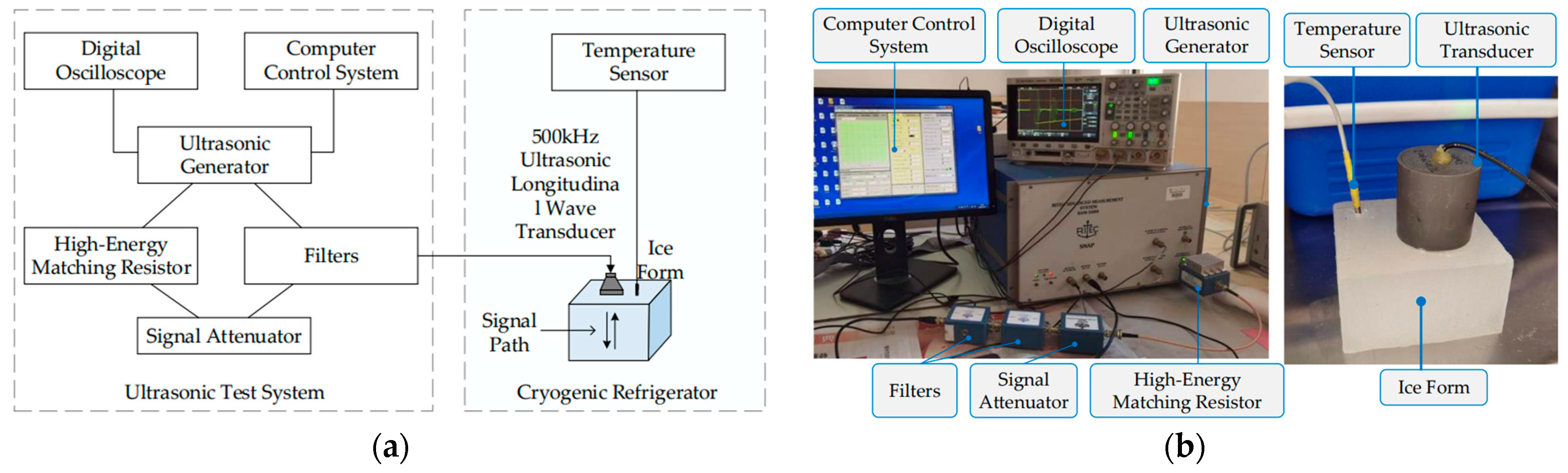
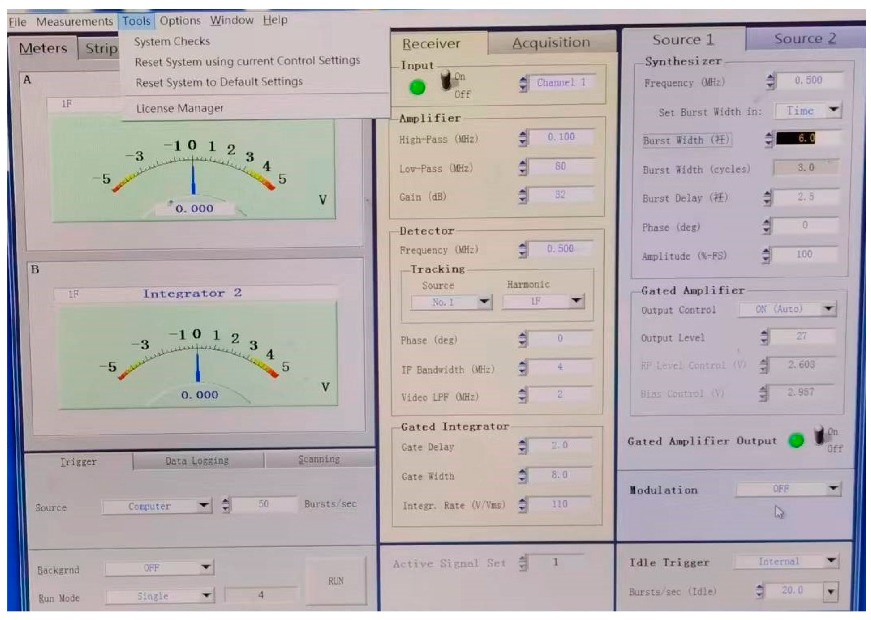
2.2. Testing Instruments

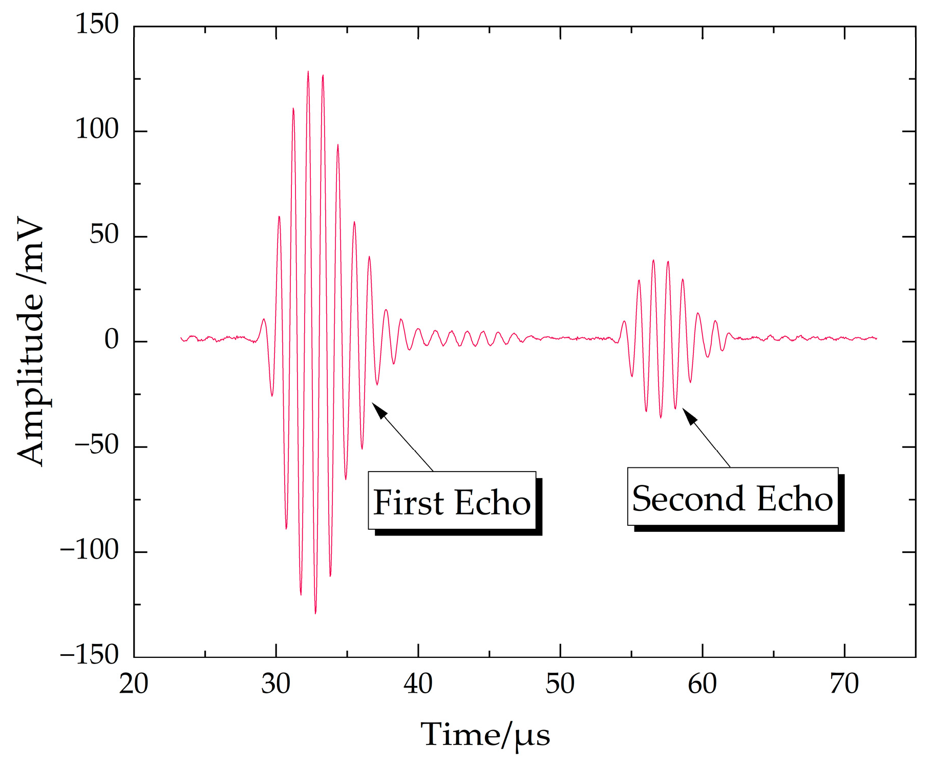
As shown in Figure 1, the test was conducted using a high-energy ultrasonic testing system to measure the speed of sound and temperature in the ice sample. The system mainly included an ultrasonic generator, a high-energy matching resistor, a signal attenuator, filters, an ultrasonic longitudinal wave transducer, a digital oscilloscope, a PT1000 platinum resistance temperature sensor, and a cryogenic freezer. The ultrasonic generator used the American RITEC RAM-5000 nonlinear high-energy ultrasonic test system (Ritec, Simi Valley, CA, USA), and a pulse signal with a centre frequency of 500 kHz was selected as the output signal. The high-energy matching resistor was used to protect the circuit and prevent the test system from being burned out; the attenuator smoothed the received ultrasonic signal curve and reduced the burr of the ultrasonic signal; a filter was used to filter out the excess noise; and the digital oscilloscope was used to observe the change in the ultrasonic signal.

2.3. Test Methods

A one-transmitter–one-receiver ultrasonic longitudinal wave transducer with a main frequency of 500 kHz was selected, and the transducer model is TR500K, which originated in Shantou, China. The propagation velocity of the ultrasound in the ice sample was measured using the pulse–echo method [19]. The thickness of the ice sample was measured using an electronic vernier calliper with an accuracy of ±0.01 mm, and an appropriate amount of a coupling agent was applied to the ultrasonic probe to fit it to the ice sample adequately and exclude the influence of air-related factors. We opened the ultrasonic test system, set the ultrasonic pulse emission frequency, the number of pulses, and other parameters, as shown in Figure 2, the pulse emission frequency is set to 0.5 MHz, the number of pulses is set to 0.5 Hz, the pulse delay is set to 2.5 µs, adjusted the pulse width and amplitude until the received ultrasonic signals were clear and smooth, observed the changes in the oscilloscope display to make it clear that the echo image is displayed several times, and then ended the adjustment. The signal changes on the oscilloscope display were observed so that it could clearly show multiple echo images, and then the adjustment was ended.

The ultrasound echo signal display is shown in Figure 3. We located the positioning ruler in the oscilloscope at the starting position of the first and second echoes, read the time between the two echoes, and obtained the propagation speed of the ultrasonic waves in the ice sample through Equation (1).

ν = 2L/∆T

(1)

where ν is the propagation velocity of the ultrasonic longitudinal wave in the ice sample, in m/s; L is the thickness of the ice sample, which is the propagation distance of the ultrasonic longitudinal wave in the ice sample, in mm; ∆T is the time between two echoes of the ultrasonic longitudinal wave, in µs.

The ice samples were stored in a low-temperature freezer throughout the test and at −35 °C for more than 24 h before the test. After the test started, we adjusted the temperature of the freezer to −30 °C, observed the change in the temperature of the ice sample through the temperature sensor, waited until the temperature of the ice sample reached −30 °C, and let it stand for 1 h to ensure the temperature of the ice sample remained constant. We coupled the ultrasonic transducer to the ice sample, observed the change in the signal on the oscilloscope, and then calculated the value of the speed of sound at this time and recorded it after it became stable. The ice sample density was measured using the mass-volume method: The length of each side of the ice sample was quickly measured and recorded using electronic vernier callipers to obtain the average length, width, and height. The volume of the ice sample was calculated, and the mass as weighed in front of the borehole was taken as the mass of the ice sample; the density of the ice sample was calculated using Equation (2).

ρ = 10⁶ × M/V

(2)

where ρ is the density of the ice sample, in kg/m³; M is the mass of the ice sample, in g; V is the volume of the ice sample, in mm³. We adjusted the temperature of the freezer to −25 °C again, monitored the temperature of the ice sample through the temperature sensor, and observed the echo signal on the oscilloscope at the same time. We recorded the time interval between the primary and secondary echoes at different temperatures during the warming process of the ice samples. After the temperature of the ice samples reached −25 °C, we left them to stand for 1 h, after which the speed of sound and the density values were measured at this temperature. We continued to increase the temperature and repeated the above tests until the sound velocity and density values were obtained for a number of temperature bands, such as −20 °C, −15 °C, −10 °C, and −5 °C. At the end of the test, the ice sample was placed in an outdoor environment to allow it to melt naturally, and the salinity of the solution obtained after the melting of the ice sample was measured using a salinometer and taken as the salinity of the ice sample. Due to the small size of the test ice samples, we did not consider the salinity in relation to the thickness change in this situation.

3. Results

A variety of sound velocity and density values for freshwater ice and saltwater ice at different temperatures were obtained from the tests, as shown in

Table 1. Density and speed of sound values at different salinities and temperatures.

Measurement Indicators	Ice Salinity (‰)	Ice Temperature (°C)
		−30	−25	−20	−15	−10	−5
Ice density (kg/m3)	0	915.5	915.1	914.3	913.4	912.9	911.9
	1.0	901.2	901.0	900.8	900.5	900.2	899.8
	1.9	904.0	903.6	903.3	903.0	902.1	901.6
	2.7	904.6	904.0	903.7	903.4	903.0	902.5
	4.5	906.7	906.3	906.0	905.7	905.5	905.2
	5.0	907.2	906.8	906.5	906.2	905.9	905.6
	5.5	908.1	907.8	907.4	907.1	906.7	906.3
	7.2	910.7	910.3	909.9	909.6	909.3	908.9
	8.5	912.9	912.5	912.1	911.7	911.4	911.9
Ice speed of sound (m/s)	0	3772.8	3765.1	3750.5	3725.5	3692.7	3659.2
	1.0	3703.8	3695.3	3681.5	3657.5	3629.8	3608.0
	1.9	3697.9	3689.6	3675.5	3651.4	3625.1	3595.3
	2.7	3687.9	3681.0	3667.9	3643.1	3623.1	3589.3
	4.5	3675.9	3668.6	3654.3	3632.4	3607.5	3574.6
	5.0	3668.9	3663.9	3650.8	3621.9	3581.3	3534.2
	5.5	3664.3	3659.8	3630.0	3593.3	3541.8
	7.2	3650.1	3644.9	3612.7	3571.6
	8.5	3627.4	3621.9	3596.4	3547.2

(only the values of sound velocity at temperatures corresponding to the measured densities are listed). During the test, with an increase in temperature, the internal structure of the high-salinity ice samples changed obviously, the attenuation of ultrasonic wave propagation in its interior increased, and the second echo was very small or even disappeared, so the speed of sound in the high-salinity ice samples at higher temperatures was not obtained.

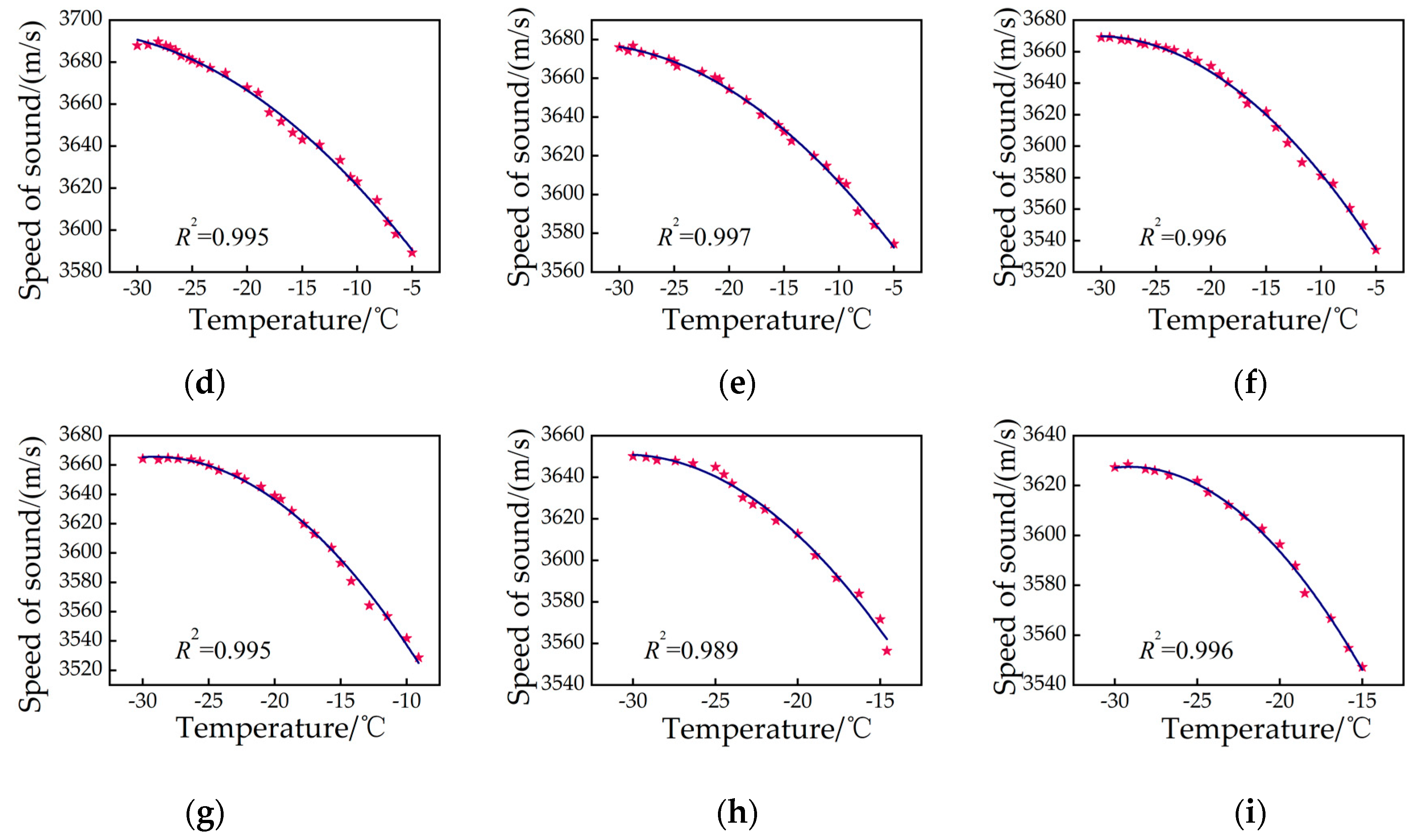
3.1. Effect of Ice Sample Temperature and Salinity on the Speed of Sound

Bogorodskii et al. [15] showed that ice, as a solid material, is capable of transmitting compression and shear waves. The compression wave speed basically varies in the range of 3200–4200 m/s, the shear wave speed varies in the range of 1450–1900 m/s, and the magnitude of the wave speed depends on the salinity and temperature of the ice. As the temperature increases, the sound velocity decreases to different degrees, and the higher the salinity of the ice sample, the lower the sound velocity. The data in Table 1 show that the measured longitudinal sound velocity of the ice samples basically varies in the range of 3500~3780 m/s. Figure 4 shows the change rule of the measured sound velocity with the salinity of the ice samples at different temperatures, and through a regression analysis, the expression of the relationship between the sound velocity and the salinity of the ice samples in the range of 0~8.5‰ salinity can be obtained, as shown in Equation (3).

ν = A₁ + B₁Si + C₁Si²

(3)

where ν is the speed of sound, in m/s; Si is the salinity of the ice sample, in ‰; and A₁, B₁, and C₁ are the fitting coefficients. The values of the fitting coefficients and the goodness of fit, R², are given in

Table 2. Equation (3) fitting coefficients and goodness of fit, R² (p < 0.05).

T (°C)	A1	B1	C1	R2
−30	3748.8	−23.17	1.19	0.845
−25	3740.1	−22.44	1.15	0.825
−20	3726.9	−22.55	0.93	0.868
−15	3701.6	−20.43	0.33	0.888
−10	3675.2	−22.14	0.36	0.752
−5	3650.1	−30.53	2.11	0.812

. As can be seen from Table 2, the regression equations have a good fit for all the temperature ranges listed, indicating that the test points are not very discrete.

As can be seen from Figure 4, as the salinity of the ice samples increases, the values of the sound velocity at the same ice temperature all decrease to different degrees, and the decreasing trend of sound velocity in the high-salinity range is slightly smaller than that in the low-salinity range. Compared with saltwater ice, freshwater ice consists only of ice crystals and a small number of gas bubbles, with a simple structure and more stable properties, so that ultrasonic waves propagate in a less attenuating manner and more rapidly in its interior. Therefore, at each temperature, the speed of sound in freshwater ice is greater than in the fitted curve.

Figure 5 shows the measured sound velocity values and quadratic fitting curves of freshwater ice and saltwater ice at different ice temperatures, as obtained in the experiments, and the goodness of fit, R², of the regression equations at each salinity is greater than 0.985. This indicates that there is a good quadratic relationship between the sound velocity and ice temperature, and the result is in line with the conclusions obtained in the study by Guo et al. [20]. In addition, it can be seen from Figure 5 that the speed of sound decreases with increasing temperature for ice samples of different salinities, a phenomenon that may be related to the decomposition of NaCl-2H₂O in the ice samples. Assur [21] and Weeks [22] studied the relationships between various salts and ion contents in sea ice with temperature and provided a sea ice phase diagram, pointing out that during the growth of ice, various salts are precipitated sequentially as the temperature decreases, and when the temperature decreases to −22.9 °C, the NaCl-2H₂O starts to precipitate. On the contrary, when the temperature of the ice sample increases, the NaCl-2H₂O stored inside the ice gradually decomposes into Na⁺, Cl⁻, H₂O. When the temperature rises to −22.9 °C, the NaCl-2H₂O is completely decomposed, and the increase in the content of Na⁺, Cl⁻, and water molecules in the ice changes the internal structure of the ice sample. The ultrasonic wave will be hindered more when it propagates inside, making the attenuation increase and the propagation speed decrease. As a result, the magnitude of the change in the speed of sound in the ice samples at each salinity level was lower than 9 m/s as the temperature increased from −30 °C to −25 °C, and the rate of decrease in the speed of sound was faster as the temperature continued to increase. According to the measured salinity of the saltwater ice, it can be divided into three salinity ranges: low salinity (1–4‰), medium salinity (4–7‰), and high salinity (more than 7‰). The test results show that, during the process of increasing the ice sample temperature from −30 °C to −5 °C, the sound velocity of freshwater ice varies within the interval of 3773~3659 m/s, the sound velocity of low-salinity saltwater ice varies within the interval of 3704~3589 m/s, the sound velocity of medium-salinity saltwater ice varies within the interval of 3676~3540 m/s, and the sound velocity of high-salinity saltwater ice varies in the temperature range of −30~−15 °C when the propagation speed varies in the interval 3651~3547 m/s.

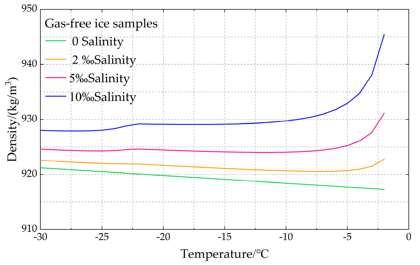
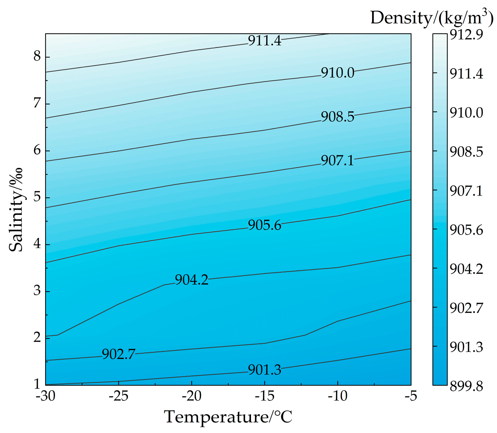
3.2. Effect of Ice Sample Temperature and Salinity on Density

Vojtkovskii et al. [23] experimentally proposed an empirical formula for the temperature dependence of the density of freshwater ice, which is 916.8 kg/m³ at 0 °C and 1 standard atmospheric pressure, and the density of ice increases by about 1.5 kg/m³ for every 10 °C drop in temperature. Cox and Weeks [24] established equations that can be used to determine the gas content of ice by measuring the ice bulk density, salinity, and temperature in the range of −2 °C to −30 °C. These relationships can be used to obtain the density of an ice sample as a function of its temperature and salinity. Timco and Frederking [25] used this equation to calculate the density of gas-free ice samples as a function of temperature for four different ice salinities (0, 2‰, 5‰, and 10‰), and the results are shown in Figure 6, where these density values represent upper bounds on ice density at the corresponding salinities and temperatures. In contrast, a certain amount of gas is present in all ice samples in the natural environment, so the measured ice sample densities are below these values.

As can be seen from Figure 6, in the temperature range of −30 to −5 °C, the densities of the gas-free ice samples of different salinities have a tendency to decrease gradually with increasing temperature (the increase in density of the high-salinity curve at −5 °C is due to the fact that the brine content within the ice becomes more abundant). The greater the salinity of the ice sample at the same ice temperature, the greater the corresponding density. And the measured density data of the ice samples with different salinities presented in Table 1 show that freshwater ice density is slightly greater than saltwater ice density when the ice temperature remains the same. This is related to the content of air bubbles in both; in the configuration of brine, there is a need to constantly stir the brine to fully dissolve the sea salt; thus, stirring caused by the disturbance of the water flow caused the brine to increase the content of air inclusions. In the low-temperature environment of the laboratory, the brine will freeze rapidly, and the air inclusions are not discharged in time and are thus frozen into the ice, forming air bubbles [12]. The greater the bubble content, the lower the density of the ice sample; meanwhile, the gas content in freshwater ice is relatively small, so in the measured data, freshwater ice density is slightly greater than the density of saltwater ice. Calculated from Table 1, the measured freshwater ice density increases linearly with a reduction in temperature, and its change rule is shown in Equation (4).

ρ = 911.3 − 0.1483T

(4)

where ρ is the density of the ice sample, in kg/m³ and T is the temperature of the ice sample, in °C. The goodness of fit (R²) = 0.99, and the density increases by about 1.483 kg/m³ for every 10 °C drop in temperature, which is basically consistent with the empirical formula for the density change in freshwater ice.

Figure 7 shows the relationship between the measured saltwater ice density with its temperature and salinity. It can be seen that when the ice temperature remains the same, the density of saltwater ice increases with increasing salinity; when the salinity remains the same, the density of saltwater ice also decreases slowly with increasing temperature. This is because with the increase in salinity of the ice sample, its brine content and bubble content will also increase, but the effect of the bubble content on the overall density is negligible, so it can be assumed that the density of the ice sample will increase with the increase in salinity. As the ice temperature continues to rise, the rate of salt decomposition accelerates, the brine content within the ice increases, the porosity increases, and the density decreases. There is a good linear functional relationship between the density of saltwater ice and its temperature and salinity. Relative to freshwater ice density, the trend of saltwater ice density with temperature is not sensitive; when the temperature decreased by 10 °C, at each salinity level, the saltwater ice showed a change in density of more than 1 kg/m³. When ice temperature remains the same, every 1‰ increase in salinity increases the density by about 1.4 kg/m³.

3.3. Exploration of the Relationship between Freshwater Ice Density and the Speed of Sound

Due to the compositions of freshwater ice and saltwater ice and the fact that their bubble contents are different, this test to measure freshwater ice against saltwater ice densities with a salinity change rule does not match; in the analysis of the relationship between the density of the ice samples and the speed of sound, there is a need to separate the two kinds of ice samples for discussion. Figure 8 shows the law of increasing density versus the speed of sound in freshwater ice, and it can be seen that there is an increasing relationship between density and the speed of sound. The lower the temperature of the ice, the greater the density of the ice, as the molecules within the ice are more tightly arranged, the ultrasonic wave propagation in its internal obstruction is smaller, and the faster the rate of vibration transmission; therefore, the greater the speed of sound is within the ice. A linear function was used to fit the law of progression for freshwater ice density versus sound velocity, and the fitting equation is shown in Equation (5).

ρ = 800.9 + 0.03ν

(5)

where ρ is the density of the ice sample, in kg/m³ and ν is the speed of sound, in m/s. The goodness of fit, R² = 0.965, indicates that there is a good linear relationship between the density and the speed of sound.

3.4. Exploration of the Relationship between Saltwater Ice Density and the Speed of Sound

This experimental study shows that both the sound velocity and density of saltwater ice show a certain regularity with changes in temperature and salinity; in order to investigate the relationship between the sound velocity and density of saltwater ice, it is necessary to analyse the relationship from the perspectives of temperature and salinity. The corresponding sound velocity and density values for the same temperature and salinity in Table 1 were plotted, as shown in Figure 9. The bars in the figure represent the relationship between the density of saltwater ice and the speed of sound at different temperatures. At the same ice temperature, there is a negative correlation between the density and the speed of sound. The greater the speed of sound, the lower the corresponding density value; the lower the temperature, the more significant the negative correlation between the density and the speed of sound. This indicates the relationship between the density of saltwater ice and the speed of sound at different salinities, and it can be observed that there is a positive correlation between density and the speed of sound for the same salinities. The greater the speed of sound, the greater the density; the lower the salinity, the more significant the positive correlation between the density and the speed of sound. Linear and quadratic curves were fitted to the pattern of change in density versus the speed of sound at each temperature and salinity, and the values of the goodness of fit, R², are shown in

Table 3. The goodness of fit, R², of the regression equation between saltwater ice density and sound velocity at different temperatures and salinities (p < 0.01).

Ice temperature (°C)		−30		−25		−20		−15		−10		−5
R2	Linear fit	0.974		0.972		0.962		0.936		0.710		0.784
	Quadratic fit	0.980		0.985		0.980		0.945		0.913		0.974
Ice salinity (‰)		1	1.9		2.7		4.5	5	5.5		7.2		8.5
R2	Linear fit	0.990	0.988		0.925		0.931	0.908	0.931		0.903		0.863
	Quadratic fit	0.992	0.989		0.949		0.974	0.966	0.964		0.952		0.974

.

The data in Table 3 show that the linear and quadratic relationships between the density of saltwater ice and the speed of sound are well fitted, and the R² values do not differ much at the four temperatures of −30 °C, −25 °C, −20 °C, and −15 °C, while the quadratic functions of the density and the speed of sound at the temperatures of −10 °C and −5 °C are fitted significantly better than the linear functions, and the same phenomenon is also observed in the range of salinity scales. To ensure a good correlation between density and the speed of sound, a quadratic function is used in this paper to characterise the correlation between the speed of sound and the density of saltwater ice at different temperatures and salinities.

4. Development and Evaluation of Ice Density Prediction Model

In order to realise the possibility of inverting ice density through the acoustic properties of ice, this paper obtains the pattern of changes in density with sound speed, temperature, and salinity in artificially frozen ice samples with the aim of using the latter three variables to parameterise the former and ultimately to establish a predictive model for ice density. According to the above analysis, it can be seen that the internal group structures of freshwater ice and saltwater ice are different, the ice temperature remains the same, the speed of sound in the freshwater ice is obviously greater than the saltwater ice, and the densities of freshwater ice and saltwater ice do not match with the change rule of salinity. In order to avoid introducing large errors, the following functions are proposed to estimate the freshwater ice and saltwater ice densities separately using the measured data in Table 1:

$$\rho =\left\{\begin{array}{cc}{\mathrm{k}}_{\mathrm{a}1}+{\mathrm{k}}_{\mathrm{a}2}T+{\mathrm{k}}_{\mathrm{a}3}\nu & Si=0\\ {\mathrm{k}}_{\mathrm{b}1}+{\mathrm{k}}_{\mathrm{b}2}T+{\mathrm{k}}_{\mathrm{b}3}\nu +{\mathrm{k}}_{\mathrm{b}4}{\nu }^2+{\mathrm{k}}_{\mathrm{b}5}Si& Si>0\end{array}\right.$$

(6)

where k_a1, k_a2, k_a3, k_b1, k_b2, k_b3, k_b4, and k_b5 are the correlation coefficients obtained using a least squares regression, as shown in

Table 4. Equation (6) least squares regression coefficients and model evaluation indicators.

Parametric	ka1 (kb1)	ka2 (kb2)	ka3 (kb3)	kb4	kb5	R2	p	RMSE	MAE	MAPE
Si = 0	880.47	−0.1092	0.0084			0.993	<0.001	0.337	0.257	0.03%
Si > 0	928.9	−0.065	−0.019	2.81 × 10−6	1.44

; T is the temperature of the ice sample, in °C; Si is the salinity of the ice sample, in ‰; ν is the propagation velocity, in m/s; and ρ is the density of the ice sample, in kg/m³.

As can be seen from Table 4, the R² of the prediction model is greater than 0.95, and the RMSE, MAE, and MAPE are 0.337 kg/m³, 0.257 kg/m³, and 0.03%, respectively, which indicates that the error between the model prediction value and the measured value is small, and the degree of fit is high. The confidence (two-sided) statistic p is lower than 0.001; the model regression effect is significant; the prediction accuracy is good; and the prediction of ice density can be achieved with some statistical significance.

The results of the residuals between the measured and predicted values of the ice density prediction model at different temperatures and salinities are shown in Figure 10, and the white part is due to the fact that the measured values of the sound velocity of the ice samples are unknown at those temperatures and salinities, and therefore the predicted values of their densities were not obtained. The residuals of the prediction model were calculated to be in the range of −0.674 to 0.855 kg/m³, and, as can be seen from Figure 10, the residual values did not show a certain distribution pattern or trend of change with the density of the ice samples, which indicates that these residuals are better left independent. At temperatures from −20 to −5 °C, the model prediction accuracy is better, with all residual values lower than 0.4 kg/m³, while at temperatures from −30 to −25 °C, the prediction accuracy is relatively poor. In terms of salinity, the prediction accuracy for the density of freshwater ice is overall better than for that of saltwater ice, with a maximum error of no more than 0.2 kg/m³; for saltwater ice density, the model has the highest prediction accuracy in the range of medium salinity (4–7‰), followed by the range of high salinity (more than 7‰), and the prediction accuracy in the range of low salinity (1–4‰) is poor. Analysing the density data in Table 1, it can be seen that when the ice sample temperature is at −30~−25 °C and the salinity is at 1~4‰, the linear correlation between the density of the ice sample and the ice temperature and salinity is weak, so the prediction accuracy of the model is relatively poor. At the same time, the large salinity intervals between the ice samples measured in the low-salinity range have an impact on the prediction accuracy of the model, which can be improved by increasing the number of test ice samples in this salinity range.

Figure 11 shows a four-dimensional statistical plot of the density of brackish water ice in the prediction model, where the grid surface represents the relationships between the speed of sound and temperature and salinity. The colour mapping on the surface depicts the relationship between the salty water ice density with the speed of sound at different temperatures and salinities. The point map represents the measured sound velocity values, and the colour mapping on the point map represents the measured density values.

5. Conclusions

In this paper, the acoustic and physical properties of artificially frozen ice samples with salinities ranging from 0 to 8.5‰ were tested using a nonlinear high-energy ultrasonic testing system. The following conclusions were drawn from the analysis of the measured ice sample density, sound velocity, temperature, and salinity data:

(1)

In the temperature range of −30~−5 °C, there is a good quadratic relationship between the speed of sound in the ice samples and both temperature and salinity. When the salinity remains the same, the speed of sound in the ice samples decreases gradually with an increase in temperature. The change in the speed of sound is not obvious when the temperature rises from −30 °C to −25 °C, and the speed of sound decreases faster as the temperature continues to rise. When the ice temperature remains the same, with increasing salinity of the ice samples, the value of the speed of sound has different degrees of reduction, and the rate of change in the speed of sound in the high-salinity range is lower than that in the low-salinity range. Compared with saltwater ice, freshwater ice has a simpler structure, and when the ice temperature remains the same, the speed of sound in freshwater ice is significantly greater than that in saltwater ice.

(2)

There is a good linear relationship between the density of ice samples and both temperature and salinity in the temperature range of −30 to −5 °C. With an increase in temperature, the density of the ice samples with different salinities showed a tendency to decrease. The density of freshwater ice was slightly greater than that of saltwater ice, and its value varied within the interval of 911.9~915.5 kg/m³. When the ice temperature remains the same, the density of saltwater ice increases with an increase in salinity, and its value varies in the range of 899.8–912.9 kg/m³; compared with the temperature, the trend of saltwater ice density with a change in salinity is more sensitive.

(3)

There is a linearly increasing relationship between the density of freshwater ice and the speed of sound; the greater the density, the greater the speed of sound. The relationship between the density of saltwater ice and the speed of sound shows different regularities, depending on the ice temperature and salinity. For the same ice temperature, the density of saltwater ice decreases gradually with an increasing speed of sound; for the same salinity, the density of saltwater ice increases with an increasing speed of sound. Using the rules of change in ice density with temperature, salinity, and sound speed obtained from the test, the prediction model of ice density on temperature, salinity, and sound speed was established, and the model prediction accuracy is good, which can satisfy the demand for the prediction of ice density.

In the context of global warming, ice conditions on water are changing, especially in the rapid melting of sea ice, leading to corresponding changes in its physical properties. The ice density prediction model proposed in this paper can provide a new idea for sea ice density monitoring. Temperature, salinity, and sound speed monitoring devices can be integrated into sea ice buoys for real-time online monitoring of the physical and acoustic properties of sea ice, thus realising the online monitoring of spatial and temporal changes in sea ice density.

References

1. Wang, J.; Li, Z.; Cheng, T.; Sui, J. Time-dependent local scour around bridge piers under ice cover-an experimental study. J. Hydraul. Eng. 2021, 52, 1174–1182. [Google Scholar]
2. Ding, F.; Mao, Z. Ice cover growth-decay proces of pond in cold region. J. Hydraul. Eng. 2021, 52, 349–358. [Google Scholar]
3. Wang, E.; Hu, S.; Han, H.; Liu, C. Research on ice concentration in Heilong River based on the UAV low-altitude remote sensing and OTSU algorithm. J. Hydraul. Eng. 2022, 53, 68–77. [Google Scholar]
4. Li, B.; Pang, X.; Ji, Q. Analyses of arctic sea ice density variation and its impact on sea ice thickness retrieval. Chin. J. Polar Res. 2019, 31, 258–266. [Google Scholar]
5. Li, Z.; Zhou, Q.; Wang, E.; Jia, Q. Experimental study on the loading mode effects on the ice uniaxial compressive strength. J. Hydraul. Eng. 2013, 44, 1037–1043. [Google Scholar]
6. Alexandrov, V.; Sandven, S.; Wahlin, J.; Johannessen, O.M. The relation between sea ice thickness and freeboard in the Arctic. Cryosphere 2010, 4, 373–380. [Google Scholar] [CrossRef]
7. Li, Z.; Nicolaus, M.; Toyota, T.; Haas, C. Analysis on the crystals of sea ice cores derived from weddell sea, Antarctica. Chin. J. Polar Res. 2009, 21, 177–185. [Google Scholar]
8. Lin, Y.; Xu, Y.; Gu, W.; Bu, D.; Yuan, S. Distribution of sea ice density and air porosity along the coast of the Bohai Sea. Resour. Sci. 2010, 32, 412–416. [Google Scholar]
9. Sallila, H.; Farrell, S.L.; McCurry, J.; Rinne, E. Assessment of contemporary satellite sea ice thickness products for Arctic sea ice. Cryosphere 2019, 13, 1187–1213. [Google Scholar] [CrossRef]
10. Wang, Q.; Li, Z.; Lei, R.; Lu, P.; Han, H. Estimation of the uniaxial compressive strength of Arctic sea ice during melt season. Cold Reg. Sci. Technol. 2018, 151, 9–18. [Google Scholar] [CrossRef]
11. Ji, Q.; Li, B.; Pang, X.; Zhao, X.; Lei, R. Arctic sea ice density observation and its impact on sea ice thickness retrieval from CryoSat-2. Cold Reg. Sci. Technol. 2021, 181, 103177. [Google Scholar] [CrossRef]
12. Zhang, Y.; Li, Z.; Li, C.; Zhang, B.; Deng, Y. Microstructure characteristics of river ice in Inner Mongolia section of the Yellow River and its influencing factors. J. Hydraul. Eng. 2021, 52, 1418–1429. [Google Scholar]
13. Zuo, G.; Dou, Y.; Chang, X.; Chen, Y.; Ma, C. Design and performance analysis of a Multilayer Sea Ice temperature sensor used in polar region. Sensors 2018, 18, 4467. [Google Scholar] [CrossRef] [PubMed]
14. Langleben, M.P. Attenuation of sound in sea ice, 10–500 kHz. J. Glaciol. 1969, 8, 399–406. [Google Scholar] [CrossRef]
15. Bogorodskii, V.V.; Gavrilo, V.P.; Gusev, A.V.; Nikitin, V.A. Measurements of speed of ultrasonic-waves in Bering sea ice. Sov. Phys. Acoust. 1975, 21, 286–287. [Google Scholar]
16. Chang, X.; Liu, W.; Zuo, G.; Dou, Y.; Li, Y. Research on ultrasonic-based investigation of mechanical properties of ice. Acta Oceanol. Sin. 2021, 40, 97–105. [Google Scholar] [CrossRef]
17. Feng, C.; Liu, Q.; Zhang, J. Porosity based ice sound velocity model and its empirical formula. Tech. Acoust. 2017, 36, 509–515. [Google Scholar]
18. Zhang, M.; Shao, C. The materialization of sea ice. Mar. Sci. Bull. 1981, 5, 36–43. [Google Scholar]
19. Chen, J.; Gong, G.; Gao, W.; Zhou, J. Comprehensive experiment of ultrasonic testing. Phys. Exp. 2016, 36, 24–27, 34. [Google Scholar]
20. Guo, Y.; Li, G.; Jia, C.; Chang, T.; Cui, H.; Markov, A. Study of ultrasonic test in the measurements of mechanical properties of ice. Chin. J. Polar Res. 2016, 28, 152–157. [Google Scholar]
21. Assur, A. Composition of Sea Ice and Its Tensile Strength; US Army Snow, Ice and Permafrost Research Establishment: Wilmette, IL, USA, 1960; pp. 12–18. [Google Scholar]
22. Weeks, W.F.; Ackley, S.F. The Growth, Structure, and Properties of Sea Ice. In The Geophysics of Sea Ice; Springer: Boston, MA, USA, 1986; pp. 105–116. [Google Scholar]
23. Voitkovskii, K.F. The Mechanical Properties of Ice; American Meteorological Society: Boston, MA, USA, 1962; pp. 21–57. [Google Scholar]
24. Cox, G.F.; Weeks, W.F. Equations for determining the gas and brine volumes in sea-ice samples. J. Glaciol. 1983, 29, 306–316. [Google Scholar] [CrossRef]
25. Timco, G.W.; Frederking, R.M. A review of sea ice density. Cold Reg. Sci. Technol. 1996, 24, 1–6. [Google Scholar] [CrossRef]
Figure 1. Instrument connection diagram and test platform. (a) Instrument connection diagram. (b) Test platform.
Water 15 04065 g001
Figure 2. Parameter control interface.
Water 15 04065 g002
Figure 3. Ultrasound echo signal.
Water 15 04065 g003
Figure 4. Relationship between the speed of sound and the salinity of ice samples at different temperatures.
Water 15 04065 g004
Figure 5. Relationship between the speed of sound and temperature in ice samples at different salinities: (a) freshwater ice, (b) 1.0‰ saltwater ice, (c) 1.9‰ saltwater ice, (d) 2.7‰ saltwater ice, (e) 4.5‰ saltwater ice, (f) 5.0‰ saltwater ice, (g) 5.5‰ saltwater ice, (h) 7.2‰ saltwater ice, and (i) 8.5‰ saltwater ice.
Water 15 04065 g005aWater 15 04065 g005b
Figure 6. Relationship between density and temperature for four different salinities of gas-free ice samples.
Water 15 04065 g006
Figure 7. Relationship between measured saltwater ice density and its temperature and salinity.
Water 15 04065 g007
Figure 8. The law of density–sound rapid change in freshwater ice.
Water 15 04065 g008
Figure 9. Relationship between saltwater ice density and sound velocity at different temperatures and salinities.
Water 15 04065 g009
Figure 10. Ice density prediction model residual results.
Water 15 04065 g010
Figure 11. Saltwater ice density prediction modelling statistics.
Water 15 04065 g011