
A New Method for Estimating Groundwater Changes Based on Optimized Deep Learning Models—A Case Study of Baiquan Spring Domain in China
Abstract
:1. Introduction
2. Materials and Methods
2.1. Data
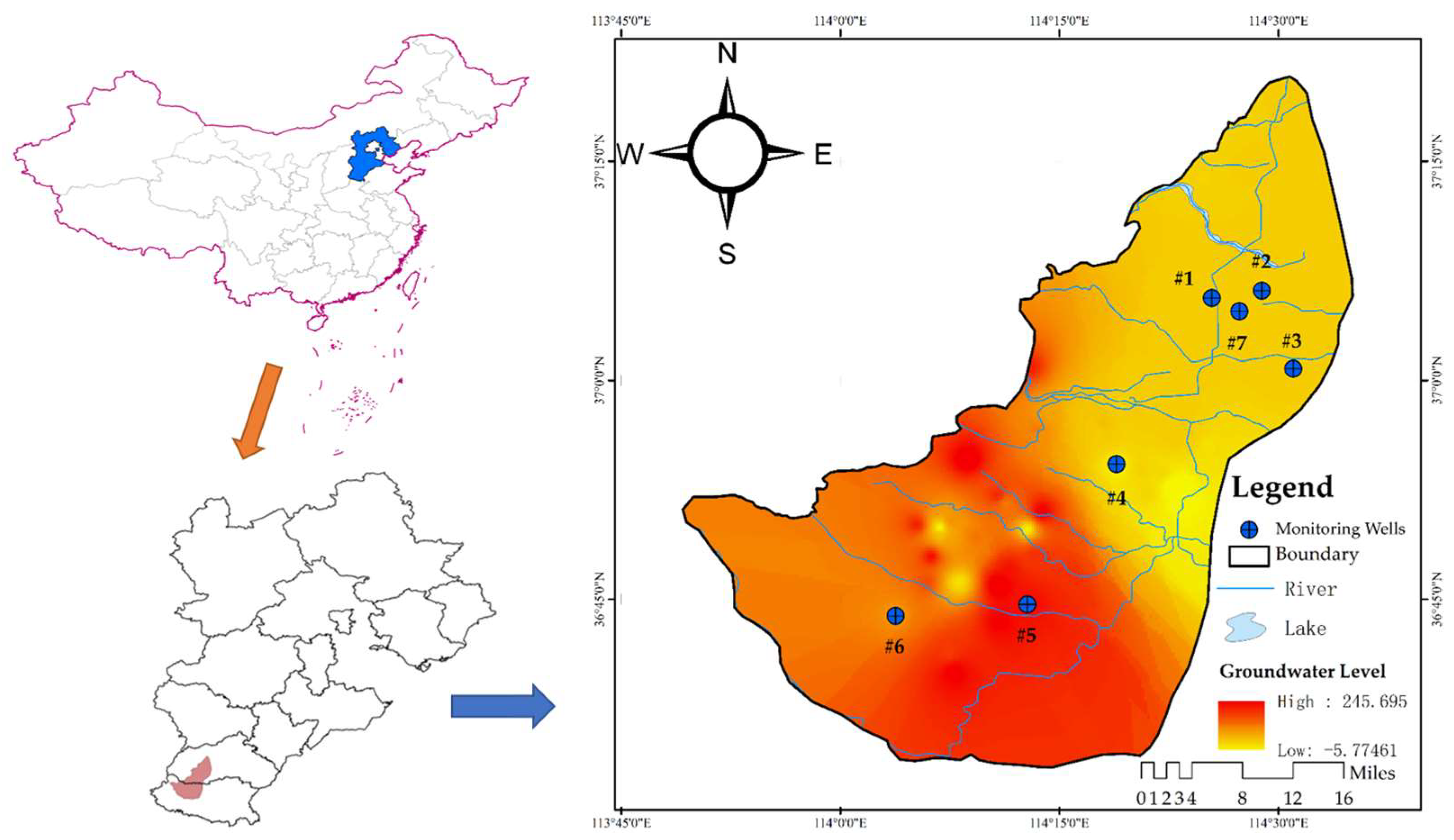
2.1.1. Dataset Description
2.1.2. Empirical Observation
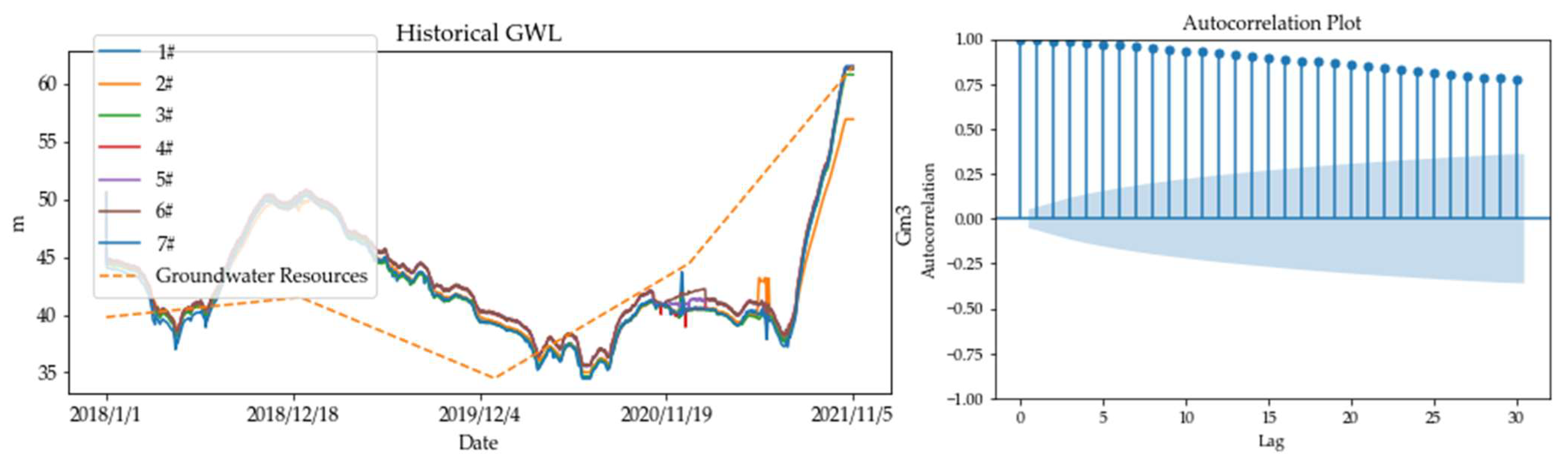
- Microlevel: Historical GWL Observation
- 2.
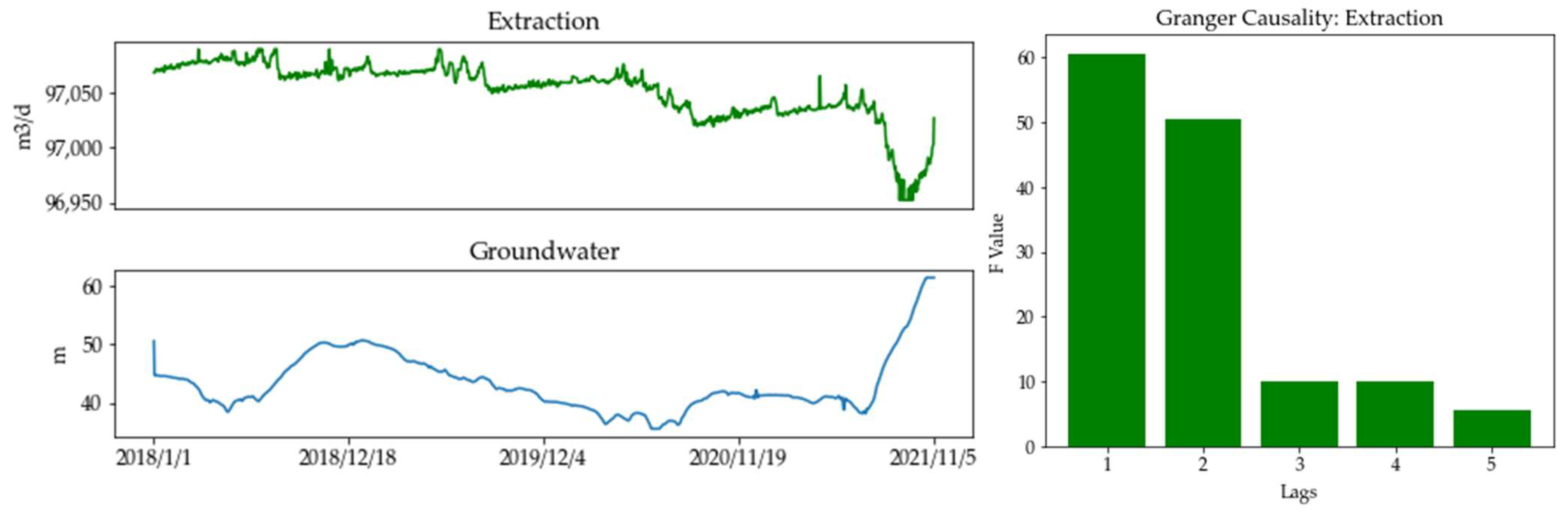
- Mesolevel: Precipitation and Extraction Observation
- 3.
- Macrolevel: Policy Observation
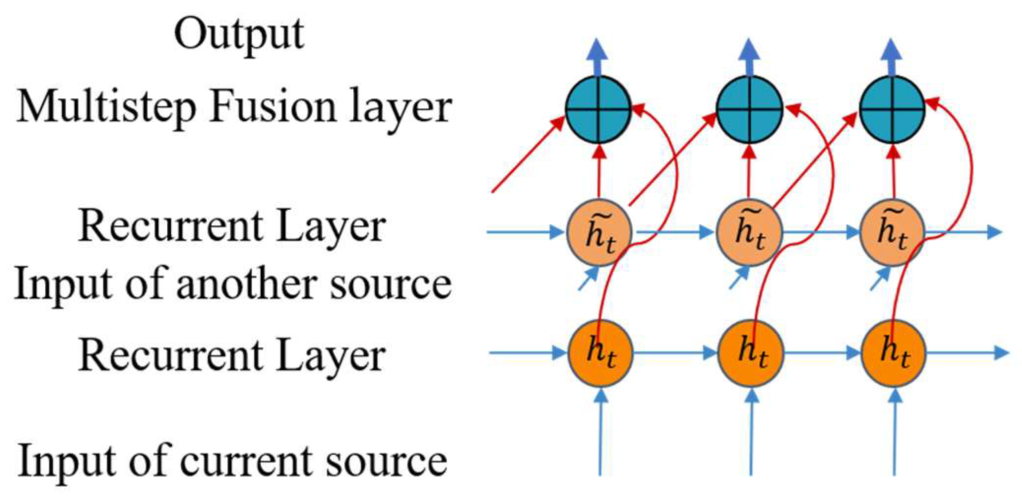
2.2. Model
2.3. Model Evaluation
3. Results
4. Discussion
5. Conclusions
Author Contributions
Funding
Data Availability Statement
Conflicts of Interest
References
- Liu, J.T.; Gao, Z.J.; Wang, M.; Li, Y.Z.; Ma, Y.Y.; Shi, M.J.; Zhang, H.Y. Study on the dynamic characteristics of groundwater in the valley plain of Lhasa City. Environ. Earth Sci. 2018, 77, 646. [Google Scholar] [CrossRef]
- Yang, J.; Yu, Z.; Yi, P.; Aldahan, A. Assessment of groundwater quality and Rn-222 distribution in the Xuzhou region, China. Environ. Monit. Assess. 2018, 190, 1–12. [Google Scholar] [CrossRef]
- Lo, W.; Purnomo, S.N.; Sarah, D.; Aghnia, S.; Hardini, P. Groundwater Modelling in Urban Development to Achieve Sustainability of Groundwater Resources: A Case Study of Semarang City, Indonesia. Water 2021, 13, 1395. [Google Scholar] [CrossRef]
- Sahoo, S.; Jha, M.K.; Kumar, N.; Chowdary, V.M. Evaluation of GIS-based multicriteria decision analysis and probabilistic modeling for exploring groundwater prospects. Environ. Earth Sci. 2015, 74, 2223–2246. [Google Scholar] [CrossRef]
- Yousefi, H.; Zahedi, S.; Niksokhan, M.H.; Momeni, M. Ten-year prediction of groundwater level in Karaj plain (Iran) using MODFLOW2005-NWT in MATLAB. Environ. Earth Sci. 2019, 78, 14. [Google Scholar] [CrossRef]
- Yadav, B.; Gupta, P.K.; Patidar, N.; Himanshu, S.K. Ensemble modelling framework for groundwater level prediction in urban areas of India. Sci. Total Environ. 2020, 712, 135539. [Google Scholar] [CrossRef] [PubMed]
- Barzegar, R.; Fijani, E.; Moghaddam, A.A.; Tziritis, E. Forecasting of groundwater level fluctuations using ensemble hybrid multi-wavelet neural network-based models. Sci. Total Environ. 2017, 599, 20–31. [Google Scholar] [CrossRef]
- Osman, A.I.A.; Ahmed, A.N.; Chow, M.F.; Huang, Y.F.; El-Shafie, A. Extreme gradient boosting (Xgboost) model to predict the groundwater levels in Selangor Malaysia. Ain Shams Eng. J. 2021, 12, 1545–1556. [Google Scholar] [CrossRef]
- Alizamir, M.; Kim, S.; Kisi, O.; Zounemat-Kermani, M. A comparative study of several machine learning based non-linear regression methods in estimating solar radiation: Case studies of the USA and Turkey regions. Energy 2020, 197, 117239. [Google Scholar] [CrossRef]
- Lai, Z.-H.; Kiang, J.-F.; IEEE. Water-Table Detection in a Hyper-Arid Region. In Proceedings of the USNC-URSI Radio Science Meeting/IEEE International Symposium on Antennas and Propagation (AP-S), Atlanta, GA, USA, 7–12 July 2019; pp. 107–108. [Google Scholar]
- Huang, M.; Tian, Y. Prediction of Groundwater Level for Sustainable Water Management in an Arid Basin Using Data-driven Models. In Proceedings of the 2015 International Conference on Sustainable Energy and Environmental Engineering (IEEE), Bangkok, Thailand, 25–26 October 2015; pp. 134–137. [Google Scholar]
- Lu, Y.; Ke, C.-Q.; Zhou, X.; Wang, M.; Lin, H.; Chen, D.; Jiang, H. Monitoring land deformation in Changzhou city (China) with multi-band InSAR data sets from 2006 to 2012. Int. J. Remote Sens. 2017, 39, 1151–1174. [Google Scholar] [CrossRef]
- Khaki, M.; Yusoff, I.; Islami, N.; Hussin, N.H. Artificial Neural Network Technique for Modeling of Groundwater Level in Langat Basin, Malaysia. Sains Malays 2016, 45, 19–28. [Google Scholar]
- Ahmadi, A.; Olyaei, M.; Heydari, Z.; Emami, M.; Zeynolabedin, A.; Ghomlaghi, A.; Daccache, A.; Fogg, G.E.; Sadegh, M. Groundwater Level Modeling with Machine Learning: A Systematic Review and Meta-Analysis. Water 2022, 14, 949. [Google Scholar] [CrossRef]
- Pham, Q.B.; Kumar, M.; Di Nunno, F.; Elbeltagi, A.; Granata, F.; Islam, A.R.M.T.; Talukdar, S.; Nguyen, X.C.; Ahmed, A.N.; Anh, D.T. Groundwater Level Prediction Using Machine Learning Algorithms in a Drought-Prone Area. Neural Comput. Appl. 2022, 34, 10751–10773. [Google Scholar] [CrossRef]
- Samani, S.; Vadiati, M.; Nejatijahromi, Z.; Etebari, B.; Kisi, O. Groundwater Level Response Identification by Hybrid Wavelet–Machine Learning Conjunction Models Using Meteorological Data. Environ. Sci. Pollut. Res. 2022, 30, 22863–22884. [Google Scholar] [CrossRef] [PubMed]
- Cai, H.; Liu, S.; Shi, H.; Zhou, Z.; Jiang, S.; Babovic, V. Toward Improved Lumped Groundwater Level Predictions at Catchment Scale: Mutual Integration of Water Balance Mechanism and Deep Learning Method. J. Hydrol. 2022, 613, 128495. [Google Scholar] [CrossRef]
- Shamsuddin, M.K.N.; Kusin, F.M.; Sulaiman, W.N.A.; Ramli, M.F.; Baharuddin, M.F.T.; Adnan, M.S. Forecasting of Groundwater Level using Artificial Neural Network by incorporating river recharge and river bank infiltration. In Proceedings of the International Symposium on Civil and Environmental Engineering (ISCEE), Melaka, Malaysia, 5–6 December 2016. [Google Scholar] [CrossRef]
- Chitsazan, M.; Rahmani, G.; Neyamadpour, A. Forecasting groundwater level by artificial neural networks as an alternative approach to groundwater modeling. J. Geol. Soc. India 2015, 85, 98–106. [Google Scholar] [CrossRef]
- Natarajan, N.; Sudheer, C. Groundwater level forecasting using soft computing techniques. Neural Comput. Appl. 2019, 32, 7691–7708. [Google Scholar] [CrossRef]
- Kayhomayoon, Z.; Babaeian, F.; Milan, S.G.; Azar, N.A.; Berndtsson, R. A Combination of Metaheuristic Optimization Algorithms and Machine Learning Methods Improves the Prediction of Groundwater Level. Water 2022, 14, 751. [Google Scholar] [CrossRef]
- Di Nunno, F.; Granata, F. Groundwater level prediction in Apulia region (Southern Italy) using NARX neural network. Environ. Res. 2020, 190, 110062. [Google Scholar] [CrossRef]
- Takeuchi, D.; Yatabe, K.; Koizumi, Y.; Oikawa, Y.; Harada, N.; IEEE. Real-Time Speech Enhancement Using Equilibriated Rnn. In Proceedings of the IEEE International Conference on Acoustics, Speech, and Signal Processing, Barcelona, Spain, 4–8 May 2020; pp. 851–855. [Google Scholar]
- Baek, Y.; Kim, H.Y. ModAugNet: A new forecasting framework for stock market index value with an overfitting prevention LSTM module and a prediction LSTM module. Expert Syst. Appl. 2018, 113, 457–480. [Google Scholar] [CrossRef]
- Bryngelson, S.H.; Charalampopoulos, A.; Sapsis, T.P.; Colonius, T. A Gaussian moment method and its augmentation via LSTM recurrent neural networks for the statistics of cavitating bubble populations. Int. J. Multiph. Flow 2020, 127, 103262. [Google Scholar] [CrossRef]
- Massaoudi, M.; Abu-Rub, H.; Refaat, S.S.; Chihi, I.; Oueslati, F.S. Deep Learning in Smart Grid Technology: A Review of Recent Advancements and Future Prospects. IEEE Access 2021, 9, 54558–54578. [Google Scholar] [CrossRef]
- Elsayed, N.; Maida, A.S.; Bayoumi, M.; IEEE. Gated Recurrent Neural Networks Empirical Utilization for Time Series Classification. In Proceedings of the IEEE International Conference on Cybermat/12th IEEE International Conference on Cyber, Physical and Social Comp (CPSCom)/15th IEEE International Conference on Green Computing and Communications (GreenCom)/12th IEEE Int Conf on Internet of Things (iThings)/5th IEEE Int Conf on Smart Data, Atlanta, GA, USA, 14–17 July 2019; pp. 1207–1210. [Google Scholar]
- Ao, C.; Zeng, W.; Wu, L.; Qian, L.; Srivastava, A.K.; Gaiser, T. Time-delayed machine learning models for estimating groundwater depth in the Hetao Irrigation District, China. Agric. Water Manag. 2021, 255. [Google Scholar] [CrossRef]
- Baek, J.M.; Shibuya, S.; Furumiya, M.; Saito, M.; Lohani, T.N.; Hur, J.S. Case study on evaluating the groundwater seepage flow by using a 3D ground model prepared from soil borehole and GIS data. In Proceedings of the Computer Methods and Recent Advances in Geomechanics, Kyoto, Japan, 22–25 September 2014; pp. 841–845. [Google Scholar]
- Li, P.; Tian, R.; Xue, C.; Wu, J. Progress, opportunities, and key fields for groundwater quality research under the impacts of human activities in China with a special focus on western China. Environ. Sci. Pollut. Res. 2017, 24, 13224–13234. [Google Scholar] [CrossRef] [PubMed]
- Hu, W.; Yang, Y.; Wang, J.; Huang, X.; Cheng, Z. Understanding Electricity-Theft Behavior via Multi-Source Data. In Proceedings of the Web Conference 2020, Taipei, Taiwan, 20–24 April 2020; pp. 2264–2274. [Google Scholar]
- Wang, R.; Li, X.; Wei, A. Hydrogeochemical characteristics and gradual changes of groundwater in the Baiquan karst spring region, northern China. Carbonates Evaporites 2022, 37, 47. [Google Scholar] [CrossRef]
- Maziarz, M. A review of the Granger-causality fallacy. J. Philos. Econ. 2015, VIII, 10676. [Google Scholar] [CrossRef]
- Cai, X.; Sun, H.; Zhang, Q.; Huang, Y. A Grid Weighted Sum Pareto Local Search for Combinatorial Multi and Many-Objective Optimization. IEEE Trans. Cybern. 2019, 49, 3586–3598. [Google Scholar] [CrossRef]
- Gao, M.; Yang, F.; Wei, H.; Liu, X. Automatic Monitoring of Maize Seedling Growth Using Unmanned Aerial Vehicle-Based RGB Imagery. Remote Sens. 2023, 15, 3671. [Google Scholar] [CrossRef]
- He, S.; Wu, J.; Wang, D.; He, X. Predictive Modeling of Groundwater Nitrate Pollution and Evaluating Its Main Impact Factors Using Random Forest. Chemosphere 2021, 290, 133388. [Google Scholar] [CrossRef]
- Gao, M.; Yang, F.; Wei, H.; Liu, X. Individual Maize Location and Height Estimation in Field from UAV-Borne LiDAR and RGB Images. Remote Sens. 2022, 14, 2292. [Google Scholar] [CrossRef]
- Chai, T.; Draxler, R.R. Root mean square error (RMSE) or mean absolute error (MAE)?—Arguments against avoiding RMSE in the literature. Geosci. Model Dev. 2014, 7, 1247–1250. [Google Scholar] [CrossRef]
- Iqbal, N.; Khan, A.-N.; Rizwan, A.; Ahmad, R.; Kim, B.W.; Kim, K.; Kim, D.-H. Groundwater Level Prediction Model Using Correlation and Difference Mechanisms Based on Boreholes Data for Sustainable Hydraulic Resource Management. IEEE Access 2021, 9, 96092–96113. [Google Scholar] [CrossRef]
- Naghibi, S.A.; Ahmadi, K.; Daneshi, A. Application of Support Vector Machine, Random Forest, and Genetic Algorithm Optimized Random Forest Models in Groundwater Potential Mapping. Water Resour. Manag. 2017, 31, 2761–2775. [Google Scholar] [CrossRef]
- Lallahem, S.; Mania, J.; Hani, A.; Najjar, Y. On the use of neural networks to evaluate groundwater levels in fractured media. J. Hydrol. 2005, 307, 92–111. [Google Scholar] [CrossRef]
- Provincial Water Resources Department Held a Pilot Conference on Groundwater Recharge of River and Lake in Hebei Province. Available online: http://slt.hebei.gov.cn/a/2018/09/12/2018091236969.html (accessed on 12 September 2018).
- The Total Volume of Water Replenished by the Hebei Groundwater Recharge Pilot Project Has Surpassed 100 Million Cubic Meters. Available online: http://slt.hebei.gov.cn/a/2018/10/16/2018101637396.html (accessed on 16 October 2018).
- The Provincial Department of Water Resources Convenes a Provincial Water Administration Work Conference. Available online: http://slt.hebei.gov.cn/a/2021/05/17/216A7F2DA703410299D478D8846DF438.html (accessed on 17 May 2021).
- Mohanty, S.; Jha, M.K.; Raul, S.K.; Panda, R.K.; Sudheer, K.P. Using Artificial Neural Network Approach for Simultaneous Forecasting of Weekly Groundwater Levels at Multiple Sites. Water Resour. Manag. 2015, 29, 5521–5532. [Google Scholar] [CrossRef]
- Rajaee, T.; Ebrahimi, H.; Nourani, V. A review of the artificial intelligence methods in groundwater level modeling. J. Hydrol. 2019, 572, 336–351. [Google Scholar] [CrossRef]
- Mukherjee, A.; Ramachandran, P. Prediction of GWL with the help of GRACE TWS for unevenly spaced time series data in India: Analysis of comparative performances of SVR, ANN and LRM. J. Hydrol. 2018, 558, 647–658. [Google Scholar] [CrossRef]
- Liu, F.; Zhang, Z.; Zhou, R. Automatic modulation recognition based on CNN and GRU. Tsinghua Sci. Technol. 2022, 27, 422–431. [Google Scholar] [CrossRef]


| Methods | NSE | RMSE | MAE | R2 | ||||
|---|---|---|---|---|---|---|---|---|
| Train | Test | Train | Test | Train | Test | Train | Test | |
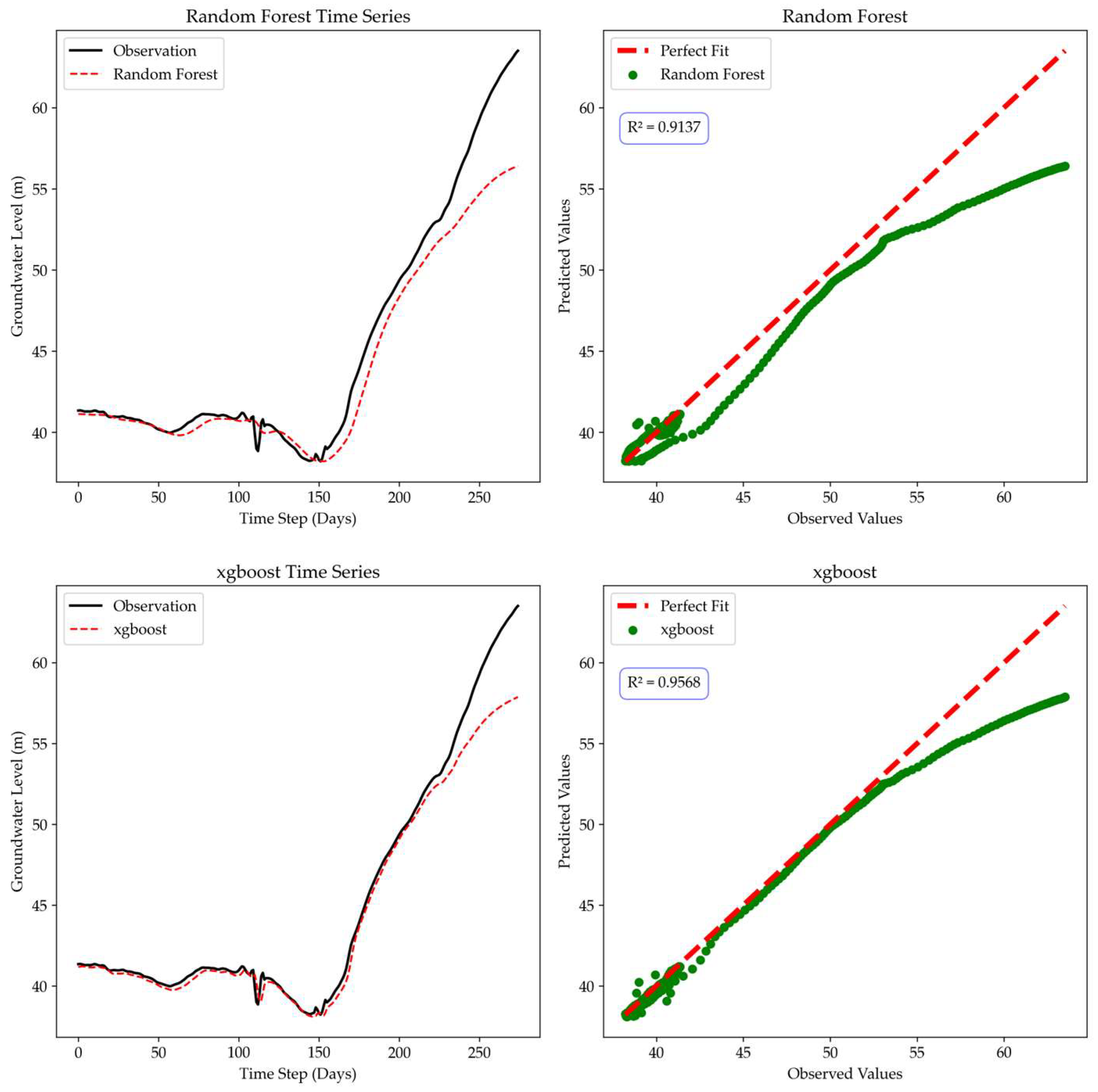
| Random Forest | 0.9891 | 0.9160 | 0.0292 | 0.1192 | 0.3376 | 1.3097 | 0.9890 | 0.9137 |
| XGBoost | 0.9977 | 0.9573 | 0.0130 | 0.0775 | 0.1494 | 0.8094 | 0.9977 | 0.9568 |
| SVM | 0.9987 | 0.9560 | 0.0100 | 0.0801 | 0.1068 | 0.7737 | 0.9987 | 0.9557 |
| HGP | 0.9994 | 0.9933 | 0.0069 | 0.0259 | 0.0838 | 0.3758 | 0.9994 | 0.9933 |
| Method | NSE | RMSE | MAE | R2 | ||||
|---|---|---|---|---|---|---|---|---|
| Train | Test | Train | Test | Train | Test | Train | Test | |
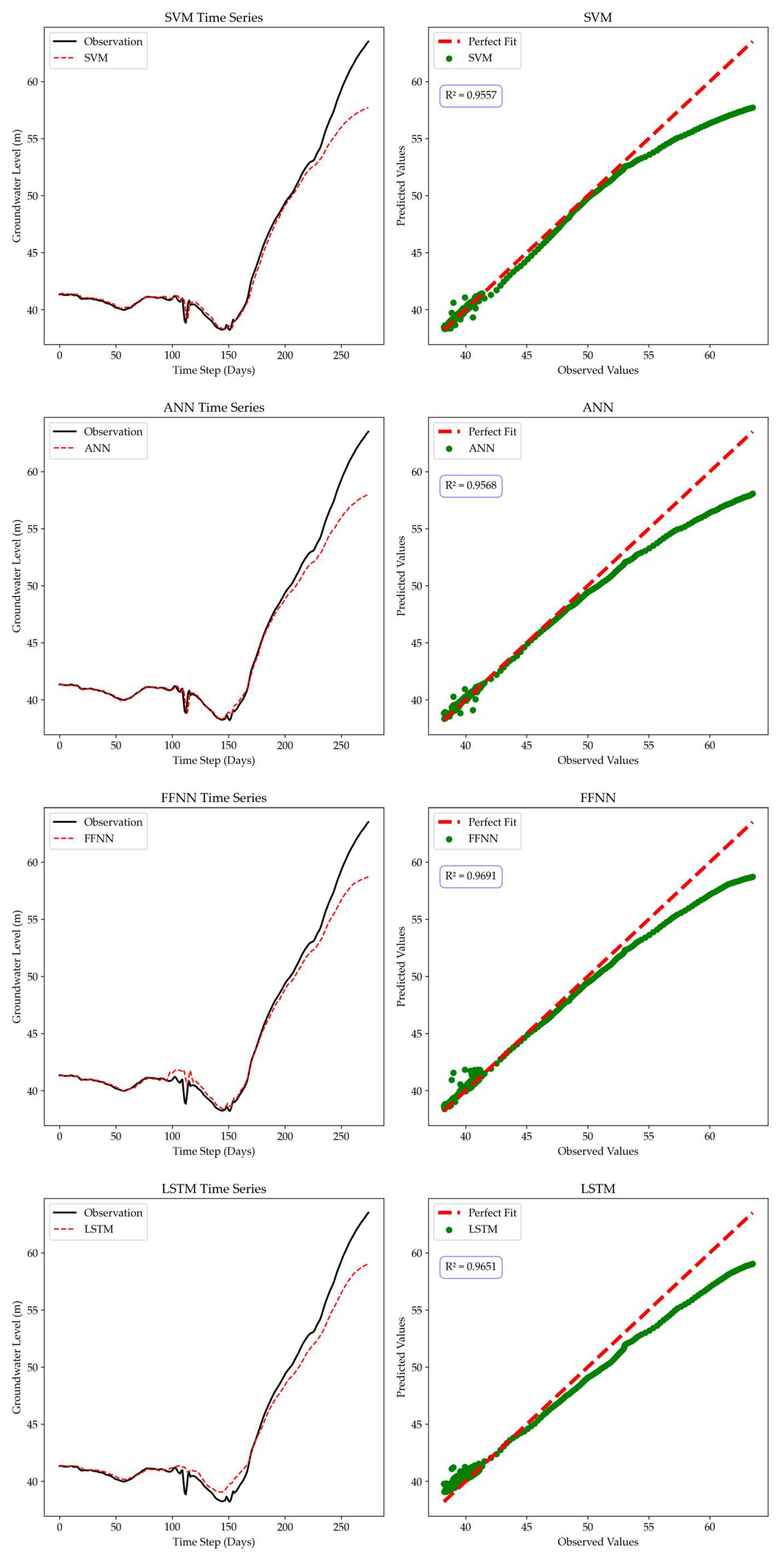
| ANN | 0.9995 | 0.9572 | 0.0060 | 0.0777 | 0.0636 | 0.7684 | 0.9995 | 0.9568 |
| FFNN | 0.9996 | 0.9692 | 0.0053 | 0.0638 | 0.0540 | 0.7219 | 0.9996 | 0.9691 |
| LSTM | 0.9986 | 0.9652 | 0.0105 | 0.0691 | 0.1099 | 0.8848 | 0.9986 | 0.9651 |
| GRU | 0.9996 | 0.9626 | 0.0053 | 0.0684 | 0.0554 | 0.6824 | 0.9996 | 0.9654 |
| ANFIS | 0.9996 | 0.9790 | 0.0055 | 0.0486 | 0.0557 | 0.6021 | 0.9996 | 0.9789 |
| NARX | 0.9994 | 0.9647 | 0.0069 | 0.0701 | 0.762 | 0.6782 | 0.9994 | 0.9646 |
| HGP | 0.9994 | 0.9933 | 0.0069 | 0.0259 | 0.0838 | 0.3758 | 0.9994 | 0.9933 |
| Removed Component | NSE | RMSE | MAE | R2 | ||||
|---|---|---|---|---|---|---|---|---|
| Train | Test | Train | Test | Train | Test | Train | Test | |
| Precipitation | 0.9993 | 0.9620 | 0.0071 | 0.0071 | 0.0732 | 0.8426 | 0.9993 | 0.9616 |
| Extraction | 0.9991 | 0.9687 | 0.0082 | 0.0632 | 0.0939 | 0.7042 | 0.9991 | 0.9685 |
| Policy | 0.9995 | 0.9726 | 0.0058 | 0.0599 | 0.0613 | 0.5702 | 0.9995 | 0.9725 |
| Above all | 0.9985 | 0.9577 | 0.0104 | 0.0777 | 0.1211 | 0.7597 | 0.9985 | 0.9574 |
| HGP | 0.9994 | 0.9933 | 0.0069 | 0.0259 | 0.0838 | 0.3758 | 0.9994 | 0.9933 |
Disclaimer/Publisher’s Note: The statements, opinions and data contained in all publications are solely those of the individual author(s) and contributor(s) and not of MDPI and/or the editor(s). MDPI and/or the editor(s) disclaim responsibility for any injury to people or property resulting from any ideas, methods, instructions or products referred to in the content. |
© 2023 by the authors. Licensee MDPI, Basel, Switzerland. This article is an open access article distributed under the terms and conditions of the Creative Commons Attribution (CC BY) license (https://creativecommons.org/licenses/by/4.0/).
Share and Cite
Zhang, J.; Dong, D.; Zhang, L. A New Method for Estimating Groundwater Changes Based on Optimized Deep Learning Models—A Case Study of Baiquan Spring Domain in China. Water 2023, 15, 4129. https://doi.org/10.3390/w15234129
Zhang J, Dong D, Zhang L. A New Method for Estimating Groundwater Changes Based on Optimized Deep Learning Models—A Case Study of Baiquan Spring Domain in China. Water. 2023; 15(23):4129. https://doi.org/10.3390/w15234129
Chicago/Turabian StyleZhang, Jialun, Donglin Dong, and Longqiang Zhang. 2023. "A New Method for Estimating Groundwater Changes Based on Optimized Deep Learning Models—A Case Study of Baiquan Spring Domain in China" Water 15, no. 23: 4129. https://doi.org/10.3390/w15234129