Addressing Nitrate Contamination in Groundwater: The Importance of Spatial and Temporal Understandings and Interpolation Methods

Abstract

Iranian water security is threatened by groundwater (GW) degradation. The excessive use of GW for agriculture in Iran is degrading these resources. Livestock waste disposal and sewage irrigation are also major contributors. Nitrate (NO₃) contamination in GW is a growing global concern, posing serious health and environmental risks. Soil can easily leach NO₃ into GW, causing long-term contamination. Understanding the temporal and spatial patterns of NO₃ pollution is vital in protecting human health and establishing safe drinking water limits. Choosing an appropriate interpolation method is crucial for creating a reliable spatial variability map, which is essential for environmental research and decision-making. This study used 85 GW samples collected over four periods to create interpolated maps and examine the spatial variability of NO₃ levels. Spatial interpolation methods were performed using the geostatistical tool within ArcGIS Software. The results showed that Empirical Bayesian Kriging (EBK) was the most effective of the five evaluated interpolation methods, although the performance of each method varied depending on the period sampled. Therefore, the choice of interpolation method should be tailored to the study’s specific needs and the characteristics of the data being interpolated. The EBK method produced interpolation maps that illustrated the spatial distribution of NO₃ concentrations, both within and exceeding the recommended guidelines. Interpolation methods can assist in creating spatial maps of NO₃ concentrations, identifying pollution sources, and developing targeted management strategies. These maps demonstrate the potential impact of human activities on the observed patterns. A thorough understanding of Iran’s current GW quality is very important and valuable for management and policymakers.

1. Introduction

Groundwater (GW) is the most reliable and accessible potable water source [1]. Many studies show that human activities compromise GW quality and public health [2,3,4,5,6]. With the intensification of agricultural and livestock farming in recent decades, there has been a corresponding increase in anthropogenic nitrogen (N) input, significantly impacting the global N cycle [7] and resulting in the widespread contamination of GW with nitrate (NO₃). Millions of people worldwide suffer from diseases caused by NO₃ contamination [8,9], such as colorectal cancer and thyroid disease [10,11,12,13]. NO₃ contamination is well-known in many areas, like Bangladesh, India, Algeria, Italy, and the Netherlands [14,15,16,17,18,19].

The issue of NO₃ contamination is a global concern, and Iran is no exception. The presence of more than 30 mg/L of NO₃ in water has been linked to several pollution sources, such as onsite sanitation, agricultural activities, and waste disposal [20,21,22,23]. The widespread use of nitrogen-based fertilisers in agriculture has been singled out as a significant source of NO₃ in the GW in agricultural regions. Livestock waste disposal and reusing sewage for irrigation are two other major contributors. Iran’s average nitrogen fertiliser application rate is over 200 kg Nha⁻¹ [24]. In regions where high-yielding crops are grown, the nitrogen fertiliser application rate often exceeds 300 kg Nha⁻¹ [25]. Livestock waste disposal and reusing sewage for irrigation are two other major contributors.

In Iran, the NO₃ levels range from 0.1 to 428 mg/L, with the highest levels in the Kurdistan province [26]. The Fars and Tehran provinces have also reported relatively high levels of NO₃ [26,27]. The situation in Iran may be more complex due to the unique hydrogeological environment and increasing expansion of agricultural activities.

However, this high level of nitrogen input can lead to decreased utilisation efficiency and contamination of GW and surface water, which can negatively impact human health and aquatic ecosystems [28,29]. The studies highlight the potential for NO₃ contamination in both surface and GW sources in various regions of Iran and the need for continued monitoring and management practices to ensure safe water resources for human consumption and ecological health. As such, an urgent need exists to understand the composition, source, and contribution ratio of nitrogen to effectively control NO₃ pollution from the transportation of nitrogen into GW. To address this issue, the government of Iran has implemented various policies and regulations, including promoting sustainable agriculture practices and developing wastewater treatment plants [30]. Nevertheless, further research is needed to address the issue of NO₃ contamination, particularly in light of increasing agricultural intensity and its potential impact on the country’s water resources.

One way to study GW contamination is through a Geographic Information System (GIS) used for visualising environmental contaminant spatial distribution [31,32,33]. However, due to time and money constraints, fewer GW samples are collected in the field for chemical analysis, which could impact experimental results and findings [34]. To fill gaps in the conceptual site model, interpolating isolated well data can predict values at unsampled locations using nearby measured values [35]. Inverse Distance Weighting (IDW), Kriging, and Empirical Bayesian Kriging are three common interpolation methods used for mapping GW contamination [36,37]. However, there are still differences of opinion regarding the accuracy of contamination interpolating under different conditions for different pollutants. For example, Saha et al. [38] compared the performance of IDW, Ordinary Kriging (OK), and Radial Basis Functions (RBF) to map the spatial distribution of arsenic contamination. They indicated that the RBF model was the best for interpolation prediction and could ensure the accurate fitting of predicted data with measured data at sampling sites. Based on the relative performance of four interpolation methods, the best methods for interpolating GW quality parameters were Empirical Bayesian Kriging (EBK) for pH, TDS, SO₄, and NO₃, and OK for nickel and hardness [39]. Previously, interpolation methods were used to investigate the spatial distribution of NO₃. Koussa and Berhail [40] examined different interpolation methods to predict the NO₃ concentration data from 305 wells in the synclinal of Algeria. The analysis showed that the kriging methods performed better, showing greater consistency in the predicted NO₃ concentration, fewer interpolation errors, and lower biases. Mukherjee and Singh [41] found that OK and EBK, compared to several kriging models, performed best for high rain and low rainy seasons to interpolate the NO₃ variations in India. Interpolation accuracy depends on sampling design, population size, boundary demarcation, and data set normality, affecting applicability [42,43,44,45].

Our research compares, describes, and predicts the performance of various interpolation methods in mapping regional NO₃ concentrations due to the urgent need to understand and address NO₃ contamination. This method lets us see the problem’s scope. This study will improve our understanding of spatial and temporal NO₃ contamination trends and help us choose the best interpolation method for future research and remediation. Our ultimate goal is to strengthen pollution control and environmental protection strategies.

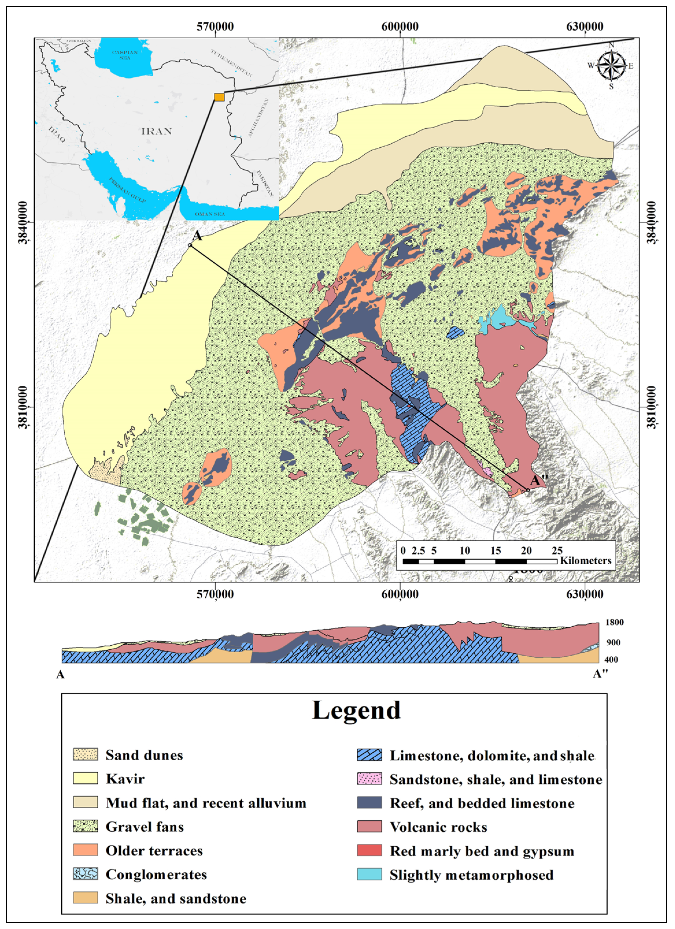
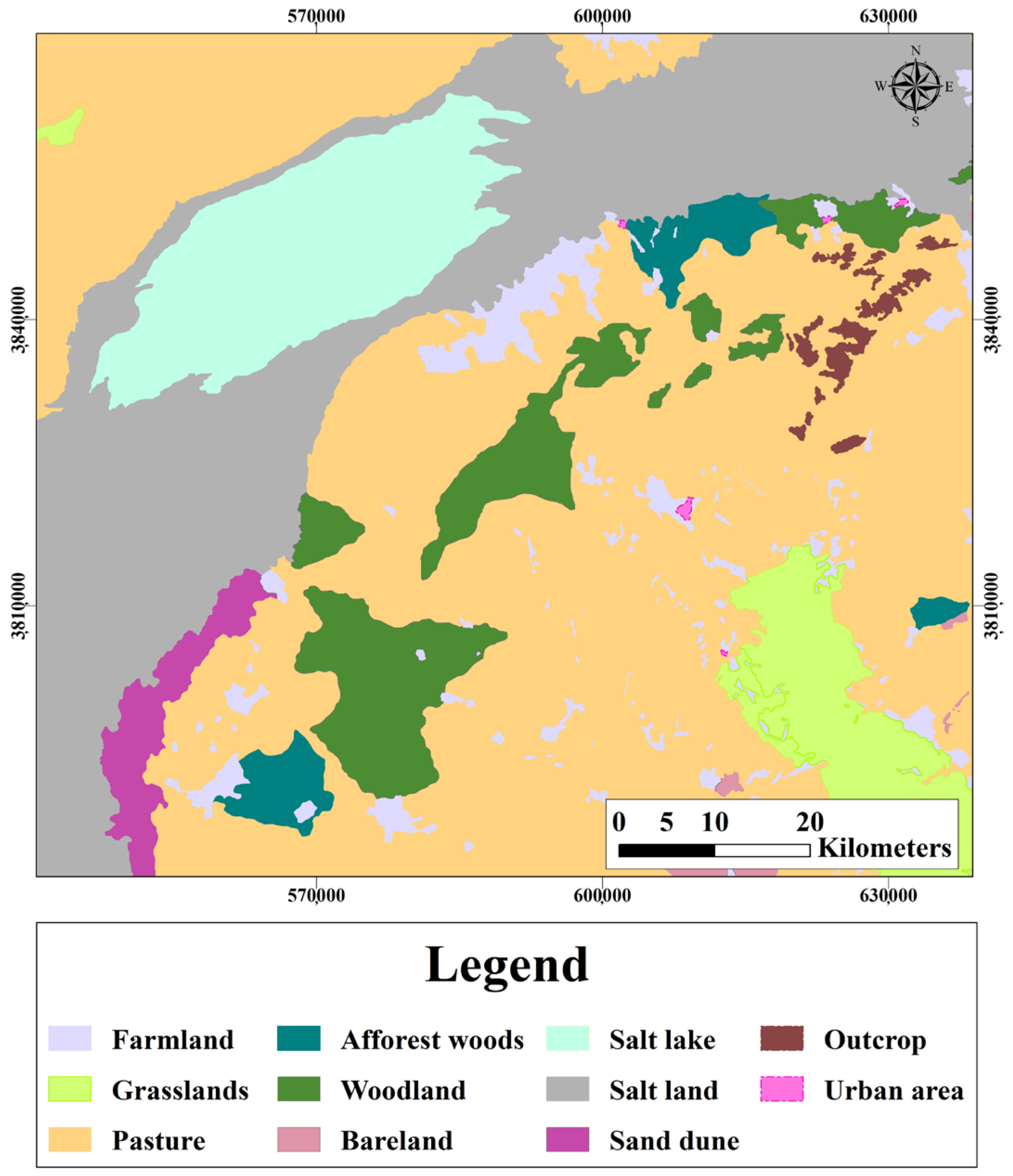
2. Study Area, Hydrology and Hydrogeology Setting

The Bajestan and Yunusi basins, located south of the Khorasan Razavi province in eastern Iran, have been studied due to the high levels of NO₃ in the GW in some areas. The study area has an arid climate, receiving only 149–155 millimetres of annual rainfall and having an average annual temperature of 16.4–17.3 degrees Celsius. The region’s geology is dominated by sedimentary rocks, including sandstone, shale, and limestone, deposited during the Mesozoic and Cenozoic eras. These sedimentary rocks are generally tilted with dips towards the east and southeast (Figure 1) [46]. The primary GW source in these basins is the alluvial deposits of the Quaternary age, consisting of unconsolidated sediments, such as sand, gravel, and clay [47]. The recharge rates are low, ranging from 2 to 5 mm/year, and the aquifer parameters, such as hydraulic conductivity, transmissivity, and storativity, have been determined through extensive hydrogeological studies [47,48]. The hydraulic conductivity ranges from 10 to 150 m/day, indicating the sediments’ high permeability and the aquifer’s ability to transmit water [46].

Due to low rainfall, high surface water salinity, and electrical conductivity, most of the area’s water needs are met by wells and qanats. At the same time, only a small amount comes from springs (Figure 2) [49]. However, the GW potential is decreasing due to several factors, including the low potential precipitation, the expansion of cultivated land, the growing population, and recent droughts. The study area has many small farms, and farmers use nitrogenous fertilisers and manure to enhance agricultural output (Figure 3). Furthermore, as Qasemi et al. [50] mentioned, almost all of the inhabitants in the area use unprotected wells for their wastewater disposal, which increases the risk of NO₃ contamination.

3. Materials and Methods

3.1. Interpolation and Spatial Analysis

This study evaluated NO₃ contamination using various interpolation methods to identify spatial changes in 2022. To accomplish this, the research was divided into two stages: data collection, processing, and analysis using ArcMap 10.8 (provided by Utrecht University), followed by comparing and evaluating spatial interpolation models to select the most effective method. To carry out the analysis, IPI, IDW, OK, UK, and EBK interpolations were calculated and analysed using ArcMap 10.8, and NO₃ interpolation maps were generated using the ArcMap 10.8 Geostatistical Wizard. This study utilised a dataset consisting of 85 samples collected from the Bajestan and Yunusi aquifers to identify the interpolation method that best explains the spatial changes in GW quality. The Khorasan Razavi Regional Water Company collected datasets comprising physicochemical parameters of GW samples, which encompassed measurements of electrical conductivity (EC), pH, and temperature, as well as concentrations of Ca, Mg, Na, HCO₃, SO₄, NO₃, and Cl. The data were collected during the period spanning from January to December. The predominant hydrochemical composition of the GW in the study area is primarily characterised as Na-Cl type [51]. The pH values exhibited a range spanning from 7 to 9.5. The mean total hardness of the irrigation wells was approximately 10.3. The electrical conductivity (EC) values observed in the wells exhibited a range of 602 to 17,450 µS/cm, with an average value of 5912 µS/cm. According to the World Health Organisation (WHO) [52], the maximum permissible EC value is 1500 µS/cm. Therefore, it can be observed that the conductivity in the majority of the wells surpasses the permissible threshold.

Table 1. Descriptive statistics for the collected GW samples.

	Minimum	Maximum	Mean	Standard Deviation	Variance
EC	602	17,450	5919	4634	21,469,697
pH	7	8.66	7.69	0.28	0.08
HCO3	0.2	8	3	1	1
Cl	1.1	148	40	39	1496
SO4	1.1	47	14	10	91
Mg	0.5	49	5	6	41
Na	0.4	145	48	38	1416
NO3	4.6	153	49	39	1504

shows the descriptive statistics pertaining to the collected data. However, our primary focus is NO₃ among the various parameters presented.

Parameters were adjusted using the Geostatistical Analyst (GA) to verify the model and approach the best interpolation for each technique. Finally, interpolation maps were created, and the interpolation surfaces were transformed from GA layers into Rasters using the Raster tool (Figure 4).

3.2. Interpolation Methods

In our current study, we have employed the five interpolation techniques that are most commonly used, as identified through a review of the literature [53,54,55]. We will briefly overview each method in this context and highlight its most significant distinctions.

3.2.1. LPI Method

The LPI method is a powerful interpolation technique widely used in various applications, including GW-quality mapping. Unlike other interpolation methods, the LPI method employs a linear regression model with varying regression coefficients, which allows for assessing the dependence of the desired variable on data locations. It fits a local polynomial using point regression coefficients only within the specified neighbourhood, resulting in surfaces that capture short-range variation with a variable relief form [56,57]. This method is computationally efficient and easy to implement, making it suitable for real-time applications with limited resources [58]. However, it assumes that the signal is linear and that the noise in the data is small. The LPI interpolation method’s general Equation (1) can estimate the signal value at any intermediate time point by linearly interpolating between adjacent data points using the slope of the straight line that passes through them.

$$z_i=y\left(s_i\right)+{\epsilon }_i=X\left(s_i\right)\beta \left(s\right)+{\epsilon }_i$$

(1)

where $z_i$ is the estimated value of the unknown point at the location $s_i$. $y\left(s_i\right)$ is the true value of the dependent, ${\epsilon }_i$ is the residual error, $X\left(s_i\right)$ is a matrix of independent variables, and β(s) is a vector of regression coefficients at location $s_i$.

The LPI interpolation method maps regularly collected data from GW monitoring networks, especially in heterogeneous areas.

3.2.2. IDW

The IDW interpolation method is another popular technique used for GW-quality mapping. IDW stands for Inverse Distance Weighting, which means that the method calculates the interpolated values based on the weighted average of the measured values from the nearest neighbouring data points. The weight of each point is determined based on its distance from the interpolated point, with closer points having a higher weight than those farther away. This method is often used when the spatial distribution of data is uneven and the data points are unevenly spaced. The IDW interpolation method is easy to implement and computationally efficient, making it suitable for large datasets. However, it assumes that the underlying data is continuous and no abrupt changes exist. The general equation for the IDW interpolation method can estimate the value at any point by using the following formula (Equation (2)).

$$Z(x,y)=\sum \left[Zi/{\left(\mathrm{distance}\right)}^p\right]/\sum \left[1/{\left(\mathrm{distance}\right)}^p\right]$$

(2)

where Z(x,y) is the estimated value at a given point, $Zi$ is the measured value at the $i$_th location, and p is the power parameter used to control the influence of the distance on the weights. The IDW interpolation method can produce surfaces that capture long-range variation but may not be suitable for capturing short-range variation as the method needs to consider the spatial relationships between the data points.

3.2.3. Classical Kriging Methods

Classical Kriging is a powerful geostatistical technique used to predict the value of a regional variable at unsampled locations based on measured data. As a set of linear regression routines, it assumes that the variable can be considered regional, meaning that it varies continuously and has a certain degree of spatial correlation between nearby points. The method relies on variograms, which describe the spatial correlation of the variable at different distances. By contracting the variogram from the measured data ($\widehat{m}$), the predicted value ($\widehat{z}$) at an unsampled location (s₀) can be estimated. The spatial trend and random components can be added using the semivariogram $\left(\widehat{e}\right)$. The variogram range presents the distance at which spatial correlation vanishes, indicating the maximum distance at which points can be considered statistically independent. Different kriging techniques, such as OK and UK, are employed based on these variables to obtain robust predictions (Equation (3)).

$$\widehat{z}\left(s_0\right)=\widehat{m}\left(s_0\right)+\widehat{e}\left(s_0\right)$$

(3)

• OK

Ordinary Kriging (OK) is a geostatistical technique commonly used for spatial prediction. It computes optimal weights based on the semivariogram of the data and assigns weights to measured points to predict values at unsampled locations [59]. OK also incorporates a location-dependent mean that can vary from one point to another. This makes OK estimation robust even when the stationarity condition is violated. OK assumes a quasi-stationarity condition, meaning the covariance is considered constant while the mean can vary [60,61]. Therefore, OK can assume that there is mean stationarity within the kriging search neighbourhood (2). This allows for more accurate predictions in situations where the mean of the studied variable varies over space (Equation (4)).

$$\widehat{z}\left(s_0\right)={\sum }_{\mathrm{i}=1}^{\mathrm{n}} {\mathrm{w}}_{\mathrm{i}}{d}_{\mathrm{i}}$$

(4)

where $\widehat{z}\left(s_0\right)$ represents the estimated value at the unsampled location $s_0$, $\mathrm{n}$ represents the number of data locations available for the variable being studied, $d_{\mathrm{i}}$ is the known value at location i in the study area, and ${\mathrm{w}}_{\mathrm{i}}$ represents the weight assigned to location $\mathrm{i}$ based on the model semivariogram.

• SK

According to Viswanathan et al. [62], SK differs from OK in that it employs the global mean of the complete dataset and subsequently incorporates estimated residuals. The equation for UK can be expressed as Equation (5).

$$\widehat{z}\left(s_0\right)=\mathrm{m}+{\sum }_{\mathrm{i}=1}^{\mathrm{n}} {\lambda }_{\mathrm{i}}\left[d_{\mathrm{i}}-\mathrm{m}\right]$$

(5)

The weight assigned for location $\mathrm{i}$ is represented by ${\lambda }_{\mathrm{i}}$, and the average value derived from the sample variance is denoted by $\mathrm{m}$.

• UK

Universal Kriging (UK) is another geostatistical technique commonly used for spatial prediction. Like Ordinary Kriging, UK also uses a location-dependent mean, but instead of assuming a constant mean, UK calculates the mean using a multi-order polynomial [63]. The estimated residual is then added to provide a more precise result. The equation for UK can be expressed as Equation (6).

$$\widehat{z}\left(s_0\right)={\sum }_{i=1}^N {\lambda }_{i}Z\left(d_i\right)$$

(6)

where ${\lambda }_i$ represents the weight assigned to location $i$ and $Z\left(d_i\right)$ represents the observed values at points $d_i$, found from the sample variance.

The main difference between UK and OK is that UK does not assume stationarity and does not remove trends [59]. Instead, UK calculates the mean using a polynomial and then estimates the residual to provide a more accurate result. Additionally, UK requires prior knowledge of the covariates and parameters, while OK does not. In summary, UK estimates the mean using a polynomial while both UK and OK use a location-dependent mean. It estimates the residual, whereas OK assumes a constant mean and removes trends.

If a polynomial function can capture the trend component of the spatial variation, then LPI is equivalent to Universal Kriging. However, if the spatial trend is more complex than can be described by a polynomial, then the UK model may provide more accurate results. A detailed discussion on the relationship between classical kriging methods and deterministic interpolation methods, such as LPI, can be found in the literature, including Krivoruchko [64] and Li and Heap [65].

3.2.4. EBK

The EBK interpolation method stands out from other classical kriging approaches because it uses a system that automatically optimises several semivariogram models rather than relying on a single semivariogram [66,67] and manual parameter adjustments [58,66]. By assuming variations at location i, (z) are statistically homogeneous across the surface, and EBK predicts values at specified locations using a limited number of nearest observations. To generate these semivariograms automatically, EBK uses a process of subsetting and simulations. This allows the algorithm to create a regression kriging model that bends to prior local trends when the data coverage is insufficient [68,69]. Multiple data subsets, including those with different trends, can contribute to the prediction results. The final distribution map is created by combining the results of the local models [67,70]. Overall, EBK is a solid non-stationary algorithm for spatiotemporal interpolation and is often the best of all geostatistical models for interpolating GW data. The general equation for EBK is (Equation (7)):

$$Z\left(u\right)=\sum (i=1 \mathrm{to} n)\lambda i\left(u\right)Zi$$

(7)

where $Z\left(u\right)$ is the estimated value at location $u$, $Zi$ is the known value at sample location i, n is the number of sample points, and $\lambda i\left(u\right)$ is the kriging weight assigned to each sample point i at location $u$.

The kriging weight $\lambda i\left(u\right)$ is calculated using (Equation (8)):

$$\lambda \mathrm{i}\left(\mathrm{u}\right)=\mathrm{w}\mathrm{i}\left(\mathrm{u}\right)/\sum (\mathrm{j}=1 \mathrm{to} \mathrm{n})\mathrm{w}\mathrm{j}\left(\mathrm{u}\right)$$

(8)

where $\mathrm{w}\mathrm{i}\left(\mathrm{u}\right)$ is the weight assigned to sample point $\mathrm{i}$ at location $\mathrm{u}$ and is calculated using (Equation (9)):

$$\mathrm{w}\mathrm{i}\left(u\right)=1/\left(vi\right(u)+\mathsf{\tau }2)$$

(9)

where $vi\left(u\right)$ is the estimated local variance at location $u,$ and $\mathsf{\tau }$ is the estimation error variance.

3.3. Interpolation and Validation

In this study, ArcMap 10.8 was used to apply various tasks to the data. The geostatistical wizard within ArcMap was utilised to adjust the parameter configurations for optimal interpolation methods. NO₃ concentrations decreased first-order across the study site. To adhere to kriging’s assumption that there should be no global trends in the dataset, the first-order trend was removed from the three interpolation methods [59,71,72]. Furthermore, NO₃ concentrations were not normally distributed, were corrected in the OK and EBK interpolation models using a log transformation [73,74], and were confirmed using the Geostatistical Wizard’s Quantile–Quantile (QQ) Plots. We used the exponential kernel function and the semivariogram function type in the OK interpolation method. All other variables were kept at their standard values while optimising the interpolation model for fit and accuracy. For EBK interpolation, log empirical transformation and the exponential semivariogram model were used; all other settings were kept as default. Improved operational efficiency and accuracy were gained by keeping the semivariogram power at 100 simulations [75]. For IDW interpolation, the weighting power was set to one because it showed the lowest RMSE. This means that, for the NO₃ data, points farther away can still have a significant effect on the predictions [76].

The leave-one-out cross-validation (LOOCV) technique is well-established for evaluating interpolation accuracy in hydrogeological studies [77,78]. LOOCV systematically removes each point in the interpolation, predicts its value by interpolating the remaining points, and compares the expected value to the measured value [76,78]. This method provides reliable and widely accepted results by providing Root Mean Squared Error (RMSE) and Mean Absolute Error (MAE) values. The lowest value of RMSE determines the most appropriate interpolation method [60,79]. The mean value is also employed to detect any bias or smoothing effects introduced by cross-validation errors. In addition, Nash–Sutcliffe Efficiency (NSE) is a statistical measure used to evaluate the accuracy of a hydrological model’s predictions. It is based on comparing modelled discharge with observed data, and the resulting efficiency values can range from negative infinity to 1. An efficiency value of 1 indicates a perfect match between the model’s predictions and the observed data [76,80]. In contrast, a value of 0 suggests that the model predictions are as accurate as the mean of the observed data. However, when the efficiency value is less than zero, it indicates that the observed mean is a better predictor than the model, implying that the model’s residual variance is larger than the data variance. In essence, the closer the efficiency value is to 1, the more accurate the model’s predictions are, and the closer it is to 0, the less accurate the model becomes. As a result, the RMSE, MAE, and NSE were calculated with the following Equation (10) to (13) to assess the performance of different interpolation methods.

$$\mathrm{RMSE}=\sqrt{\frac{1}{n}{\sum }_{i=1}^n{\left[Z\left(x_i\right)-Z^{*}\left(x_i\right)\right]}^2}$$

(10)

$$\mathrm{MAE}=\frac{{\sum }_{i=1}^n\left|Z^{*}\left(x_i\right)-Z\left(x_i\right)\right|}{n}$$

(11)

$$\mathrm{NSE}=1-\frac{{\sum }_{i=1}^n\left[{\left(z\left(x_i\right)-Z^{*}\left(x_i\right)\right]}^2\right.}{{\sum }_{i=1}^n \left[{\left(z\left(x_i\right)-O\right]}^2\right.}$$

(12)

where $z\left(x_i\right)$, and $Z^{*}\left(x_i\right)$ are the observed and interpolated values of the NO₃ concentration of the i_th well, $n$ is the number of observations, and $O$ is the mean of these values.

4. Results and Discussion

4.1. Measured NO₃ Concentrations

NO₃ is a common contaminant found in GW that can pose health risks to humans and animals if present in excessive amounts. To ensure safe drinking water, different countries and organisations have established various classifications and limits for NO₃ levels. The Environmental Protection Agency has set a maximum contaminant level of 10 mg/L for NO₃ in drinking water in the United States [81]. In comparison, the WHO recommends a limit of 50 mg/L for NO₃ in drinking water [52]. Similarly, in Europe, the European Union has set a limit of 50 mg/L for NO₃ in drinking water and has established GW quality standards for NO₃ levels that vary by country [82]. Per Iranian guidelines, NO₃ concentration should not surpass 50 mg/L. Additionally, nitrite (NO₂) is recognised as another crucial indicator. When compared to their respective standard values, the sum ratio of each of these elements should not exceed one [83]. These classifications and limits ensure that NO₃ levels in GW remain within safe and acceptable levels for human consumption and environmental protection.

Table 2. Common implementation strategy for NO₃ in drinking water.

Purpose	Proper (mg/L)	Good (mg/L)	Fair (mg/L)	Poor
Drinking Water Quality	<10	10–20	20–50	>50

presents the common implementation strategy for NO₃ in drinking water based on WHO’s recommendations [52].

Table 3. NO₃ concentration and WHO classification across sampling periods.

Sampling Periods	WHO Classification	Count	NO3 Concentration (mg/L)
			Minimum	Mean ± SD	Maximum
Spring	Good	1	15	15.3	15
	Fair	7	23	25.6 ± 2.6	31
	Poor	7	80	111 ± 26	153
Summer	Fair	11	24	34 ± 9	49
	Poor	8	75	105.2 ± 24.9	148
Autumn	Excellent	1	5	4.6	5
	Good	4	12	15.7 ± 2.9	19
	Fair	15	22	27.8 ± 6.5	47
	Poor	7	55	101.9 ± 27.5	140
Winter	Good	2	15	16 ± 1.1	17
	Fair	12	21	29.9 ± 7.1	41
	Poor	6	57	107.8 ± 28.5	142

presents the temporal patterns observed among the NO₃ concentrations across the study area (cf. Table 1). The table shows the number of wells in each category and the minimum, mean ± SD, and maximum NO₃ concentration (mg/L) for each category.

In the Spring sampling period, only one well had a Good water quality classification with an NO₃ concentration of 15 mg/L. Seven wells were classified as Fair, with a mean NO₃ concentration of 25.6 mg/L and a maximum concentration of 31 mg/L. The Poor category had the highest count of wells (80), with a mean NO₃ concentration of 111 mg/L and a maximum concentration of 153 mg/L. During the summer, 11 wells were classified as Fair, with a mean NO₃ concentration of 34 mg/L and a maximum concentration of 49 mg/L. Eight wells were classified as Poor, with a mean NO₃ concentration of 105.2 mg/L and a maximum concentration of 148 mg/L.

In the Autumn sampling period, one well was classified as Excellent, with a NO₃ concentration of 4.6 mg/L. Four wells were classified as Good, with a mean NO₃ concentration of 15.7 mg/L and a maximum concentration of 19 mg/L. Fifteen wells were classified as Fair, with a mean NO₃ concentration of 27.8 mg/L and a maximum concentration of 47 mg/L. Seven wells were classified as Poor, with a mean NO₃ concentration of 101.9 mg/L and a maximum concentration of 140 mg/L. During the Winter sampling period, two wells were classified as Good, with a mean NO₃ concentration of 16 mg/L and a maximum concentration of 17 mg/L. Twelve wells were classified as Fair, with a mean NO₃ concentration of 29.9 mg/L and a maximum concentration of 41 mg/L. Six wells were classified as Poor, with a mean NO₃ concentration of 107.8 mg/L and a maximum concentration of 142 mg/L.

The data show that the NO₃ concentrations in the study area varied widely across the sampling periods. The presence of a significant temporal pattern in our study area compounds the importance of spatial patterns. High NO₃ concentration levels consistently exceed 40 mg/L, posing an ongoing threat to human health and the environment. Interpolation methods play a critical role in generating spatial maps that pinpoint the areas most affected by agricultural activities and identify the sources of NO₃ pollution. Armed with this crucial information, we can develop targeted management strategies to reduce the harmful effects of NO₃ pollution and mitigate its impact over time.

Moreover, by highlighting farming activities, such as fertiliser use and animal waste management, as the primary contributors to high NO₃ levels in water sources, interpolation can raise awareness among stakeholders and farmers about the severity of NO₃ pollution. Encouraging behavioural changes towards more sustainable farming practices, like adopting improved fertiliser application techniques and better animal waste management, is crucial to addressing the problem.

The interpolation of NO₃ concentration in water sources is essential for protecting human health and the environment. By creating spatial maps of NO₃ concentration, we can identify high-risk areas and implement effective management strategies to reduce NO₃ pollution in our study area. A combination of public education campaigns and targeted management strategies can also promote behavioural changes among stakeholders and farmers, leading to sustainable agriculture practices that safeguard the environment and human health.

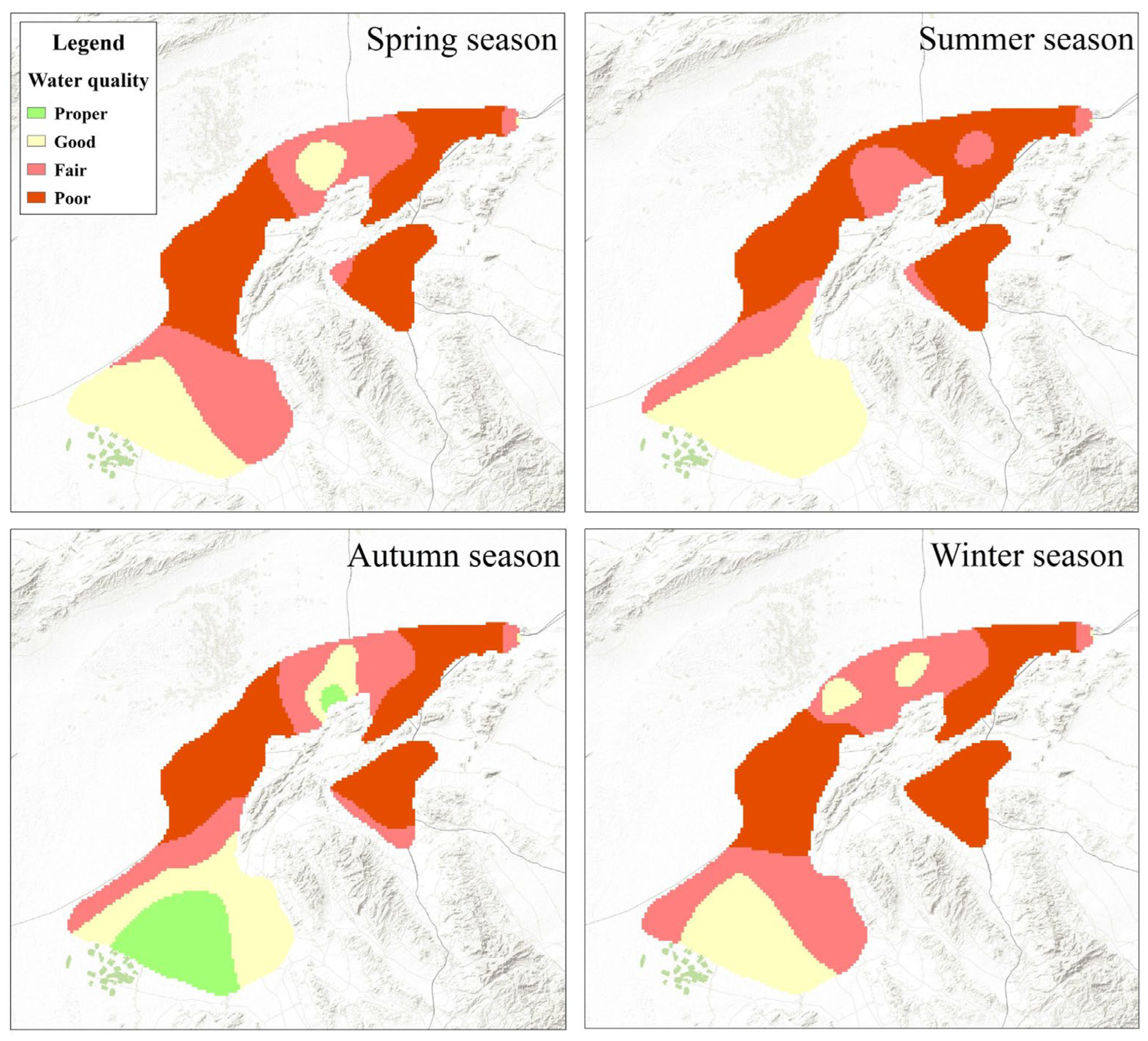
4.2. Visualisation of Prediction

NO₃ is a prevalent form of groundwater contamination on a global scale [84]. Its transfer from surface waters can exacerbate water quality issues and harm ecosystems [85]. The spatial distribution of NO₃ in the analysed area was demonstrated using the IDW, LPI, UK, OK, and EBK methodologies and displayed significant variations in overall accuracy due to over or underestimation. The parameters’ values obtained in this study exhibit spatial variability, as reported by previous researchers [86]. Nevertheless, all five techniques predicted that the highest NO₃ values would be concentrated in the northeast and central regions (Figure 5). The observed outcome could be attributed to applying mineral fertilisers and the local topography, which enables the movement of nitrate-contaminated water across the surface and subsurface. The significant reduction in nitrates in the grassland can be attributed to the extensive uptake of nitrate forms, mainly due to plants’ high solubility and easy absorption of nitrates. The diminished presence of nitrogen in the grassland may have been attributed to the decrease in nitrification processes, which can be attributed to elevated groundwater levels and a reduced thickness of the aeration zone in the lower regions. At the same time, lower levels (around or below 20 mg/L) were mainly found in the southern part of the study area. Several potential factors may have exerted influence in this context. One possible explanation for this phenomenon is the absence of vegetation in the field, which may lead to heightened mineralisation processes of organic matter in plant remnants and residues after mineral fertilisation.

Second, in desert regions, the NO₃ concentration in GW can vary significantly, particularly during autumn. This variation can be attributed to a multitude of factors. One of the critical factors is the scarcity of nitrate sources in these areas, especially during the summer when these sources are not utilised. Moreover, human activities such as agriculture, which often involve nitrate-rich fertilisers, are typically reduced during this period. This reduction, coupled with the low levels of rainfall—a primary vehicle for nitrate transport into groundwater—results in a significant decrease in nitrate infiltration [87]. The physical properties of desert soils, which are predominantly sandy and exhibit low water retention, further impede the transport of nitrates into the groundwater. Notably, nitrate transport from surface water to groundwater is not instantaneous but instead is dictated by the hydraulic flow, which requires time [88,89]. This time-dependent process could explain why the lowest nitrate concentrations are observed in the autumn, as the process commences in the summer but takes time to manifest in the groundwater nitrate levels. Therefore, the nitrate concentration in the groundwater reflects the cumulative effects of these seasonal and environmental factors.

Examining the spatial distribution of NO₃ in groundwater or soil has garnered considerable interest within environmental studies in recent times. Although the research literature has extensively examined various aspects of the subject, there has been a lack of focus on comparing prediction accuracy. In their study, Hong et al. [90] employed two methodologies, OK and IDW interpolation, to illustrate groundwater NO₃’s spatial distribution effectively. Bernard-Jannin et al. [91] employed the Inverse IDW method to assess the spatial and temporal fluctuations of denitrification rates within a floodplain region. A limited number of scholarly articles have addressed the quantitative evaluation of the precision of various spatial interpolation methods. Prominent instances encompass the works of Kazemi et al. [92] and Bronowicka et al. [93]. The research conducted by Kazemi et al. [92] holds significant relevance in this context. The present study assessed the performance of four geostatistical methods, namely IDW, spline, natural neighbour, and OK, in estimating nitrate concentration levels in groundwater. The evaluation of the accuracy of each method was conducted using MRE, RMSE, and %RMSE (percentage root mean square error) as the criteria. The study’s results indicated that the spline and natural neighbour methods yielded more precise estimations than the IDW and OK methods. In summary, using geostatistical methods demonstrated superior fitting performance compared to deterministic methods. Although no universally superior method was identified, the most precise outcomes were obtained using the Co-OK approach.

4.3. Cross-Validation Analyses

The given table provides a comparison of different interpolation methods based on their statistical indices for four different seasons. To evaluate the overall performance of each method, the mean and standard deviation of the three statistical indices, namely RMSE, Mean CV, and NSE, were calculated (

Table 4. Statistical results of each interpolation method for each sampling period in the study. Interpolation methods used. RMSE, MAE, NSE, and Mean CV are shown.

Interpolation Method	Statistical Indices	Spring	Summer	Autumn	Winter
LPI	RMSE	47.3	31.6	30.5	38.8
	Mean CV	5.1	3	0.68	0.94
	NSE	0.017	0.098	0.282	0.076
IDW	RMSE	37.6	36.9	28.2	35.4
	Mean CV	−1.9	3.43	−2.54	−2.41
	NSE	0.117	0.093	0.081	0.028
OK	RMSE	37.6	34.3	28.05	33.05
	Mean CV	1.19	−1.03	−0.44	1.89
	NSE	0.015	0.043	0.032	0.148
SK	RMSE	43.1	39.7	35.5	40.1
	Mean CV	−0.93	0.55	2.1	0.137
	NSE	0.186	0.173	0.193	0.185
UK	RMSE	−0.93	44.3	37.8	42.9
	Mean CV	2.15	−1.03	−0.66	1.68
	NSE	0.085	0.093	0.091	0.014
EBK	RMSE	28.6	26.5	28.1	30.63
	Mean CV	1.4	−0.76	−0.72	0.1
	NSE	0.223	0.166	0.189	0.192

). The LPI method has a mean RMSE of 36.55 and a standard deviation of 7.93, a mean Mean CV of 2.93 and a standard deviation of 2.21, and a mean NSE of 0.118 with a standard deviation of 0.106. The IDW method has a mean RMSE of 34.28 with a standard deviation of 4.05, a mean Mean CV of −0.9 and a standard deviation of 2.52, and a mean NSE of 0.08 with a standard deviation of 0.032. The OK method has a mean RMSE of 33.25 and a standard deviation of 3.37, a mean Mean CV of 0.4 and a standard deviation of 1.26, and a mean NSE of 0.06 with a standard deviation of 0.058. The SK method has a mean RMSE of 39.6 and a standard deviation of 2.49, a mean Mean CV of 0.47 and a standard deviation of 1.2, and a mean NSE of 0.182 with a standard deviation of 0.008. The UK method has a mean RMSE of 31.56 and a standard deviation of 38.37, a mean Mean CV of 0.78 and a standard deviation of 1.47, and a mean NSE of 0.071 with a standard deviation of 0.032. Finally, the EBK method has a mean RMSE of 28.72 with a standard deviation of 1.62, a mean Mean CV of 0.03 and a standard deviation of 1.01, and a mean NSE of 0.193 with a standard deviation of 0.023.

Looking at the RMSE values, we can see that EBK had the lowest error for all four seasons, followed by IDW and OK. LPI had the highest RMSE values for all seasons, indicating it had the poorest performance among the methods. The IDW method had negative Mean CV values for all seasons, suggesting that it tended to underestimate the values. LPI had positive Mean CV values for all seasons, indicating that it tended to overestimate them. SK had positive Mean CV values for Spring and Winter and negative Mean CV values for Summer and Autumn, indicating that it overestimated values in the former and underestimated them in the latter. UK had positive Mean CV values for spring and negative values for the other three seasons. EBK had negative Mean CV values for Summer, Autumn, and Winter, indicating that it tended to underestimate the values.

Looking at the NSE values, we can see that SK had the highest NSE values for all seasons except for Winter, where EBK had the highest value. LPI had the lowest NSE values for all seasons, indicating the poorest performance among the methods. The table shows that SK and EBK performed better than the other methods, while LPI performed poorly. However, it is important to note that the performance of each method varied depending on the season, with some methods performing better in certain seasons than others.

5. Conclusions

This research aimed to assess different interpolation methods and identify the most accurate one for point estimations. This is crucial for understanding NO₃ concentrations in groundwater and ensuring the safety of drinking water. The study emphasises the importance of understanding the temporal and spatial patterns of NO₃ pollution. Interpolation methods are vital in creating spatial maps to locate pollution sources and develop targeted management strategies. These methods can also raise awareness among stakeholders and farmers about the severity of NO₃ pollution, encouraging a move towards more sustainable farming practices.

The Empirical Bayesian Kriging (EBK) method is the most effective overall among the five interpolation methods evaluated, according to the statistical indices presented. However, it is important to remember that the effectiveness of each method changes with the season, and no single method consistently performs the best throughout the year. As a result, the choice of an interpolation method should be customised to the study’s specific needs and the characteristics of the data being interpolated.

There is not a one-size-fits-all approach to choosing an interpolation type. Creating the most accurate representation of spatial variability for a given characteristic should always start with selecting an interpolation method. The initial selection of interpolation method should consider sample sizes, sampling types, and data distribution. After performing specific interpolations, the best method can be selected based on relevant statistical error measures.

References

1. Zaresefat, M.; Derakhshani, R. Revolutionizing Groundwater Management with Hybrid AI Models: A Practical Review. Water 2023, 15, 1750. [Google Scholar] [CrossRef]
2. Rezaei, A.; Hassani, H.; Hassani, S.; Jabbari, N.; Fard Mousavi, S.B.; Rezaei, S. Evaluation of Groundwater Quality and Heavy Metal Pollution Indices in Bazman Basin, Southeastern Iran. Groundw. Sustain. Dev. 2019, 9, 100245. [Google Scholar] [CrossRef]
3. Rezaei, A.; Hassani, H.; Jabbari, N. Evaluation of Groundwater Quality and Assessment of Pollution Indices for Heavy Metals in North of Isfahan Province, Iran. Sustain. Water Resour. Manag. 2019, 5, 491–512. [Google Scholar] [CrossRef]
4. Mammeri, A.; Tiri, A.; Belkhiri, L.; Salhi, H.; Brella, D.; Lakouas, E.; Tahraoui, H.; Amrane, A.; Mouni, L. Assessment of Surface Water Quality Using Water Quality Index and Discriminant Analysis Method. Water 2023, 15, 680. [Google Scholar] [CrossRef]
5. Tiri, A.; Lahbari, N.; Boudoukha, A. Hydrochemical Characterization of Surface Water in the Timgad Watershed, East Algeria. Desalination Water Treat. 2016, 57, 562–571. [Google Scholar] [CrossRef]
6. Zaresefat, M.; Derakhshani, R.; Nikpeyman, V.; GhasemiNejad, A.; Raoof, A. Using Artificial Intelligence to Identify Suitable Artificial Groundwater Recharge Areas for the Iranshahr Basin. Water 2023, 15, 1182. [Google Scholar] [CrossRef]
7. Galloway, J.N.; Townsend, A.R.; Erisman, J.W.; Bekunda, M.; Cai, Z.; Freney, J.R.; Martinelli, L.A.; Seitzinger, S.P.; Sutton, M.A. Transformation of the Nitrogen Cycle: Recent Trends, Questions, and Potential Solutions. Science 2008, 320, 889–892. [Google Scholar] [CrossRef]
8. Wu, J.; Sun, Z. Evaluation of Shallow Groundwater Contamination and Associated Human Health Risk in an Alluvial Plain Impacted by Agricultural and Industrial Activities, Mid-West China. Expo Health 2016, 8, 311–329. [Google Scholar] [CrossRef]
9. He, S.; Wu, J. Hydrogeochemical Characteristics, Groundwater Quality, and Health Risks from Hexavalent Chromium and Nitrate in Groundwater of Huanhe Formation in Wuqi County, Northwest China. Expo. Health 2019, 11, 311–329. [Google Scholar] [CrossRef]
10. Childs, D.B. Water Source and Thyroid Disease Mortality in Georgia. ABNF J. 2020, 31, 127–131. [Google Scholar]
11. Ward, M.H.; Jones, R.R.; Brender, J.D.; de Kok, T.M.; Weyer, P.J.; Nolan, B.T.; Villanueva, C.M.; van Breda, S.G. Drinking Water Nitrate and Human Health: An Updated Review. Int. J. Environ. Res. Public Health 2018, 15, 1557. [Google Scholar] [CrossRef]
12. World Health Organization. WHO Guidelines for Drinking-Water Quality; World Health Organization: Geneva, Switzerland, 2011; Volume 216, pp. 303–304.
13. Xi, Y.; Xu, P. Global Colorectal Cancer Burden in 2020 and Projections to 2040. Transl. Oncol. 2021, 14, 101174. [Google Scholar] [CrossRef]
14. Ahmed, N.; Bodrud-Doza, M.; Towfiqul Islam, A.R.M.; Hossain, S.; Moniruzzaman, M.; Deb, N.; Bhuiyan, M.A.Q. Appraising Spatial Variations of As, Fe, Mn and NO3 Contaminations Associated Health Risks of Drinking Water from Surma Basin, Bangladesh. Chemosphere 2019, 218, 726–740. [Google Scholar] [CrossRef]
15. Busico, G.; Kazakis, N.; Colombani, N.; Mastrocicco, M.; Voudouris, K.; Tedesco, D. A Modified SINTACS Method for Groundwater Vulnerability and Pollution Risk Assessment in Highly Anthropised Regions Based on NO3 and SO42− Concentrations. Sci. Total Environ. 2017, 609, 1512–1523. [Google Scholar] [CrossRef] [PubMed]
16. Nejatijahromi, Z.; Nassery, H.R.; Hosono, T.; Nakhaei, M.; Alijani, F.; Okumura, A. Groundwater Nitrate Contamination in an Area Using Urban Wastewaters for Agricultural Irrigation under Arid Climate Condition, Southeast of Tehran, Iran. Agric. Water Manag. 2019, 221, 397–414. [Google Scholar] [CrossRef]
17. Griffioen, J.; Vermooten, S.; Janssen, G. Geochemical and Palaeohydrological Controls on the Composition of Shallow Groundwater in the Netherlands. Appl. Geochem. 2013, 39, 129–149. [Google Scholar] [CrossRef]
18. Severini, E.; Bartoli, M.; Pinardi, M.; Celico, F. Reactive Silica Traces Manure Spreading in Alluvial Aquifers Affected by Nitrate Contamination: A Case Study in a High Plain of Northern Italy. Water 2020, 12, 2511. [Google Scholar] [CrossRef]
19. Brella, D.; Belkhiri, L.; Tiri, A.; Salhi, H.; Lakouas, F.E.; Nouibet, R.; Amrane, A.; Merdoud, R.; Mouni, L. Identification of the Groundwater Quality and Potential Noncarcinogenic Health Risk Assessment of Nitrate in the Groundwater of El Milia Plain, Kebir Rhumel Basin, Algeria. Hydrology 2023, 10, 171. [Google Scholar] [CrossRef]
20. He, X.; Wu, J.; He, S. Hydrochemical Characteristics and Quality Evaluation of Groundwater in Terms of Health Risks in Luohe Aquifer in Wuqi County of the Chinese Loess Plateau, Northwest. Hum. Ecol. Risk Assess. Int. J. 2018, 25, 32–51. [Google Scholar] [CrossRef]
21. Yu, L.; Zheng, T.; Zheng, X.; Hao, Y.; Yuan, R. Nitrate Source Apportionment in Groundwater Using Bayesian Isotope Mixing Model Based on Nitrogen Isotope Fractionation. Sci. Total Environ. 2020, 718, 137242. [Google Scholar] [CrossRef]
22. Kazakis, N.; Matiatos, I.; Ntona, M.M.; Bannenberg, M.; Kalaitzidou, K.; Kaprara, E.; Mitrakas, M.; Ioannidou, A.; Vargemezis, G.; Voudouris, K. Origin, Implications and Management Strategies for Nitrate Pollution in Surface and Ground Waters of Anthemountas Basin Based on a δ15N -NO3− and δ18O- -NO3− Isotope Approach. Sci. Total Environ. 2020, 724, 138211. [Google Scholar] [CrossRef] [PubMed]
23. Ahada, C.P.S.; Suthar, S. Groundwater Nitrate Contamination and Associated Human Health Risk Assessment in Southern Districts of Punjab, India. Environ. Sci. Pollut. Res. 2018, 25, 25336–25347. [Google Scholar] [CrossRef] [PubMed]
24. Jalali, M. Nitrates Leaching from Agricultural Land in Hamadan, Western Iran. Agric. Ecosyst. Environ. 2005, 110, 210–218. [Google Scholar] [CrossRef]
25. Solgi, E.; Jalili, M. Zoning and Human Health Risk Assessment of Arsenic and Nitrate Contamination in Groundwater of Agricultural Areas of the Twenty Two Village with Geostatistics (Case Study: Chahardoli Plain of Qorveh, Kurdistan Province, Iran). Agric. Water Manag. 2021, 255, 107023. [Google Scholar] [CrossRef]
26. Bahrami, M.; Zarei, A.R.; Rostami, F. Temporal and Spatial Assessment of Groundwater Contamination with Nitrate by Nitrate Pollution Index (NPI) and GIS (Case Study: Fasarud Plain, Southern Iran). Environ. Geochem. Health 2020, 42, 3119–3130. [Google Scholar] [CrossRef] [PubMed]
27. Ghahremanzadeh, H.; Noori, R.; Baghvand, A.; Nasrabadi, T. Evaluating the Main Sources of Groundwater Pollution in the Southern Tehran Aquifer Using Principal Component Factor Analysis. Environ. Geochem. Health 2017, 40, 1317–1328. [Google Scholar] [CrossRef]
28. Badrzadeh, N.; Samani, J.M.V.; Mazaheri, M.; Kuriqi, A. Evaluation of Management Practices on Agricultural Nonpoint Source Pollution Discharges into the Rivers under Climate Change Effects. Sci. Total Environ. 2022, 838, 156643. [Google Scholar] [CrossRef]
29. Karavidas, I.; Ntatsi, G.; Vougeleka, V.; Karkanis, A.; Ntanasi, T.; Saitanis, C.; Agathokleous, E.; Ropokis, A.; Sabatino, L.; Tran, F.; et al. Agronomic Practices to Increase the Yield and Quality of Common Bean (Phaseolus vulgaris L.): A Systematic Review. Agronomy 2022, 12, 271. [Google Scholar] [CrossRef]
30. Foroushani, T.S.; Balali, H.; Movahedi, R.; Kurban, A.; Värnik, R.; Stamenkovska, I.J.; Azadi, H. Importance of Good Groundwater Governance in Economic Development: The Case of Western Iran. Groundw. Sustain. Dev. 2023, 21, 100892. [Google Scholar] [CrossRef]
31. Ehteshami, M.; Salari, M.; Zaresefat, M. Sustainable Development Analyses to Evaluate Groundwater Quality and Quantity Management. Model. Earth Syst. Environ. 2016, 2, 133. [Google Scholar] [CrossRef]
32. Zaresefat, M.; Kalantari, N.; Aram, E.; Rouhi, H. Potential for Natural Feeding of Groundwater Using FAHP Method and GIS Software. In Proceedings of the Thirtieth Meeting of Earth Sciences, Tehran, Iran, 16 May 2011; pp. 1–5. [Google Scholar]
33. Zaresefat, M.; Ahrari, M.; Reza Shoaei, G.; Etemadifar, M.; Aghamolaie, I.; Derakhshani, R. Identification of Suitable Site-Specific Recharge Areas Using Fuzzy Analytic Hierarchy Process (FAHP) Technique: A Case Study of Iranshahr Basin (Iran). Air Soil Water Res. 2022, 15, 1–12. [Google Scholar] [CrossRef]
34. Liu, C.W.; Jang, C.S.; Liao, C.M. Evaluation of Arsenic Contamination Potential Using Indicator Kriging in the Yun-Lin Aquifer (Taiwan). Sci. Total Environ. 2004, 321, 173–188. [Google Scholar] [CrossRef]
35. Freitag, P.; Martac, E.; Reichenauer, T. On the Effectiveness of Site Investigation in Regard to Project Costs—A Case Study. Ce/papers 2018, 2, 439–444. [Google Scholar] [CrossRef]
36. Bhunia, G.S.; Shit, P.K.; Maiti, R. Comparison of GIS-Based Interpolation Methods for Spatial Distribution of Soil Organic Carbon (SOC). J. Saudi Soc. Agric. Sci. 2018, 17, 114–126. [Google Scholar] [CrossRef]
37. Murphy, R.R.; Curriero, F.C.; Ball, W.P. Comparison of Spatial Interpolation Methods for Water Quality Evaluation in the Chesapeake Bay. J. Environ. Eng. 2010, 136, 160–171. [Google Scholar] [CrossRef]
38. Saha, A.; Gupta, B.S.; Patidar, S.; Martínez-Villegas, N. Spatial Distribution Based on Optimal Interpolation Techniques and Assessment of Contamination Risk for Toxic Metals in the Surface Soil. J. S. Am. Earth Sci. 2022, 115, 103763. [Google Scholar] [CrossRef]
39. Amah, V.E.; Agu, F.A. Geostatistical Modelling of Groundwater Quality at Rumuola Community, Port Harcourt, Nigeria. Asian J. Environ. Ecol. 2020, 12, 37–47. [Google Scholar] [CrossRef]
40. Koussa, M.; Berhail, S. Evaluation of Spatial Interpolation Techniques for Mapping Groundwater Nitrates Concentrations—Case Study of Ain Elbel-Sidi Makhlouf Syncline in The Djelfa Region (Algeria). LARHYSS 2021, 45, 119–140. [Google Scholar]
41. Mukherjee, I.; Singh, U.K. Characterization of Groundwater Nitrate Exposure Using Monte Carlo and Sobol Sensitivity Approaches in the Diverse Aquifer Systems of an Agricultural Semiarid Region of Lower Ganga Basin, India. Sci. Total Environ. 2021, 787, 147657. [Google Scholar] [CrossRef]
42. Güler, M.; Kara, T. Comparison of Different Interpolation Techniques for Modelling Temperatures in Middle Black Sea Region. J. Agric. Fac. Gaziosmanpasa Univ. 2014, 31, 61–71. [Google Scholar] [CrossRef]
43. Hengl, T. A Practical Guide to Geostatistical Mapping, 2nd ed.; EUR 22904 EN Scientific and Technical Research Series; Office for Official Publications of the European Communities: Luxembourg, 2009. [Google Scholar]
44. Stahl, K.; Moore, R.D.; Floyer, J.A.; Asplin, M.G.; McKendry, I.G. Comparison of Approaches for Spatial Interpolation of Daily Air Temperature in a Large Region with Complex Topography and Highly Variable Station Density. Agric. For. Meteorol. 2006, 139, 224–236. [Google Scholar] [CrossRef]
45. Wu, W.; Tang, X.-P.; Ma, X.-Q.; Liu, H.-B. A Comparison of Spatial Interpolation Methods for Soil Temperature over a Complex Topographical Region. Theor. Appl. Climatol. 2016, 125, 657–667. [Google Scholar] [CrossRef]
46. Majid Padashi, S.; Büdel, C.; Ullmann, T.; Tintrup, A.; Baumhauer, R.; Majid Padashi, S.; Büdel, C.; Ullmann, T.; Tintrup, A.; Baumhauer, R. Preliminary Results on Quaternary Studies from Bajestan Basin (Kavir-e Namak), Iran. EGUGA 2017, 19, 16532. [Google Scholar]
47. Nematollahi, M.J.; Ebrahimi, P.; Ebrahimi, M. Evaluating Hydrogeochemical Processes Regulating Groundwater Quality in an Unconfined Aquifer. Environ. Process. 2016, 3, 1021–1043. [Google Scholar] [CrossRef]
48. Dehghani, M.H.; Zarei, A.; Yousefi, M.; Asgharia, F.B.; Haghighat, G.A. Fluoride Contamination in Groundwater Resources in the Southern Iran and Its Related Human Health Risks. Desalination Water Treat. 2019, 153, 95–104. [Google Scholar] [CrossRef]
49. Mohammadzadeh, F.; Ekhtesasi, M.R.; Hosseini, S.Z.; Negaresh, A.; Hashemi, H.; Allaee, M. Investigating the Effect of Drinking and Sanitary Water Separation on the Quality of Drinking Water and Preparing a Groundwater Quality Map (Case Study: Bajestan Watershed). J. Watershed Manag. Res. 2022, 13, 215–229. [Google Scholar] [CrossRef]
50. Qasemi, M.; Afsharnia, M.; Farhang, M.; Bakhshizadeh, A.; Allahdadi, M.; Zarei, A. Health Risk Assessment of Nitrate Exposure in Groundwater of Rural Areas of Gonabad and Bajestan, Iran. Environ. Earth Sci. 2018, 77, 551. [Google Scholar] [CrossRef]
51. Mohammadzadeh, F.; Ekhtesasi, M.R.; Hosseini, S.Z. The Effects of Geological Formations on Groundwater Quality with the Application of Boolean Logic, Case Study: Bajestan Watershed Plain. Watershed Eng. Manag. 2017, 9, 11–21. [Google Scholar]
52. WHO. Nitrate and Nitrite in Drinking-Water Background Document for Development of WHO Guidelines for Drinking-Water Quality; WHO/FWC/WSH/16.52; World Health Organization: Geneva, Switzerland, 2016.
53. de Smith, M.J.; Goodchild, M.F.; Longley, P. Geospatial Analysis: A Comprehensive Guide to Principles, Techniques and Software Tools, 6th ed.; Troubador Publishing Ltd.: Market Harborough, UK, 2021; ISBN 9781912556038. [Google Scholar]
54. Webster, R.; Oliver, M.A. Geostatistics for Environmental Scientists; John Wiley & Sons: Hoboken, NJ, USA, 2007; ISBN 0470517263. [Google Scholar]
55. Smith, J.E.; von Winterfeldt, D. Decision Analysis in Management Science. Manag. Sci. 2004, 50, 561–574. [Google Scholar] [CrossRef]
56. Hani, A.; Abari, S.A.H. Determination of Cd, Zn, K, PH, TNV, Organic Material and Electrical Conductivity (EC) Distribution in Agricultural Soils Using Geostatistics and GIS (Case Study: South–Western of Natanz–Iran). Int. J. Biol. Life Agric. Sci. 2011, 12, 852–855. [Google Scholar] [CrossRef]
57. Gribov, A.; Krivoruchko, K. Local Polynomials for Data Detrending and Interpolation in the Presence of Barriers. Stoch. Environ. Res. Risk Assess. 2011, 25, 1057–1063. [Google Scholar] [CrossRef]
58. Esri. ArcGIS Geostatistical Analyst—Model Spatial Data & Uncertainty. Available online: https://www.esri.com/en-us/arcgis/products/geostatistical-analyst/overview (accessed on 9 November 2021).
59. Paramasivam, C.R.; Venkatramanan, S. An Introduction to Various Spatial Analysis Techniques. In GIS and Geostatistical Techniques for Groundwater Science; Elsevier: Amsterdam, The Netherlands, 2019; pp. 23–30. ISBN 9780128154137. [Google Scholar]
60. Lange, J.; Krause, E. Spatial Interpolation with ArcGIS Pro—Esri Training Seminar. 2019. Available online: https://www.esri.com/training/catalog/5c92b940fa73df28264fb8ed/spatial-interpolation-with-arcgis-pro (accessed on 22 June 2022).
61. Esri. ArcMap—Documentation. Available online: https://desktop.arcgis.com/en/arcmap/latest/tools/spatial-analyst-toolbox/conditional-evaluation-with-con.htm (accessed on 27 November 2021).
62. Viswanathan, R.; Jagan, J.; Samui, P.; Porchelvan, P. Spatial Variability of Rock Depth Using Simple Kriging, Ordinary Kriging, RVM and MPMR. Geotech. Geol. Eng. 2015, 33, 69–78. [Google Scholar] [CrossRef]
63. Abdulmanov, R.; Miftakhov, I.; Ishbulatov, M.; Galeev, E.; Shafeeva, E. Comparison of the Effectiveness of GIS-Based Interpolation Methods for Estimating the Spatial Distribution of Agrochemical Soil Properties. Environ. Technol. Innov. 2021, 24, 101970. [Google Scholar] [CrossRef]
64. Krivoruchko, K. Spatial Statistical Data Analysis for GIS Users, 1st ed.; Esri Press: Redlands, CA, USA, 2011; ISBN 978-1-58948-161-9. [Google Scholar]
65. Li, J.; Heap, A.D. Spatial Interpolation Methods Applied in the Environmental Sciences: A Review. Environ. Model. Softw. 2014, 53, 173–189. [Google Scholar] [CrossRef]
66. Krivoruchko, K. Empirical Bayesian Kriging. ArcUser Fall 2012, 6, 1145. [Google Scholar]
67. Gribov, A.; Krivoruchko, K. Empirical Bayesian Kriging Implementation and Usage. Sci. Total Environ. 2020, 722, 137290. [Google Scholar] [CrossRef] [PubMed]
68. Knotters, M.; Heuvelink, G.B.M. A Disposition of Interpolation Techniques; Wettelijke Onderzoekstaken Natuur & Milieu: Wageningen, The Netherlands, 2010. [Google Scholar]
69. Krivoruchko, K.; Butler, K. Unequal Probability-Based Spatial Mapping; Esri: Redlands, CA, USA, 2013. [Google Scholar]
70. Krivoruchko, K.; Gribov, A. Distance Metrics for Data Interpolation over Large Areas on Earth’s Surface. Spat. Stat. 2020, 35, 100396. [Google Scholar] [CrossRef]
71. de Gans, W.; Wong, T.E.; Batjes, D.A.J.; de Jager, J. Geology of the Netherlands; Royal Netherlands Academy of Arts and Sciences: Amsterdam, The Netherlands, 2007. [Google Scholar]
72. Jarmołowski, W.; Wielgosz, P.; Ren, X.; Krypiak-Gregorczyk, A. On the Drawback of Local Detrending in Universal Kriging in Conditions of Heterogeneously Spaced Regional TEC Data, Low-Order Trends and Outlier Occurrences. J. Geod. 2021, 95, 2. [Google Scholar] [CrossRef]
73. Gong, G.; Mattevada, S.; O’Bryant, S.E. Comparison of the Accuracy of Kriging and IDW Interpolations in Estimating Groundwater Arsenic Concentrations in Texas; Elsevier: Amsterdam, The Netherlands, 2014. [Google Scholar]
74. Singh, P.; Verma, P. A Comparative Study of Spatial Interpolation Technique (IDW and Kriging) for Determining Groundwater Quality. GIS Geostat. Tech. Groundw. Sci. 2019, 43–56. [Google Scholar] [CrossRef]
75. Tomlinson, K.M. A Spatial Evaluation of Groundwater Quality Salinity and Underground Injection Controlled Wells Activity in Texas. Ph.D. Thesis, The University of Texas at Dallas, Richardson, TX, USA, 2019. [Google Scholar]
76. Xie, Y.; Chen, T.; Lei, M.; Yang, J.; Guo, Q.; Song, B.; Zhou, X. Spatial Distribution of Soil Heavy Metal Pollution Estimated by Different Interpolation Methods: Accuracy and Uncertainty Analysis. Chemosphere 2011, 82, 468–476. [Google Scholar] [CrossRef]
77. Ahmad, A.Y.; Saleh, I.A.; Balakrishnan, P.; Al-Ghouti, M.A. Comparison GIS-Based Interpolation Methods for Mapping Groundwater Quality in the State of Qatar. Groundw. Sustain. Dev. 2021, 13, 100573. [Google Scholar] [CrossRef]
78. Mirzaei, R.; Sakizadeh, M. Comparison of Interpolation Methods for the Estimation of Groundwater Contamination in Andimeshk-Shush Plain, Southwest of Iran. Environ. Sci. Pollut. Res. 2016, 23, 2758–2769. [Google Scholar] [CrossRef]
79. Krause, E. Model Water Quality Using Interpolation. Available online: https://learn.arcgis.com/en/projects/model-water-quality-using-interpolation (accessed on 15 February 2023).
80. Wagner, P.D.; Fiener, P.; Wilken, F.; Kumar, S.; Schneider, K. Comparison and Evaluation of Spatial Interpolation Schemes for Daily Rainfall in Data Scarce Regions. J. Hydrol. 2012, 464–465, 388–400. [Google Scholar] [CrossRef]
81. EPA. Drinking Water Requirements for States and Public Water Systems. Available online: https://www.epa.gov/dwreginfo/drinking-water-regulations (accessed on 4 April 2023).
82. EU Guidance Common Implementation Strategy for the Water Framework Directive (2000/60/EC); European Environment Agency: Copenhagen, Denmark, 2003; Volume 7.
83. Institute of Standards and Industrial Research of Iran. Drinking Water—Physical and Chemical Specifications; Institute of Standards and Industrial Research of Iran: Tehran, Iran, 2010. [Google Scholar]
84. Spalding, R.F.; Exner, M.E. Occurrence of Nitrate in Groundwater—A Review. J. Environ. Qual. 1993, 22, 392–402. [Google Scholar] [CrossRef]
85. Boesch, D.F.; Brinsfield, R.B.; Magnien, R.E. Chesapeake Bay Eutrophication: Scientific Understanding, Ecosystem Restoration, and Challenges for Agriculture. J. Environ. Qual. 2001, 30, 303–320. [Google Scholar] [CrossRef] [PubMed]
86. Kennedy, C.D.; Genereux, D.P.; Corbett, D.R.; Mitasova, H. Spatial and Temporal Dynamics of Coupled Groundwater and Nitrogen Fluxes through a Streambed in an Agricultural Watershed. Water Resour. Res. 2009, 45, W09401. [Google Scholar] [CrossRef]
87. Ki, M.-G.; Koh, D.-C.; Yoon, H.; Kim, H. Temporal Variability of Nitrate Concentration in Groundwater Affected by Intensive Agricultural Activities in a Rural Area of Hongseong, South Korea. Environ. Earth Sci. 2015, 74, 6147–6161. [Google Scholar] [CrossRef]
88. Wells, M.J.; Gilmore, T.E.; Nelson, N.; Mittelstet, A.; Böhlke, J.K. Determination of Vadose Zone and Saturated Zone Nitrate Lag Times Using Long-Term Groundwater Monitoring Data and Statistical Machine Learning. Hydrol. Earth Syst. Sci. 2021, 25, 811–829. [Google Scholar] [CrossRef]
89. Turkeltaub, T.; Kurtzman, D.; Dahan, O. Real-Time Monitoring of Nitrate Transport in the Deep Vadose Zone under a Crop Field—Implications for Groundwater Protection. Hydrol. Earth Syst. Sci. 2016, 20, 3099–3108. [Google Scholar] [CrossRef]
90. Hong, N.; White, J.G.; Weisz, R.; Gumpertz, M.L.; Duffera, M.G.; Cassel, D.K. Groundwater Nitrate Spatial and Temporal Patterns and Correlations: Influence of Natural Controls and Nitrogen Management. Vadose Zone J. 2007, 6, 53–66. [Google Scholar] [CrossRef]
91. Bernard-Jannin, L.; Sun, X.; Teissier, S.; Sauvage, S.; Sánchez-Pérez, J.M. Spatio-Temporal Analysis of Factors Controlling Nitrate Dynamics and Potential Denitrification Hot Spots and Hot Moments in Groundwater of an Alluvial Floodplain. Ecol. Eng. 2017, 103, 372–384. [Google Scholar] [CrossRef]
92. Kazemi, E.; Karyab, H.; Emamjome, M.-M. Optimisation of Interpolation Method for Nitrate Pollution in Groundwater and Assessing Vulnerability with IPNOA and IPNOC Method in Qazvin Plain. J. Environ. Health Sci. Eng. 2017, 15, 23. [Google Scholar] [CrossRef] [PubMed]
93. Bronowicka-Mielniczuk, U.; Mielniczuk, J.; Obroślak, R.; Przystupa, W. A Comparison of Some Interpolation Techniques for Determining Spatial Distribution of Nitrogen Compounds in Groundwater. Int. J. Environ. Res. 2019, 13, 679–687. [Google Scholar] [CrossRef]
Figure 1. The surface geology of the study area.
Water 15 04220 g001
Figure 2. The distribution of samples, springs, qanats, and irrigation wells.
Water 15 04220 g002
Figure 3. The land use of the study area. Note that the pasture unit also refers to dryland farming.
Water 15 04220 g003
Figure 4. The flowchart schematic illustrates the process of identifying the most suitable interpolation method.
Water 15 04220 g004
Figure 5. This diagram represents the spatial distribution of NO3 across four distinct seasons, according to WHO classification. The distribution patterns were determined using the optimal method.
Water 15 04220 g005