
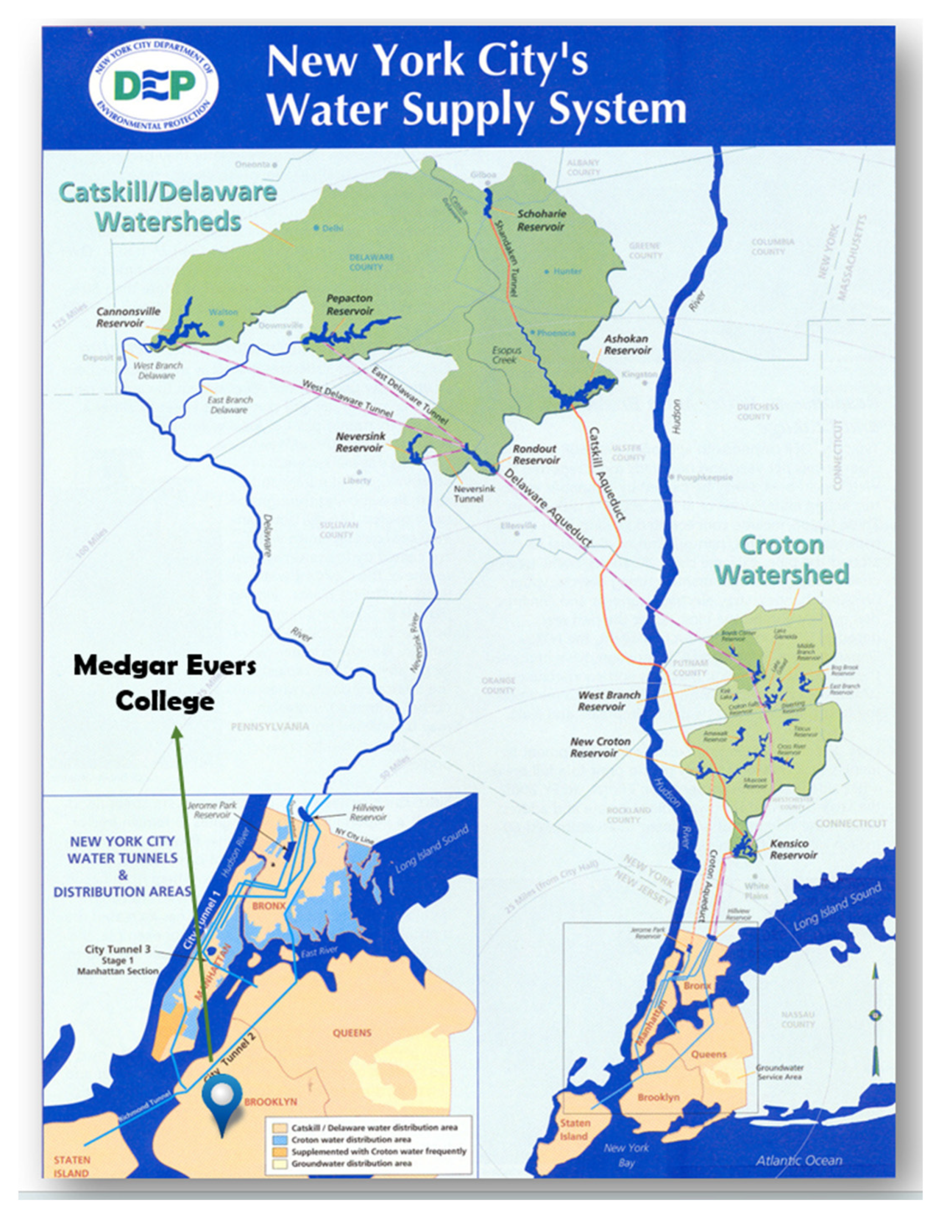
Environmental Assessment and Monitoring of Heavy Metals in New York City Potable Water Systems: Case Study at Medgar Evers College, Correlation Analysis, and Public Health Impacts


 ,
, 
 ,
, 
Abstract
:1. Introduction
2. Experimental Methodology
2.1. Water Sample Preparation and Storage
2.2. ICP-MS Analysis
2.3. Sample Quality Control
3. Results and Discussion
3.1. Iron (Fe)
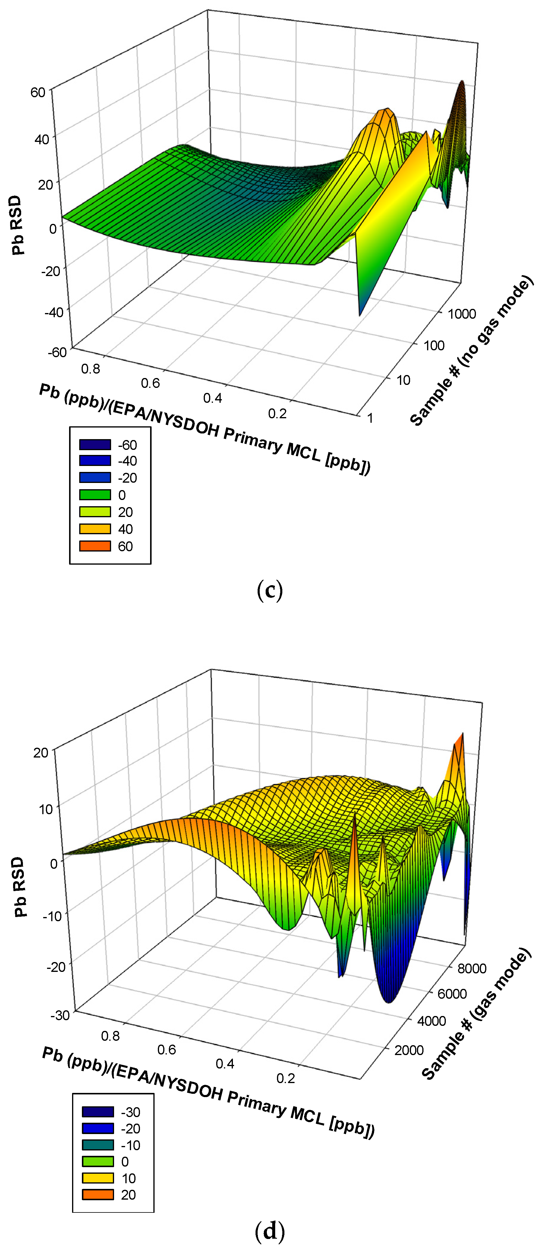
3.2. Lead (Pb)
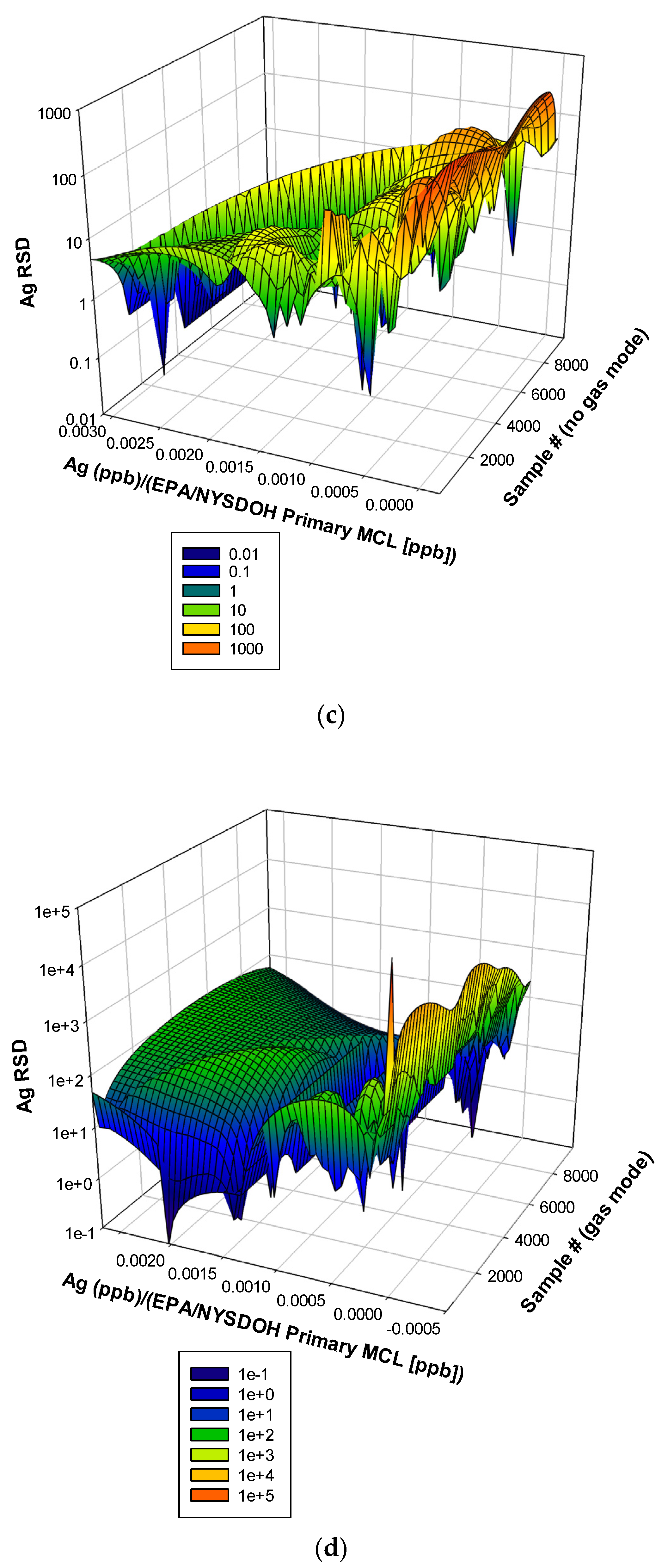
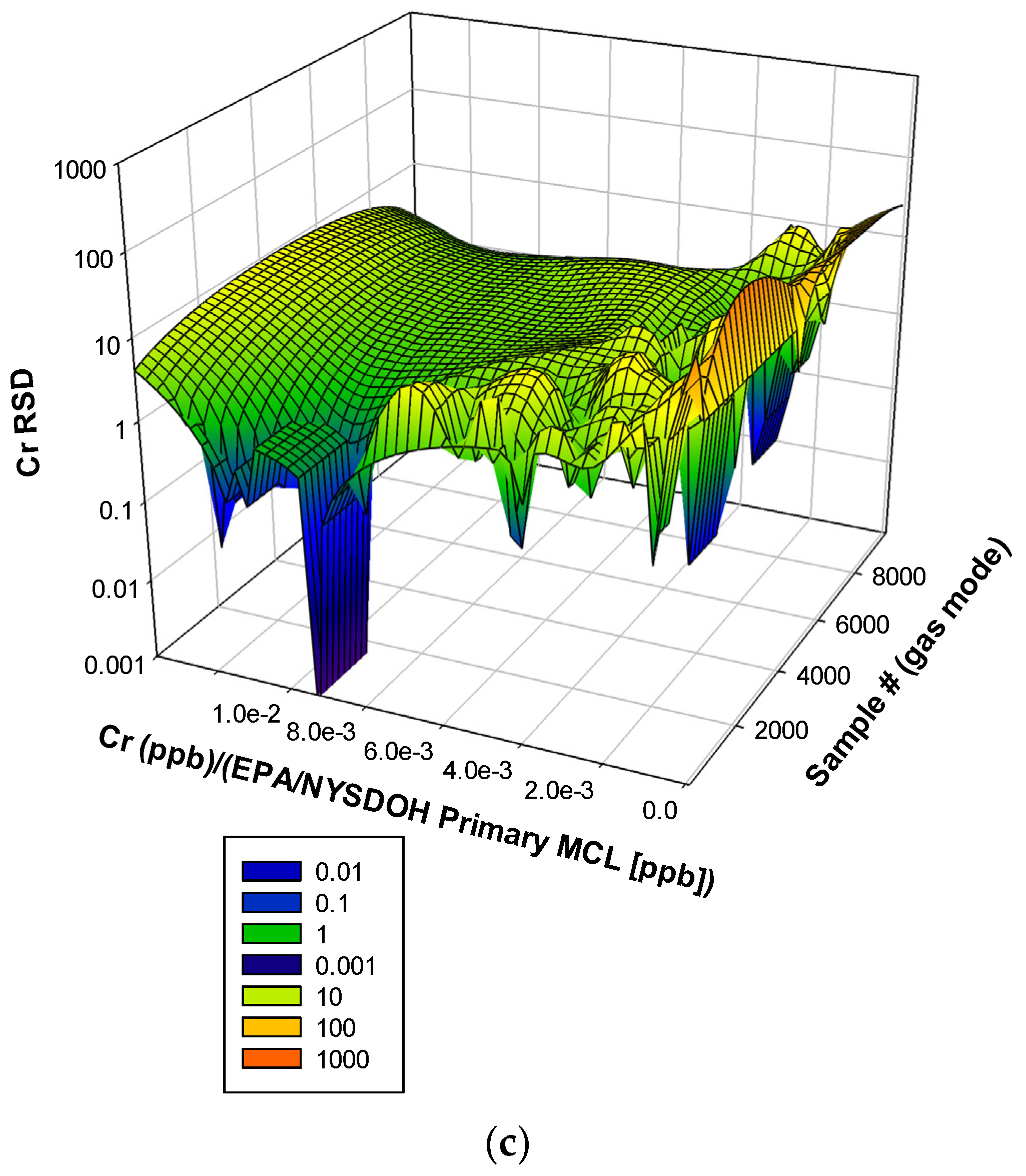
3.3. Remaining Heavy Metals
3.4. Public Health Implications toward Cancer Attainment
4. Conclusions
Supplementary Materials
Author Contributions
Funding
Data Availability Statement
Conflicts of Interest
References
- World Health Organization. Guidelines for Drinking-Water Quality, 4th ed.; Incorporating the First Addendum; World Health Organization: Geneva, Switzerland, 2017.
- World Health Organization. Guidelines for Drinking-Water Quality, 4th ed.; Incorporating the First and Second Addenda; World Health Organization: Geneva, Switzerland, 2022.
- Cotruvo, J.; Craun, G.; Nancy Hearne, N. Providing Safe Drinking Water in Small Systems: Technology, Operations, and Economics; CRC Press: Boca Raton, FL, USA, 2019. [Google Scholar]
- Jain, R. Providing safe drinking water: A challenge for humanity. Clean Technol. Environ. Policy 2012, 14, 1–4. [Google Scholar] [CrossRef]
- Ahuja, A.; Kremer, M.; Zwane, A.P. Providing Safe Water: Evidence from Randomized Evaluations. Annu. Rev. Resour. Econ. 2010, 2, 237–256. [Google Scholar] [CrossRef]
- Weinmeyer, R.; Norling, A.; Kawarski, M.; Higgins, E. The Safe Drinking Water Act of 1974 and Its Role in Providing Access to Safe Drinking Water in the United States. AMA J. Ethics 2017, 19, 1018–1026. [Google Scholar] [CrossRef]
- Fuller, R.; Landrigan, P.J.; Balakrishnan, K.; Bathan, G.; Bose-O’Reill, S.; Brauer, M.; Caravanos, J.; Chiles, T.; Cohen, A.; Corra, L.; et al. Pollution and health: A progress update. Lancet 2022, 6, E535–E547. [Google Scholar] [CrossRef] [PubMed]
- Gadgil, A.J.; Derby, E.A. Providing Safe Drinking Water to 1.2 Billion Unserved People. 2003. Available online: https://www.osti.gov/biblio/815500 (accessed on 11 October 2023).
- Hudrey, S.E.; Hudrey, E.J. Safe Drinking Water; IWA Publishing: London, UK, 2004. [Google Scholar]
- Hudrey, S.; Hudrey, E.; Pollard, S. Risk management for assuring safe drinking water. Environ. Int. 2016, 32, 948–957. [Google Scholar] [CrossRef]
- Medema, G.J.; Payment, P.; Dufour, A.; Robertson, W.; Waite, M.; Kirby, R.; Anderson, Y. Assessing Microbial Safety of Drinking Water: Improving Approaches and Methods; World Health Organization: Geneva, Switzerland, 2003.
- Ruckart, P.Z.; Ettinger, A.S.; Hanna-Attisha, M.; Jones, N.; Davis, S.I.; Breysse, P.N. The Flint Water Crisis: A Coordinated Public Health Emergency Response and Recovery Initiative. J. Public Health Manag. Pract. 2019, 25 (Suppl. S1), S84–S90. [Google Scholar] [CrossRef]
- Hanna-Attisha, M. What the Eyes Don’t See—A Story of Crisis, Resistance, and Hope in an American City; Random House Publishing Group: New York, NY, USA, 2019. [Google Scholar]
- Zheng, S.; LeWinn, K.; Ceja, T.; Hanna-Attisha, M.; O’Connell, L.; Bishop, S. Adaptive Behavior as an Alternative Outcome to Intelligence Quotient in Studies of Children at Risk: A Study of Preschool-Aged Children in Flint, MI, USA. Front. Psychol. 2021, 12, 692330. [Google Scholar] [CrossRef] [PubMed]
- Zheng, S.; Bishop, S.L.; Ceja, T.; Hanna-Attisha, M.; LeWinn, K. Neurodevelopmental profiles of preschool-age children in Flint, Michigan: A latent profile analysis. J. Neurodev. Disord 2021, 13, 29. [Google Scholar] [CrossRef] [PubMed]
- Kolowich, S. The Water Next Time: Professor Who Helped Expose Crisis in Flint Says Public Science Is Broken; The Chronicle of Higher Education: Washington, DC, USA, 2016; Available online: https://www.davidrasnick.com/ewExternalFiles/Kolowich%202016%20Public%20Science%20Is%20Broken.pdf (accessed on 15 May 2023).
- Egan, P. President Obama Declares Emergency in Flint; Ex-EPA Official Defends Agency’s Work in Flint Water Crisis at Capitol Hill Hearing Archived 2016-03-19 at the Wayback Machine MSN, March 15, 2016; Former EM Removed from Witness List for Congressional Hearing on Flint Water the Flint Journal via MLive, February 2, 2016. Available online: https://obamawhitehouse.archives.gov/the-press-office/2016/05/03/fact-sheet-federal-support-flint-water-crisis-response-and-recovery (accessed on 11 October 2023).
- Chris, D. How a Stubborn Pediatrician Forced the State to Take Flint’s Water Crisis Seriously. Available online: https://www.huffpost.com/entry/pediatrician-forced-state-to-take-flint-crisis-seriously_n_569febbfe4b076aadcc5014e (accessed on 29 July 2022).
- Itkowitz, C. The Heroic Professor Who Helped Uncover the Flint Lead Water Crisis Has Been Asked to Fix It. Washington Post, 26 January 2016. [Google Scholar]
- Ron Fonger, Gov. Snyder Signs Executive Order to Create New Flint Water Committee, The Flint Journal via MLive (11 January 2016). Available online: https://www.michigan.gov/-/media/Project/Websites/formergovernors/Folder6/FWATF_FINAL_REPORT_21March2016.pdf?rev=284b9e42c7c840019109eb73aaeedb68 (accessed on 17 August 2023).
- Adams and Aggarwala New York City Drinking Water Supply and Quality Report 2022. Available online: https://www.nyc.gov/assets/dep/downloads/pdf/water/drinking-water/drinking-water-supply-quality-report/2022-drinking-water-supply-quality-report.pdf (accessed on 27 April 2023).
- Eaton; Andrew, D.; Franson, M.A.H. Standard Methods for Examining Water and Wastewater; American Public Health Association: Washington, DC, USA; American Water Works Association: Denver, CO, USA; Water Environment Federation: Alexandria, VA, USA, 2005. [Google Scholar]
- Chowdhury, S.; Mazunder, M.A.J.; Al-Attas, O.; Husain, T. Heavy metals in drinking water: Occurrences, implications, and future needs in developing countries. Sci. Total Environ. 2016, 569–570, 476–488. [Google Scholar] [CrossRef]
- Levin, R.; Schock, M.R.; Marcus, A.H. Exposure to lead in U.S. drinking water. In Proceedings of the 23rd Annual Conference on Trace Substances in Environmental Health, Cincinnati, OH, USA, 8–12 July 1990; US Environmental Protection Agency: Washington, DC, USA, 1989. [Google Scholar]
- Schock, M.R. Understanding lead corrosion control strategies. J. Am. Water Work. Assoc. 1989, 81, 88. [Google Scholar] [CrossRef]
- Schock, M.R. Causes of temporal variability of lead in domestic plumbing systems. Environ. Monit. Assess. 1990, 15, 59. [Google Scholar] [CrossRef]
- Cosgrove, E.; Brown, M.J.; Madigan, P.; McNulty, P.; Okonski, L.; Schmidt, J. Childhood lead poisoning: Case study traces source to drinking water. J. Environ. Health 1989, 52, 346. [Google Scholar]
- Moore, M.R.; Goldberg, A.; Fyfe, W.M.; Richards, W.N. Maternal lead levels after alterations to water supply. Lancet 1981, 2, 203–204. [Google Scholar] [CrossRef] [PubMed]
- Sherlock, J.C.; Quinn, M.J. Relationship between blood lead concentrations and dietary lead intake in infants: The Glasgow Duplicate Diet Study 1979–1980. Food Addit. Contam. 1986, 3, 167–176. [Google Scholar] [CrossRef] [PubMed]
- Dabeka, R.W.; McKenzie, A.D.; Lacroix, G.M.A. Dietary intakes of lead, cadmium, arsenic and fluoride by Canadian adults: A 24-hour duplicate diet study. Food Addit. Contam. 1987, 4, 89–101. [Google Scholar] [CrossRef]
- Department of National Health and Welfare (Canada). Guidelines for Canadian Drinking Water Quality: Supporting Documentation; Department of National Health and Welfare: Ottawa, ON, Canada, 1992. [Google Scholar]
- Quinn, M.J.; Sherlock, J.C. The correspondence between U.K. ‘action levels’ for lead in blood and in water. Food Addit. Contam. 1990, 7, 387–424. [Google Scholar] [CrossRef]
- Galal-Gorchev, H. Dietary intake of pesticide residues, cadmium, mercury and lead. Food Addit. Contam. 1991, 8, 793–806. [Google Scholar] [CrossRef] [PubMed]
- US Environmental Protection Agency. Air Quality Criteria for Lead; Report EPA-600/8-83/028F; US Environmental Protection Agency: Research Triangle Park, NC, USA, 1986.
- Drill, S.; Konz, J.; Mahar, R.; Morse, M. The Environmental Lead Problem: An Assessment of Lead in Drinking Water from a Multi-Media Perspective; Report EPA-570/9-79-003; US Environmental Protection Agency: Washington, DC, USA, 1979.
- Clausing, P.; Brunekreef, B.; van Wijnen, J.H. A method for estimating soil ingestion by children. Int. Arch. Occup. Environ. Health 1987, 59, 73–82. [Google Scholar] [CrossRef] [PubMed]
- Van Wijnen, J.H.; Clausing, P.; Brunekreef, B. Estimated soil ingestion by children. Environ. Res. 1990, 51, 147–162. [Google Scholar] [CrossRef]
- Campbell, B.C.; Baird, A.W. Lead poisoning in a group of demolition workers. Occupational Environ. Med. 1977, 34, 298–304. [Google Scholar] [CrossRef]
- Ritz, E.; Mann, J.; Wiecek, A. Does lead play a role in the development of renal insufficiency? Contrib. Nephrol. 1988, 64, 43–48. [Google Scholar]
- Pocock, S.J.; Shaper, A.G.; Ashby, D.; Delves, T.; Whitehead, T.P. Blood lead concentration, blood pressure, and renal function. Br. Med. J. 1984, 289, 872–874. [Google Scholar] [CrossRef]
- Harlan, W.R.; Landis, J.R.; Schmouder, R.L.; Goldstein, N.G.; Harlan, L.C. Blood lead and blood pressure. Relationship in the adolescent and adult US population. J. Am. Med. Assoc. 1985, 253, 530–534. [Google Scholar] [CrossRef]
- Gartside, P.S. Re: “The relationship between blood lead levels and blood pressure and its cardiovascular risk implications”. Am. J. Epidemiol. 1986, 124, 864–867. [Google Scholar] [CrossRef] [PubMed]
- Moore, M.R. Haematological effects of lead. Sci. Total Environ. 1988, 71, 419–431. [Google Scholar] [CrossRef] [PubMed]
- Joint FAO/WHO Expert Committee on Food Additives. In Toxicological Evaluation of Certain Food Additives and Contaminants; WHO Food Additives Series, No. 21; Cambridge University Press: Cambridge, UK, 1987; pp. 223–255.
- Granick, J.L.; Sassa, S.; Granick, S.; Levere, R.D.; Kappas, A. Studies in lead poisoning. II. Correlation between the ratio of activated to inactivated delta-aminolevulinic acid dehydratase of whole blood and the blood lead level. Biochem. Med. 1973, 8, 149–159. [Google Scholar] [CrossRef] [PubMed]
- Mushak, P.; Davis, J.M.; Crocetti, A.F.; Grant, L.D. Prenatal and postnatal effects of low-level lead exposure: Integrated summary of a report to the US Congress on childhood lead poisoning. Environ. Res. 1989, 50, 11–36. [Google Scholar] [CrossRef] [PubMed]
- Piomelli, S.; Seaman, C.; Zullow, D.; Curran, A.; Davidow, B. Threshold for lead damage to heme synthesis in urban children. Proc. Natl. Acad. Sci. USA 1982, 79, 3335–3339. [Google Scholar] [CrossRef]
- Roels, H.A.; Bruaux, P.; Buchet, J.P.; Claeys-Thoreau, F.; Lauwerys, R.; Lafontaine, A.; Hubermont, G.; Van Overschelde, J. Impact of air pollution by lead on the heme biosynthetic pathway in school-age children. Arch. Environ. Health 1976, 31, 310–316. [Google Scholar] [CrossRef]
- Rabinowitz, M.B.; Leviton, A.; Needleman, H.L. Occurrence of elevated protoporphyrin levels in relation to lead burden in infants. Environ. Res. 1986, 39, 253–257. [Google Scholar] [CrossRef]
- Grandjean, P.; Lintrup, J. Erythrocyte-Zn-protoporphyrin as an indicator of lead exposure. Scand. J. Clin. Lab. Investig. 1978, 38, 669–675. [Google Scholar] [CrossRef] [PubMed]
- Toriumi, H.; Kawai, M. Free erythrocyte protoporphyrin (FEP) in a general population, workers exposed to low-level lead, and organic-solvent workers. Environ. Res. 1981, 25, 310–316. [Google Scholar] [CrossRef] [PubMed]
- Angle, C.R.; Kuntzelman, D.R. Increased erythrocyte protoporphyrins and blood lead—A pilot study of childhood growth patterns. J. Toxicol. Environ. Health 1989, 26, 149–156. [Google Scholar] [CrossRef] [PubMed]
- Schwartz, J.; Angle, C.; Pitcher, H. Relationship between childhood blood lead levels and stature. Pediatrics 1986, 77, 281–288. [Google Scholar] [CrossRef] [PubMed]
- Rosen, J.F.; Chesney, R.W.; Hamstra, A.; DeLuca, H.F.; Mahaffey, K.R. Reduction in 1,25-dihydroxyvitamin D in children with increased lead absorption. N. Engl. J. Med. 1980, 302, 1128–1131. [Google Scholar] [CrossRef]
- Lester, M.L.; Horst, R.L.; Thatcher, R.W. Protective effects of zinc and calcium against heavy metal impairment of children’s cognitive function. Nutr. Behav. 1986, 3, 145. [Google Scholar]
- Markovac, J.; Goldstein, G.W. Picomolar concentrations of lead stimulate brain protein kinase C. Nature 1988, 334, 71–73. [Google Scholar] [CrossRef]
- Otto, D.A.; Benignus, V.A.; Muller, K.E.; Barton, C.N. Effects of age and body lead burden on CNS function in young children. I. Slow Cortical Potentials. Electroencephalogr. Clin. Neurophysiol. 1981, 52, 229–239. [Google Scholar] [CrossRef]
- Otto, D.A.; Benignus, V.; Muller, K.; Barton, C.; Seiple, K.; Prah, J.; Schroeder, S. Effects of low to moderate lead exposure on slow cortical potentials in young children: Two-year follow-up study. Neurobehav. Toxicol. Teratol. 1982, 4, 733–737. [Google Scholar]
- Schwartz, J.; Landrigan, P.J.; Feldman, R.G.; Silbergeld, E.K.; Baker, E.L., Jr.; von Lindern, I.H. Threshold effect in lead-induced peripheral neuropathy. J. Pediatr. 1988, 112, 12–17. [Google Scholar] [CrossRef]
- Robinson, G.S.; Morata, T.C.; Lopes, A.C.; Feniman, M.R.; Corteletti, L.C. Effects of low to moderate lead exposure on brainstem auditory evoked potentials in children. In Neurobehavioural Methods in Occupational and Environmental Health; Environmental Health Series No. 3; WHO Regional Office for Europe: Copenhagen, Denmark, 1985; p. 177. [Google Scholar]
- Schwartz, J.; Otto, D. Blood lead, hearing thresholds, and neurobehavioral development in children and youth. Arch. Environ. Health 1987, 42, 153–160. [Google Scholar] [CrossRef]
- Lancranjan, I. Reproductive ability of workmen occupationally exposed to lead. Arch. Environ. Health 1975, 30, 396–401. [Google Scholar] [CrossRef] [PubMed]
- Wildt, K.; Eliasson, R.; Berlin, M. Effects of occupational exposure to lead on sperm and semen. In Reproductive and Developmental Toxicity of Metals; Plenum Press: Rochester, NY, USA, 1983; pp. 279–300. [Google Scholar]
- Cullen, M.R.; Kayne, R.D.; Robins, J.M. Endocrine and reproductive dysfunction in men associated with occupational inorganic lead intoxication. Arch. Environ. Health 1984, 39, 431–440. [Google Scholar] [CrossRef]
- Assennato, G.; Paci, C.; Baser, M.E.; Molinini, R.; Candela, R.G.; Altamura, B.M.; Giorgino, R. Sperm count suppression without endocrine dysfunction in lead-exposed men. Arch. Environ. Health 1986, 4, 387–390. [Google Scholar] [CrossRef] [PubMed]
- International Agency for Research on Cancer. Some metals and metallic compounds. In IARC Monographs on the Evaluation of Carcinogenic Risks to Humans; International Agency for Research on Cancer: Lyon, France, 1980; Volume 23, p. 325. [Google Scholar]
- McMichael, A.J.; Vimpani, G.V.; Robertson, E.F.; Baghurst, P.A.; Clark, P.D. The Port Pirie cohort study: Maternal blood lead and pregnancy outcome. J. Epidemiol. Community Health 1986, 40, 18–25. [Google Scholar] [CrossRef] [PubMed]
- Needleman, H.; Rabinowitz, M.; Leviton, A.; Linn, S.; Schoenbaum, S. The relationship between prenatal lead exposure and congenital anomalies. J. Am. Med. Assoc. 1984, 251, 2956–2959. [Google Scholar] [CrossRef]
- International Agency for Research on Cancer. Overall evaluations of carcinogenicity: An updating of IARC monographs volumes 1–42. In IARC Monographs on the Evaluation of Carcinogenic Risks to Humans, Suppl. 7; International Agency for Research on Cancer: Lyon, France, 1987; pp. 230–232. [Google Scholar]
- Cooper, W.C.; Gaffey, W.R. Mortality of lead workers. J. Occup. Med. 1975, 17, 100–107. [Google Scholar] [CrossRef] [PubMed]
- Kang, H.K.; Infante, P.R.; Carra, J.S. Occupational lead exposure and cancer. Science 1980, 20, 935–936. [Google Scholar] [CrossRef]
- Cooper, W.C.; Wong, O.; Kheifets, L. Mortality among employees of lead battery plants and lead producing plants, 1947–1980. Scand. J. Work. Environ. Health 1985, 11, 331–345. [Google Scholar] [CrossRef]
- McMichael, A.J.; Johnson, H.M. Long-term mortality profile of heavily-exposed lead smelter workers. J. Occup. Med. 1982, 24, 375–378. [Google Scholar] [CrossRef]
- Smith, M. The effects of low-level lead exposure on children. In Lead Exposure and Child Development: An International Assessment; Smith, M.A., Grant, L.D., Sors, A.I., Eds.; Kluwer Academic Publishers: Boston, MA, USA, 1989; p. 3. [Google Scholar]


Disclaimer/Publisher’s Note: The statements, opinions and data contained in all publications are solely those of the individual author(s) and contributor(s) and not of MDPI and/or the editor(s). MDPI and/or the editor(s) disclaim responsibility for any injury to people or property resulting from any ideas, methods, instructions or products referred to in the content. |
© 2023 by the authors. Licensee MDPI, Basel, Switzerland. This article is an open access article distributed under the terms and conditions of the Creative Commons Attribution (CC BY) license (https://creativecommons.org/licenses/by/4.0/).
Share and Cite
Blaszczak-Boxe, C.S.; Karle, N.N.; Wang, S.; Yu, M.; Golosov, N.; Riyad, M.; Smith, K.; Hollet, T.; Abdul-Hamid, B.; St. Hillaire, D.; et al. Environmental Assessment and Monitoring of Heavy Metals in New York City Potable Water Systems: Case Study at Medgar Evers College, Correlation Analysis, and Public Health Impacts. Water 2023, 15, 4233. https://doi.org/10.3390/w15244233
Blaszczak-Boxe CS, Karle NN, Wang S, Yu M, Golosov N, Riyad M, Smith K, Hollet T, Abdul-Hamid B, St. Hillaire D, et al. Environmental Assessment and Monitoring of Heavy Metals in New York City Potable Water Systems: Case Study at Medgar Evers College, Correlation Analysis, and Public Health Impacts. Water. 2023; 15(24):4233. https://doi.org/10.3390/w15244233
Chicago/Turabian StyleBlaszczak-Boxe, Christopher S., Nakul N. Karle, Shujie Wang, Manzhu Yu, Nikolay Golosov, Mohammed Riyad, Kayla Smith, Ty Hollet, Bishara Abdul-Hamid, Dickens St. Hillaire, and et al. 2023. "Environmental Assessment and Monitoring of Heavy Metals in New York City Potable Water Systems: Case Study at Medgar Evers College, Correlation Analysis, and Public Health Impacts" Water 15, no. 24: 4233. https://doi.org/10.3390/w15244233
APA StyleBlaszczak-Boxe, C. S., Karle, N. N., Wang, S., Yu, M., Golosov, N., Riyad, M., Smith, K., Hollet, T., Abdul-Hamid, B., St. Hillaire, D., & Sen, P. (2023). Environmental Assessment and Monitoring of Heavy Metals in New York City Potable Water Systems: Case Study at Medgar Evers College, Correlation Analysis, and Public Health Impacts. Water, 15(24), 4233. https://doi.org/10.3390/w15244233